Assessing Intra-Row Spacing Using Image Processing: A Promising Digital Tool for Smallholder Farmers

Abstract

Assessing planting to ensure well-distributed plants is important to achieve high yields. Digital farming has been helpful in these field assessments. However, these techniques are at most times not available for smallholder farmers or low-income regions. Thus, to contribute such producers, we developed two methods to assess intra-row spacing in commercial fields using mobile photos and simple image processing. We assessed a maize field after mechanized planting in 7 and 12 days after planting (DAP) and in two farming systems (conventional and no-till) to acquire images at height of one meter and perpendicular to the ground. In the first method, we used morphological operations based on the HSV scale and the center of mass to extract the region of interest (ROI) corresponding to the maize plant. In the second method, we used local maxima equations (Peaks) to find prominence values corresponding to the maize plant and extract their coordinates. No-till images were deleted due to excessive weeds. Thus, before acquiring the images, it is necessary to remove these elements (e.g., no-till adapted). The methods achieved an overall RMSE of 3.48 cm (<5.63 cm) and R² of 0.90 (>0.71) between the actual and estimated spacing. Precision and recall were higher than 0.88. There was no difference between actual and estimated CV values, except in conventional tillage in 7 DAP using ROI due to leaves overlapping. The method Peaks was more accurate to detect multiple spacing but miss spacing was correctly detected in both methods. However, the larger the plant leaves, the worse the detection. Thus, our proposed methods were satisfactory and are promising for assessing planting in a remote and accessible way.

1. Introduction

Well-distributed seeds support plant development by reducing nutrient competition against weeds [1]. Moreover, it can adjust the population density and contribute to yield gains [2]. For every 10 percentage points added in the coefficient of variation of intra-row spacing, about 1.22 Mg ha⁻¹ of maize grain would not be yielded in some fields [3]. Thus, the spacing between plants should be as equidistant as possible, with high uniformity. Another assessment refers to machine performance. Seed or emerged plant distribution in any crop can demonstrate the machine efficiency to deposit seeds along the crop row [4]. However, seeds are below-ground and invisible to the machine operator, and no real-time resources are available for on-field measurements, only for laboratory conditions [5,6]. Seed spacing can be assessed by digging and counting, but plant spacing is available only after emergence. If, however, the intra-row has much miss-spacing, it may indicate low-vigor seeds or a poorly adjusted machine. Multiple spacing or multiple plants together also indicates poor adjustment. The farmer should adjust the machine for the next area or season based on these results.

The traditional assessment of plant distribution consists of measurements using tape measure or any standard tool. However, it can be laborious and time-consuming since most field methods are based on manual techniques suggested decades ago when few technologies were available [7]. Several digital tools have been developed to replace these manual and labor-intensive methods. By way of example, computer vision and remote sensing have become key tools [8]. The development of these versatile tools is encouraged due to massive data flow in agriculture, demanding smart systems to generate knowledge. Such systems support decision-making and automate routine tasks [9]. Despite a digital revolution in agriculture, few tools exist to assess intra-row spacing in commercial fields. An often alternative from the regular literature for assessing intra-row spacing is using ultrasonic sensors, 3D scanners or LiDAR embedded in mobile structures to detect objects by point cloud or the time of the flight principle (TOF) [10,11,12]. The method by Nakarmi and Tang [12] relies on a system that collects TOF images in crop inter-row to find the stem of each plant and measure the spacing. It produces a R² up to 0.95 and RMSE up to 0.017 cm. Few researchers have assessed the intra-row spacing using only imaging techniques. A ground vehicle with an embedded camera can be used to acquire images. Then, the maize plants are detected using Naïve Bayes, and following post-processing, the intra-row spacing can be measured [13]. In a similar study, Brilhador et al. [14] used morphological operations and a vegetation index (generated by RGB colors) to detect maize plants. They found precision results ranging from 59% (with straw and mature plants) to 89% for plant stems. For intra-row spacing, error up to 1 cm was described; however, no further testing was performed with these data. Studies also quantified plant population density. Liu et al. [15] used a mobile structure to take images of a wheat crop. They manually determined for each image the coordinates of each existent plant. It produces a relative error up to 12% in relation to actual population density. A successfully emerging method is remote sensing using an unnamed aerial vehicle (UAV) embedded with RGB or multispectral cameras. Machine learning models can detect plants in these high-resolution images that provide useful and versatile data to analyze plantation arrangement [16,17].

However, high-complexity methods and expensive equipment do not necessarily help farmers, especially the small ones. Digital agriculture is described in some countries as a well-known benefic system but few farmers can support these investments [18]. In contrast, new techniques such as digital maps, remote sensing, and auto-guidance are mostly available and benefit big farms that support high financial costs [19]. Digital agriculture should consider the socio-economic context of developing countries. Despite the difficult access, the use of mobile phones has spread quickly in low-income regions as some sub-Saharan countries, in contrast to the internet or more recent equipment [19]. New technologies are not sustainable without a positive social impact. The well-known justification of producing more food due to population growth is questionable since the main problem of food security is the access and inequality [20,21], which may also involve the use and availability of technologies. The regular literature Pfocuses on plant detection or counting. Thus, indispensable reasons are ignored: planting machine performance and intra-row spatial arrangement. Analysis as miss spacing, multiple spacing, and the coefficient of variation are extremely useful [7]. In addition, these metrics demand an in-depth investigation considering different tillage systems. Moreover, it is not clear how and if these techniques will serve as a basis for future digital tools, especially to the smallholders and low-income regions. Therefore, based on the need to contribute to the planting assessment with alternative, remote and accessible methods, we developed two image processing methods to assess intra-row plant spacing using mobile images.

2. Materials and Methods

2.1. Experiment Location

We conducted our study in a commercial field localized in the municipality of Cândido Mota, in the state of São Paulo, Brazil. The maize crop was planted using two farming systems: conventional tillage and no-till. The farmer adopted a population density of 70.000 plants ha⁻¹ and 3.5 seed m⁻¹ in an inter-row spacing of 50 cm.

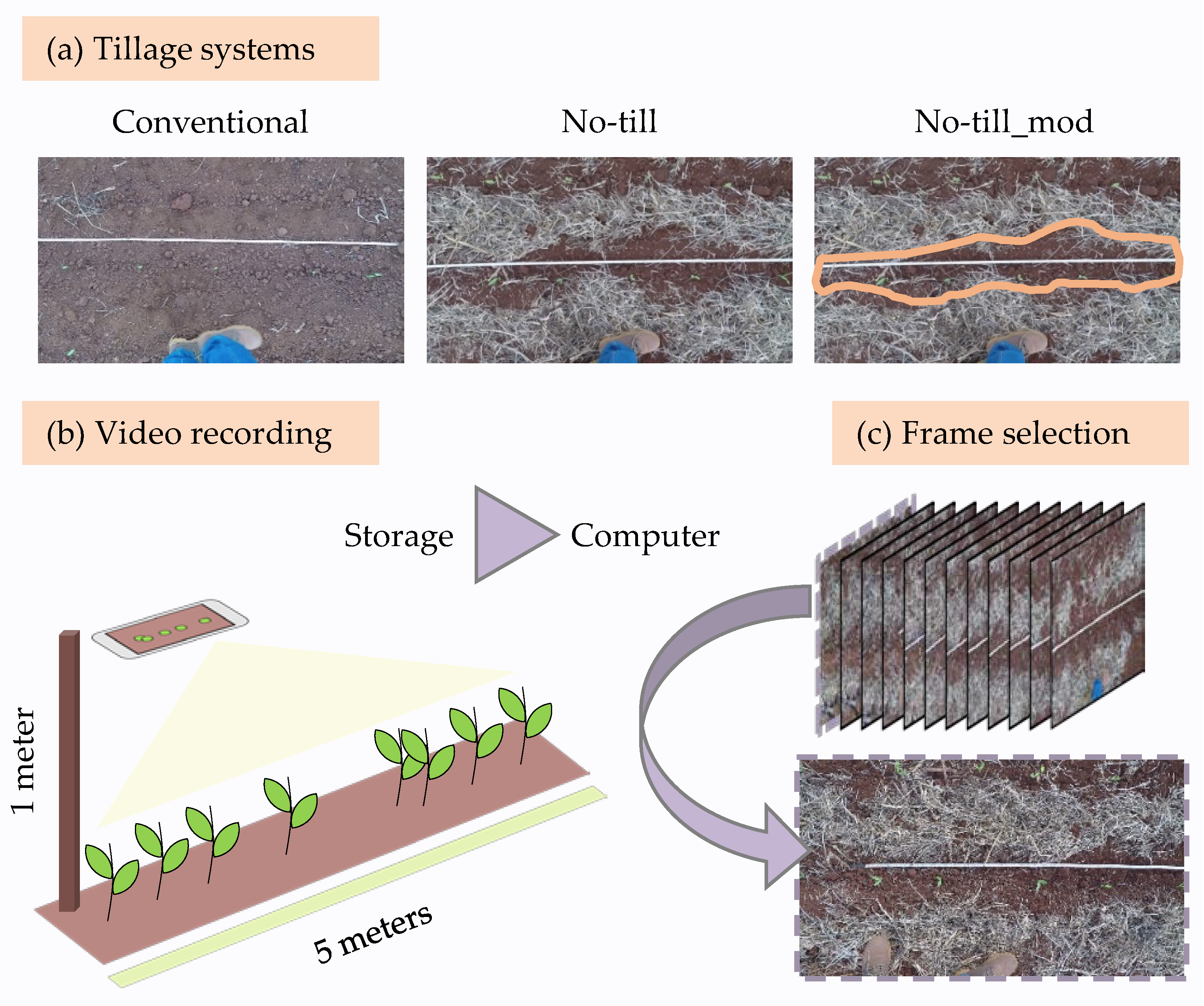
2.2. Data Collection

To capture early crop growth dynamics, data was collected in two periods: 7 and 12 days after planting (DAP). We assessed a crop row in both tillage systems to count each plant and measure the intra-row spacing across five meters. To facilitate image acquisition, we recorded a video using a mobile camera with resolutions of 13 MP, 1080 P, and 30 FPS (Figure 1b). To ensure an adequate pixel spatial resolution and minimal distortions [15], a height of one meter and a perpendicular angle (90°) were considered as the reference. We used a level indicator from the mobile device to maintain its stability and a standardized object beside the crop row. To avoid differences over day lighting, we recorded every video at the same hour: about 04:00 pm in clear sky. No-till rows were recorded twice: with an original aspect and after cleaning excessive organic material, weeds or plants remain from the harvesting, which may affect the image processing [22]. We partitioned the dataset (Figure 1a) into conventional (Conv_), no-till (Notill_), and no-till after cleaning (Notill_mod). The images were extracted from each video (Figure 1c). We selected images based on perpendicularity, blurring, and motion.

2.3. Image Processing

We processed the images using the OpenCV [23] and scikit-image [24] libraries in a pipeline developed in Python (code available upon request). Our main goal was to extract features (green objects) and measure the spacing between them in a semi-automatic way. We used two methods: in the first, we detected the region of interest (ROI) and created bounding boxes; in the second, we used a gray-scale histogram to detect peaks values that correspond to maize plants (Figure 2).

2.3.1. Pre-Processing

To standardize the input image, each one was cropped to remove parallel rows and a Gaussian filter was used in 3 × 3 sizes to reduce pixel noises. The next step was to determine the spectrum corresponding to the green in a HSV scale and highlight only green objects. At the same time, we applied a slight dilatation to smooth the noise around the plant and emphasize the ROI mainly due to leaf twisting or points of dim illumination.

2.3.2. Region of Interest (ROI)

In the first method, we created boxes around the binary objects (maize plants) using the boundingRect function. The coordinates of these bounding boxes were extracted and we calculated the center of mass (Figure 2) using the ‘moments calculus’, which considers pixels’ distribution in a given area to determine the center [25], as described in Equation (1):

$${\mathrm{M}}_{00}={\displaystyle \sum }_x{\displaystyle \sum }_{y}l(x,y)$$

(1)

where M₀₀ is the moment zero and x and y are the pixel values in each contour in the bounding box. The following replacements were made at the positions to calculate the first moment on each axis (x, y), according to Equation (2):

$${\mathrm{M}}_{10}={\displaystyle \sum }_x{\displaystyle \sum }_y\mathit{xl}(x,y); {\mathrm{M}}_{01}={\displaystyle \sum }_x{\displaystyle \sum }_y\mathit{yl}(x,y)$$

(2)

Finally, the center of mass coordinates can be calculated using Equation (3):

$$\mathit{xc}=\frac{{\mathrm{M}}_{10}}{{\mathrm{M}}_{00}}; \mathit{yc}=\frac{{\mathrm{M}}_{01}}{{\mathrm{M}}_{00}}$$

(3)

2.3.3. Local Maxima (Peaks)

In the second method, our approach was based on finding pixel gray-scale values corresponding to the plant. A peak is a prominent value in comparison to neighboring pixels. A similar method was used to count crop rows and plants, extracting peaks value based on a confidence map [17]. In this way, we used the mask with plants (pre-processing) and the “peak_local_max” function from the library scikit-image. The general concept is that a function f(x) has local maxima at c if there is an open interval in I containing c so that f(x) ≤ f(c) for all values of x in I. We determined 50 pixels between peaks to avoid multiple peaks in very short distances.

2.4. Analysis

We analyzed both proposed methods using “Precision” as the chance to find a plant and “Recall” as the chance to finding any object, including plants, according to Equations (4) and (5) [26]:

$$\mathrm{Precision}=\frac{Tp}{Tp+Fp}$$

(4)

$$\mathrm{Recall}=\frac{Tp}{Tp+Fn}$$

(5)

where Tp is the number of detected plants; Fp is the number of misdetections; and Fn is the number of failed detections. The distance between centroids was calculated using the Euclidean distance (Equation (6). We converted the number of pixels to the metric system using the standardized object besides the crop row. The coefficient of determination and (R²) and Root Mean Square Error (RMSE) were used to evaluate the intra-row spacing accuracy.

$$\mathrm{d}=\sqrt{{\left(x_1-x_2\right)}^2+{\left(y_1-y_2\right)}^2}$$

(6)

where x and y indicate the plant coordinates. Specific metrics are useful for planting assessment. These values can indicate problems related to the planting or plant emergence. Therefore, we used the ‘multiple index’, which considers a multiple spacing between plants when the distance is less than or equal to half of the ideal distance, and the ‘miss index’, which considers a miss spacing when the distance is 1.5 times greater than both the ideal distance [7] and the coefficient of variation (CV). For CV, we used the Forkman test to compare significant differences (p > 0.05) [27].

3. Results

In this section we describe the overall aspects and performance (Section 3.1), and the specific assessment for planting performance (Section 3.2).

3.1. Overall Aspects and Performance

In both methods, precision and recall were above 0.88. Recall was lower in 12 DAP and using the ROI method, as the closest intra-row spacing supports the leaves overlapping and merges the two bounding boxes (Figure 3a). This problem occurs mostly as the plant grows, since its vegetative structure will grow with more and larger leaves. It did not occur in the Peaks methods. However, the detection can be also compromised if this spacing is very close since it will not be possible to distinguish the prominence value. The overall R² was 0.90, but for 12 DAP, Notill_mod_ROI was 0.71. The RMSE for the spacing values was also highest in 12 DAP with ~5.63 cm (

Table 1. Detection and accuracy results from both methods.

	Methods	Precision	Recall	R²	RMSE, cm
7 DAP	Conv_ROI	1.00	0.91	0.90	2.84
	Conv_Peaks	1.00	1.00	0.92	2.55
	Notill_mod_ROI	1.00	1.00	0.90	1.86
	Notill_mod_Peaks	1.00	1.00	0.98	1.75
12 DAP	Conv_ROI	1.00	0.88	0.98	5.63
	Conv_Peaks	1.00	0.93	0.98	5.05
	Notill_mod_ROI	1.00	0.91	0.71	4.70
	Notill_mod_Peaks	1.00	0.91	0.81	3.50

), as the coordinate point was not exactly in the plant center due to larger leaves increasing the bounding boxes’ size, thus changing the center of mass (Figure 3a).

The centroids were different between the two methods. Although these deviations are minimal, the greaterthe bounding box in ROI due to larger leaves, the less probable the centroid in the same coordinate at the Peaks. Figure 4 shows the overall aspect of detection.

3.2. Common Metrics in Planting Assessment

There is no significant difference between the CV (p > 0.05), except in Conv_ROI 7 DAP, due to multiple spacing misdetection (

Table 2. Descriptive statistics, specific planting metrics, and CV in all scenarios.

	Methods	As, cm	Std, cm	Multiple	Miss	CV
	Conv_field	40	13	1	0	0.33
7 DAP	Conv_ROI	42	6	0	0	0.14 *
	Conv_Peaks	38	12	1	0	0.31 ns
	Notill_mod_field	34	9	0	0	0.28
	Notill_mod_ROI	34	8	0	0	0.24 ns
	Notill_mod_Peaks	34	8	0	0	0.24 ns
12 DAP	Conv_field	31	18	4	2	0.58
	Conv_ROI	27	17	1	2	0.65 ns
	Conv_Peaks	27	16	3	2	0.60 ns
	Notill_mod_field	36	9	1	0	0.26
	Notill_mod_ROI	35	8	1	0	0.27 ns
	Notill_mod_Peaks	36	8	1	0	0.24 ns

^ns not significant (p > 0.05) and * significant (p < 0.05). Note: As, average spacing; Std, standard deviation; CV, coefficient of variation of intra-row spacing; Multiple, very short spacing; and Miss, very long spacing.

). Very short spacing between two plants contributes to the leaves overlapping in the ROI method, in contrast to the Peaks method. Both methods were accurate to detect miss spacing.

4. Discussion

Our research consisted of creating a remote method to replace manual intra-row assessment using an easy-to-access tool. Such an approach facilitates on-field assessment and can support smallholder farmers to assess their crops effortlessly. The great novelty of this research study, therefore, resides in solving such a task in a unified way using images acquired by a simple mobile phone. In addition, we can perform this task without the need of high-performance hardware, allowing producers or decision-makers who live in low-income regions to use them as well.

Weeds are a major problem in plant detection because they mostly have the same architecture and color as the crop. In our approach, it was enough to eliminate one dataset (Notill_). Tang and Tian [13] proposed a method that excluded these objects using their physical dimensions; however, it is not always appropriate since weeds vary in size. Thus, before acquiring the images, it is necessary to prepare the sample area. It does not mean that the straw (key component in no-till systems) must be removed. We only need to remove the weeds, as well as other common residues in agricultural areas such as stones and excesses of green organic matter. Therefore, our methods satisfied two distinct farming systems: conventional and no-till. It is beneficial because most works listed in the review used only conventional tillage soils, which is not representative for some regions. Conventional tillage is easy to analyze by image processing as there is no straw around the plant. In addition, distances were accurately measured since there was a standard tool with a known size. If we know the object’s actual size and the pixel size, no geographical system is necessary, only simple ratio equations. However, to ensure the consistency of these measurements, a high-resolution image is required [28], in addition to keeping the distance and angle as perpendicular as possible. Strong variations in these parameters can compromise the results obtained by the image. Our method did not use any structure equipment to fix the camera; we used only an object as a height reference and a level indicator of the mobile phone itself. Slight variations are expected as the person walked alongside the crop row which is not totally flat. Thus, it is necessary to remove blurred images before processing. This is a downside of accessible techniques.

The assessment of intra-row spacing can assist in decision-making for future crop implementation by understanding the origin of poor plant distribution. Previous studies had satisfactory results detecting plant stems and measuring intra-row spacing. Using a 3D sensor, Nakarmi and Tang [13] achieved an overall RMSE of 0.017 cm, outperforming the imaging techniques; our methods achieved 3.48 cm; and a comparable method from Tang and Tian [14] achieved an accuracy of 1.70 cm. The R² values were similar and greater than 0.90 but [13] achievedan R² of 0.95 and [14] achieved 0.96. However, the cost-effectiveness of our easy-to-access system outweighs these results. For our proposal, we were not able to exactly find the plant center. We obtained small lateral deviations, especially for the ROI method, where the leaves have heterogeneous distribution inside the bounding box. The sensitivity is greater using the Peaks method since it considers the local maxima value; however, color variations across the leaves can also affect it. Even so, our results demonstrated high values of R², precision, and recall. There is no difference in CV (except for Conv_ ROI 7 DAP). Miss spacing originated from very long distances between plants and they were also successfully detected. In contrast, multiple spacing is more complex. In the ROI, if the leaves between plants overlap, multiple plants become one. A manual intervention on the image can be done to break the overlapping; however, it would compromise the automation even more. The only action to assist the ROI method is to acquire images soon after emergence before the leaves grow. Image resolution should be as high as possible to detect the green object without much soil noise. In the Peaks method, due to the analysis by value prominence, there is a greater efficiency to detect multiple spacing. However, the recommendations for ROI are valid to avoid more deviations.

5. Conclusions

Our approach clearly demonstrated the applicability and accessibility of imaging techniques to assess planting distribution and intra-row arrangement. Required low computational resources and obtained satisfactory results. It is possible to use in either conventional or no-till systems. For planting assessment metrics, multiple spacing was difficult to detect since the closest distance between plants can induce their detection as a single object. The Peaks method achieved a better performance since it uses the value prominence. However, it is also recommended to avoid larger leaves (many days after planting) since they can overlap. For miss spacing, both methods were efficient, and for the coefficient of variation, only one condition obtained a significant difference. These methods can be used in any crop after mechanized planting, such as maize, soybean, beans, and cotton. However, crops with irregular or scattered spacing are not recommended due to leaves overlapping. These approaches can encourage different avenues for future assessment considering accessibility. Mobile phones are common tools in many countries, including developed or developing; therefore, we need to use more of them in this way. Among the possibilities, we can consider a mobile application based on our considerations or even the use from advisors, which must only take photos on-fieldand process it using the script, following our guidelines. The development of a totally automatic thresholding is also highly encouraged.

References

1. Karayel, D.; Wiesehoff, M.; Özmerzi, A.; Müller, J. Laboratory Measurement of Seed Drill Seed Spacing and Velocity of Fall of Seeds Using High-Speed Camera System. Comput. Electron. Agric. 2006, 50, 89–96. [Google Scholar] [CrossRef]
2. Zhang, Q.; Zhang, L.; Evers, J.; van der Werf, W.; Zhang, W.; Duan, L. Maize Yield and Quality in Response to Plant Density and Application of a Novel Plant Growth Regulator. Field Crops Res. 2014, 164, 82–89. [Google Scholar] [CrossRef]
3. Hörbe, T.A.N.; Amado, T.J.C.; Reimche, G.B.; Schwalbert, R.A.; Santi, A.L.; Nienow, C. Optimization of Within-Row Plant Spacing Increases Nutritional Status and Corn Yield: A Comparative Study. Agron. J. 2016, 108, 1962–1971. [Google Scholar] [CrossRef]
4. Badua, S.A.; Sharda, A.; Strasser, R.; Ciampitti, I. Ground Speed and Planter Downforce Influence on Corn Seed Spacing and Depth. Precis. Agric. 2021, 22, 1154–1170. [Google Scholar] [CrossRef]
5. Lei, X.; Hu, H.; Wu, W.; Liu, H.; Liu, L.; Yang, W.; Zhou, Z.; Ren, W. Seed Motion Characteristics and Seeding Performance of a Centralised Seed Metering System for Rapeseed Investigated by DEM Simulation and Bench Testing. Biosyst. Eng. 2021, 203, 22–33. [Google Scholar] [CrossRef]
6. Xia, L.; Wang, X.; Geng, D.; Zhang, Q. Performance Monitoring System for Precision Planter Based on MSP430-CT171. In Computer and Computing Technologies in Agriculture IV; Li, D., Liu, Y., Chen, Y., Eds.; Springer: Berlin/Heidelberg, Germany, 2011; pp. 158–165. [Google Scholar] [CrossRef] [Green Version]
7. Kachman, S.D.; Smith, J.A. Alternative Measures of Accuracy in Plant Spacing for Planters Using Single Seed Metering. Trans. ASAE 1995, 38, 379–387. [Google Scholar] [CrossRef]
8. Tian, H.; Wang, T.; Liu, Y.; Qiao, X.; Li, Y. Computer Vision Technology in Agricultural Automation—A Review. Inf. Process. Agric. 2020, 7, 1–19. [Google Scholar] [CrossRef]
9. Sparrow, R.; Howard, M. Robots in Agriculture: Prospects, Impacts, Ethics, and Policy. Precis. Agric. 2020, 22, 818–833. [Google Scholar] [CrossRef]
10. Shi, Y.; Wang, N.; Taylor, R.K.; Raun, W.R.; Hardin, J.A. Automatic Corn Plant Location and Spacing Measurement Using Laser Line-Scan Technique. Precis. Agric. 2013, 14, 478–494. [Google Scholar] [CrossRef] [Green Version]
11. Shi, Y.; Wang, N.; Taylor, R.K.; Raun, W.R. Improvement of a Ground-LiDAR-Based Corn Plant Population and Spacing Measurement System. Comput. Electron. Agric. 2015, 112, 92–101. [Google Scholar] [CrossRef]
12. Nakarmi, A.D.; Tang, L. Automatic Inter-Plant Spacing Sensing at Early Growth Stages Using a 3D Vision Sensor. Comput. Electron. Agric. 2012, 82, 23–31. [Google Scholar] [CrossRef]
13. Tang, L.; Tian, L.F. Plant Identification in Mosaicked Crop Row Images for Automatic Emerged Corn Plant Spacing Measurement. Trans. ASABE 2008, 51, 2181–2191. [Google Scholar] [CrossRef]
14. Brilhador, A.; Serrarens, D.A.; Lopes, F.M. A Computer Vision Approach for Automatic Measurement of the Inter-Plant Spacing. In Progress in Pattern Recognition, Image Analysis, Computer Vision, and Applications; Lecture Notes in Computer Science; Pardo, A., Kittler, J., Eds.; Springer International Publishing: Cham, Switzerland, 2015; pp. 219–227. [Google Scholar] [CrossRef]
15. Liu, S.; Baret, F.; Allard, D.; Jin, X.; Andrieu, B.; Burger, P.; Hemmerlé, M.; Comar, A. A Method to Estimate Plant Density and Plant Spacing Heterogeneity: Application to Wheat Crops. Plant Methods 2017, 13, 38. [Google Scholar] [CrossRef] [PubMed] [Green Version]
16. Hosseiny, B.; Rastiveis, H.; Homayouni, S. An Automated Framework for Plant Detection Based on Deep Simulated Learning from Drone Imagery. Remote Sens. 2020, 12, 3521. [Google Scholar] [CrossRef]
17. Osco, L.P.; dos Santos de Arruda, M.; Gonçalves, D.N.; Dias, A.; Batistoti, J.; de Souza, M.; Gomes, F.D.G.; Ramos, A.P.M.; de Castro Jorge, L.A.; Liesenberg, V.; et al. A CNN Approach to Simultaneously Count Plants and Detect Plantation-Rows from UAV Imagery. ISPRS J. Photogramm. Remote Sens. 2021, 174, 1–17. [Google Scholar] [CrossRef]
18. Anitei, M.; Veres, C.; Pisla, A. Research on Challenges and Prospects of Digital Agriculture. Proceedings 2021, 63, 67. [Google Scholar] [CrossRef]
19. Deichmann, U.; Goyal, A.; Mishra, D. Will Digital Technologies Transform Agriculture in Developing Countries? Agric. Econ. 2016, 47 (Suppl. S1), 21–33. [Google Scholar] [CrossRef]
20. Nally, D. Against Food Security: On Forms of Care and Fields of Violence. Glob. Soc. 2016, 30, 558–582. [Google Scholar] [CrossRef]
21. Rose, D.C.; Wheeler, R.; Winter, M.; Lobley, M.; Chivers, C.-A. Agriculture 4.0: Making It Work for People, Production, and the Planet. Land Use Policy 2021, 100, 104933. [Google Scholar] [CrossRef]
22. Hamuda, E.; Mc Ginley, B.; Glavin, M.; Jones, E. Automatic Crop Detection under Field Conditions Using the HSV Colour Space and Morphological Operations. Comput. Electron. Agric. 2017, 133, 97–107. [Google Scholar] [CrossRef]
23. Bradski, G.; Kaehler, A. Learning OpenCV: Computer Vision with the OpenCV Library; O’Reilly Media, Inc.: Newton, MA, USA, 2008. [Google Scholar]
24. van der Walt, S.; Schönberger, J.L.; Nunez-Iglesias, J.; Boulogne, F.; Warner, J.D.; Yager, N.; Gouillart, E.; Yu, T. Scikit-Image: Image Processing in Python. PeerJ 2014, 2, e453. [Google Scholar] [CrossRef] [PubMed]
25. Teh, C.-H.; Chin, R.T. On Image Analysis by the Methods of Moments. In Proceedings of the CVPR’88: The Computer Society Conference on Computer Vision and Pattern Recognition, Ann Arbor, MI, USA, 5–9 June 1988; IEEE Computer Society Press: Ann Arbor, MI, USA, 1988; pp. 556–561. [Google Scholar] [CrossRef]
26. Lu, H.; Cao, Z.; Xiao, Y.; Fang, Z.; Zhu, Y.; Xian, K. Fine-Grained Maize Tassel Trait Characterization with Multi-View Representations. Comput. Electron. Agric. 2015, 118, 143–158. [Google Scholar] [CrossRef]
27. Forkman, J. Estimator and Tests for Common Coefficients of Variation in Normal Distributions. Commun. Stat. Theory Methods 2009, 38, 233–251. [Google Scholar] [CrossRef] [Green Version]
28. Jin, X.; Liu, S.; Baret, F.; Hemerlé, M.; Comar, A. Estimates of Plant Density of Wheat Crops at Emergence from Very Low Altitude UAV Imagery. Remote Sens. Environ. 2017, 198, 105–114. [Google Scholar] [CrossRef] [Green Version]
Figure 1. (a) Tillage systems used to create our dataset; (b) video recording technique and (c) manual frame selection.
Agronomy 12 00301 g001
Figure 2. Organized dataset and morphological operations using Python libraries.
Agronomy 12 00301 g002
Figure 3. Illustrative example of (a) misdetection due to leaves overlapping and (b) intra-row weeds.
Agronomy 12 00301 g003
Figure 4. Overall aspect from both methods (no-till adapted).
Agronomy 12 00301 g004