Is It Possible to Assess Heatwave Impact on Grapevines at the Regional Level with Time Series of Satellite Images?

Abstract

Unexpected climatic conditions or extreme climatic events in vineyards are a worldwide problem that requires accurate spatial and temporal monitoring. Satellite-based remote sensing is an important source of data to assess this challenge in a climate-change context. This paper provides a first insight into the capacity of a multiway analysis method applied to Sentinel-2 time series to assess heatwave impacts in vineyards at a regional scale. Multi-way partial least squares (N-PLS) regression was used as a supervised technique to predict the intensity of damage caused to vineyards by the heatwave phenomenon that impacted the vineyards in the south of France in 2019. The model was developed based on available ground truth data of yield losses for 107 vineyard blocks in the Languedoc-Roussillon region and multispectral time-series predictor data for the period May to August 2019. The model showed a performance accuracy (R²) of 0.56 in the calibration set and of 0.66 in the validation set, with a standard error of cross-validation in the calibration set of 12.4% and a standard error of the prediction of yield losses in the validation set of 10.7. The model was applied at a regional scale on 4978 vineyard blocks to predict yield losses using spectral and temporal attributes. The prediction of the yield loss due to heat stress at a regional scale was related to the spatial pattern of maximum temperatures recorded during the extreme weather event. This relation was confirmed by a chi-square test (p < 5%). The introduction of N-PLS insights into the analysis enables the characterisation of heat stress responses in vineyards and the identification of spectro-temporal profiles relevant for understanding the effects of heatwaves on vine blocks at a regional scale.

1. Introduction

Grapevine (Vitis vinifera L.) is widely recognised as one of the most important crops in Europe [1]. Growing evidence of the significant impact of climate change on viticulture is driving new and underexplored research aiming at monitoring and understanding its incidence on vine cultivation. The two factors most frequently addressed in reflections on the possible effects of climate change (CC) on viticulture are thermal and hydrological conditions [1]. Both of these effects have an impact on vine development and fruit composition, determining yields and the quality of grapes, and thus of the wine produced [2]. The most measurable effect of CC is that the steady increase in temperature leads to a rise in radiation and in the frequency and severity of more extreme weather events, such as heatwaves [1].

According to Laroche et al. [2], the climate of the Mediterranean region until the end of the 1990s was defined by wet winters and warm summers, with balanced rainfall. However, since 2000, low rainfall and increased evapotranspiration have defined the growing period of the vineyards (April–June), intensified by the increasing occurrence of heatwaves at key phenological stages of the vine. Prolonged periods of unusually high temperatures are likely to affect the yield and quality of the vines [3]. In June 2019, an exceptional heatwave episode hit the south of France, causing severe and irreversible damage in vineyards. Persistent temperatures above 35 °C during the growing season drastically affect the plant response and heat acclimatisation mechanisms are activated [4]. By affecting the photosynthesis rate [3,5] and intensifying drought stress [6], heat stress has a considerable influence on the physiology and yield of grapevines [7]. Since fluctuations in environmental conditions, and especially ambient temperature [4], strongly influence plant growth and plant developmental processes, it is crucial to capture the dynamics of vine growth over time, especially at critical growth stages. Therefore, time series of multispectral images may constitute a relevant tool to assess the incidence and the spatial footprint of a heatwave at a large scale (e.g., the scale of a production basin, region, etc.).

Remote sensing techniques are largely used in agriculture, focusing on traits or features of the agricultural systems that vary in space and time. Based on high-quality multi-temporal and multi-spectral images captured by Earth observation satellites, satellite remote sensing has a great potential to address the challenges of CC due to its ability to provide timely and comprehensive information at different scales and for different actors [8]. Due to the increasing availability of remotely sensed data, e.g., the multispectral Sentinel-2 satellites provides revisits every 5 days, global coverage of Earth’s land surface makes large-scale analysis possible [9]. Benefiting from convenient spatial resolutions at different scales (plot, production basin, appellation, region, etc.), satellite data allows the development of tools and methods that account both for the continuous spatio-temporal reality of a phenomenon, such as a heatwave, and the spectro-temporal dynamics of the development of a specific crop, such as vines. In the field of viticulture, information from 13 spectral bands (from visible to shortwave infrared), on vine conditions obtained by Sentinel-2 over time provides a detailed time series of data on the physiological and physical properties of the vine [10]. According to Filella et al. [11], the reflectance spectrum changes depending on growing conditions and the time of measurement relative to the stage of crop development. Therefore, remotely sensed multispectral images have a particularly important potential to quantify the effects of extreme events in the context of global climate change, at different spatial scales (e.g., plot and region), on grapevine yield.

Different approaches to assess the impact of extreme weather events on major crops can be found in the remote sensing literature [12]. However, the publications dealing with heatwaves in viticulture with remote sensing are sparse [3]. Stress conditions due to fluctuations in ambient temperature certainly affect the physiological behaviour of the grapevine, and thus the spectral response of the canopy at various wavelengths [13]. Although the current knowledge on the physiological dynamics regulating the responses of grapevines to heatwaves appears to be well established [4,7,14], large research gaps still exist in the assessment of the effects of heat stress using spectral features and environmental parameters. Cogato et al. [3] proposed a relevant approach based on Sentinel-2 time-series data that highlights the most suitable spectral regions and VIs for heat stress detection. However, such an approach does not take into account the spatio-temporal extent of the phenomenon or the spectral-temporal extent of the cultivation, as is the case with multivariate methods. Moreover, such an approach presents the risk of creating uncertainty about the possible effects of the heatwave timing and limiting knowledge about the phenomenon in question. Furthermore, challenges remain for modelling the effects of extreme weather events in agriculture without overlearning. Regarding the assessment of CC at different scales, quality field data are scarce and difficult to homogenise, so the number of samples available to study the phenomenon is often limited. This is a paradoxical phenomenon, considering that observational data from remote sensing have never been so numerous (increased data volume and high data variability) [15], while ground reference data, particularly in operational contexts, remain sparse.

The research presented here aimed to evaluate the incidence of a climate event, such as a heatwave, on vine cultivation at the plot level and its extent at the regional scale. The specific objectives of this work were to: (i) propose an adaptable systemic multidimensional methodology able to consider the spectral and temporal dimensions intrinsic to cultivation; (ii) design, calibrate and validate a model to predict yield losses based on spectral-temporal information derived from time series of remote sensing images; and (iii) study and assess the quality and uncertainty of this predictive model when used at the regional scale.

2. Materials and Methods

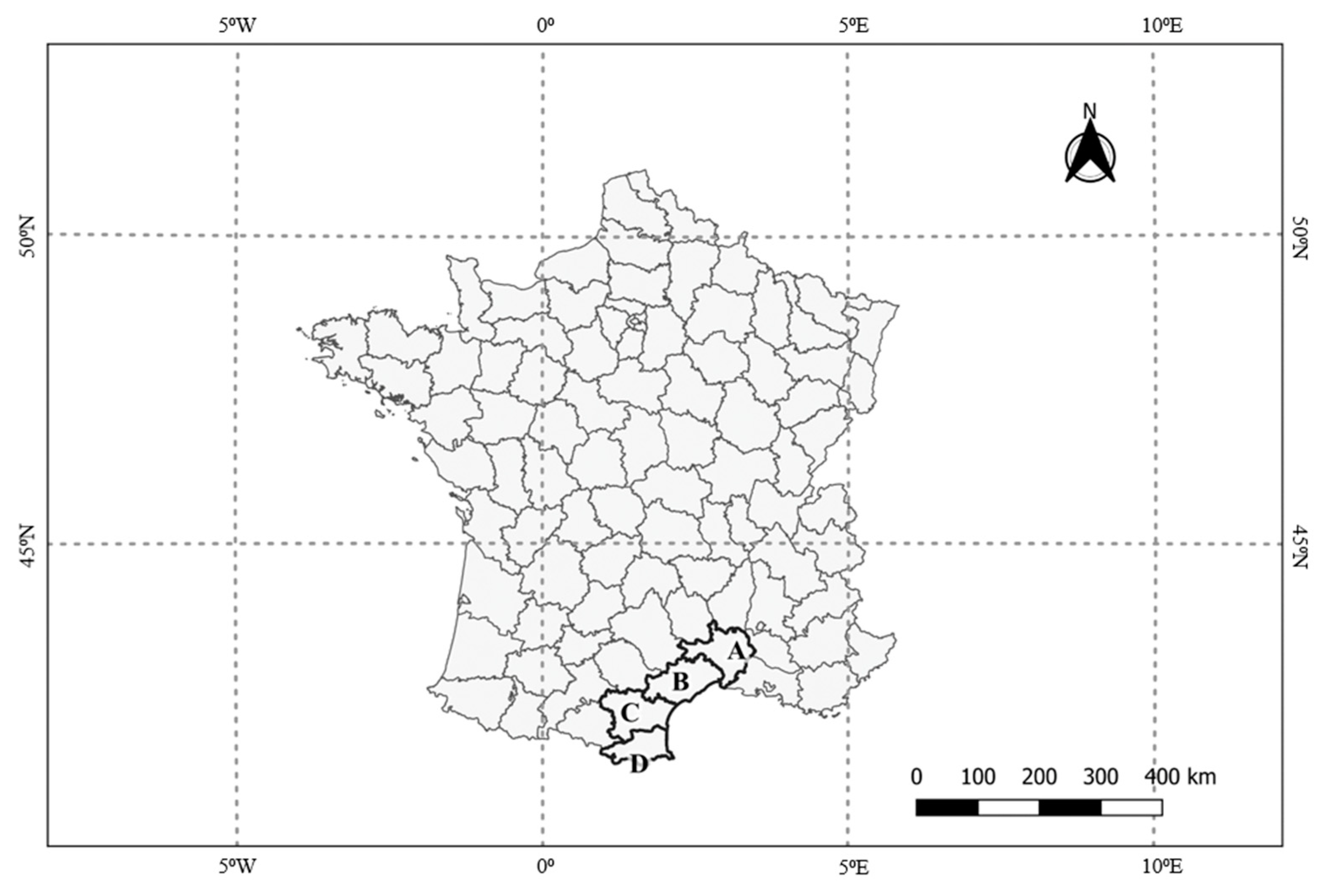
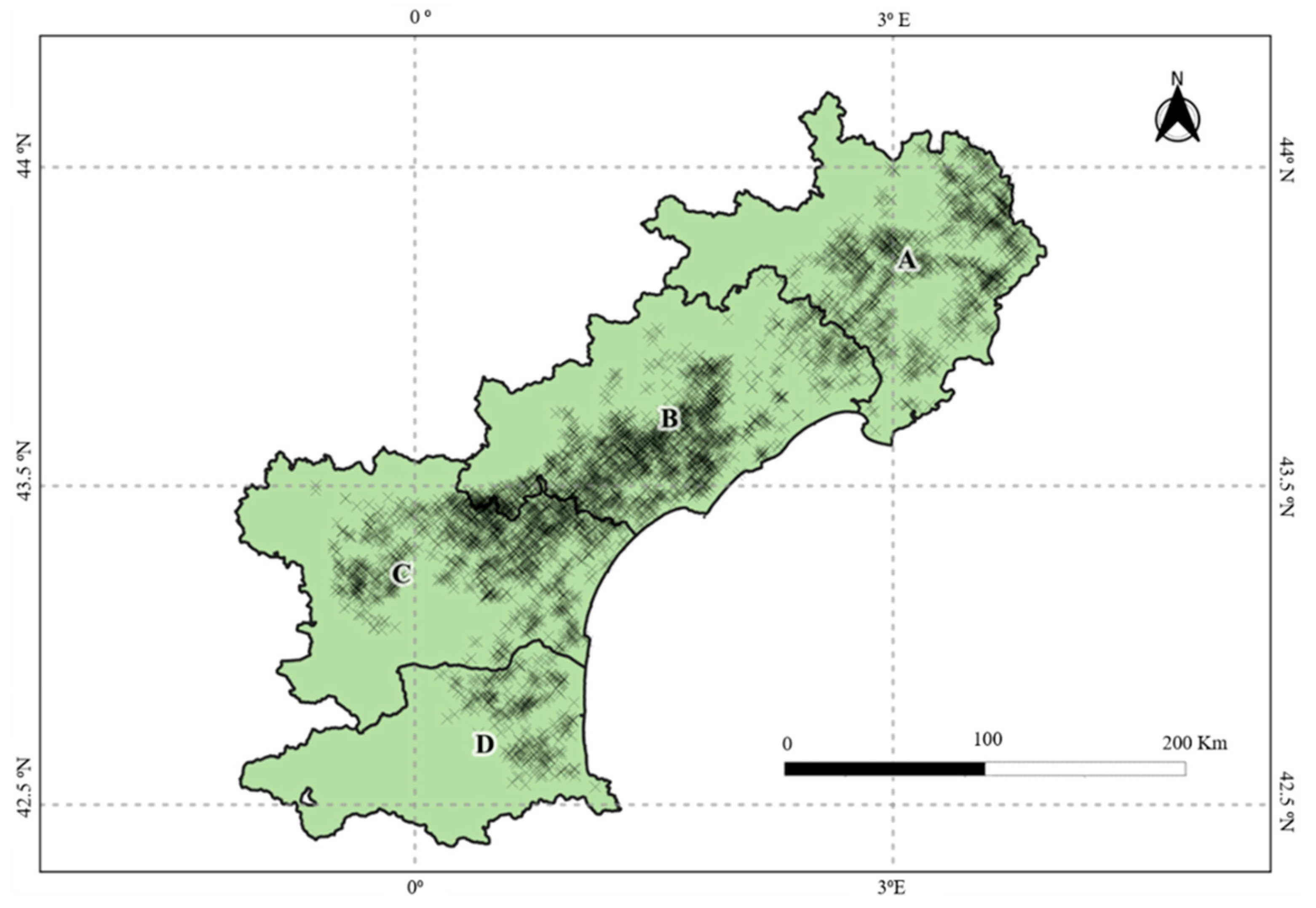
2.1. Study Area

The study area corresponded to a large vine growing region, the Languedoc-Roussillon (LR), extending over almost 27,400 km² in the south of France (Figure 1). The LR vineyards, united under the same administrative label but with their own characteristics, cover four French administrative sectors: Gard (A), Hérault (B), Aude (C) and Pyrénées-Orientales (D) (Figure 1). It encompasses a large diversity of varieties, training systems, etc. [16].

The climate, typically Mediterranean, is characterised by hot and dry summers, with sparse summer rainfall and mild winters. The regional level presents a large variability in pedo-climatic conditions [16]; however, soils typically share common characteristics: low fertility, high stoniness, good drainage, absence of a limiting horizon to ensure deep rooting and limited water holding capacity.

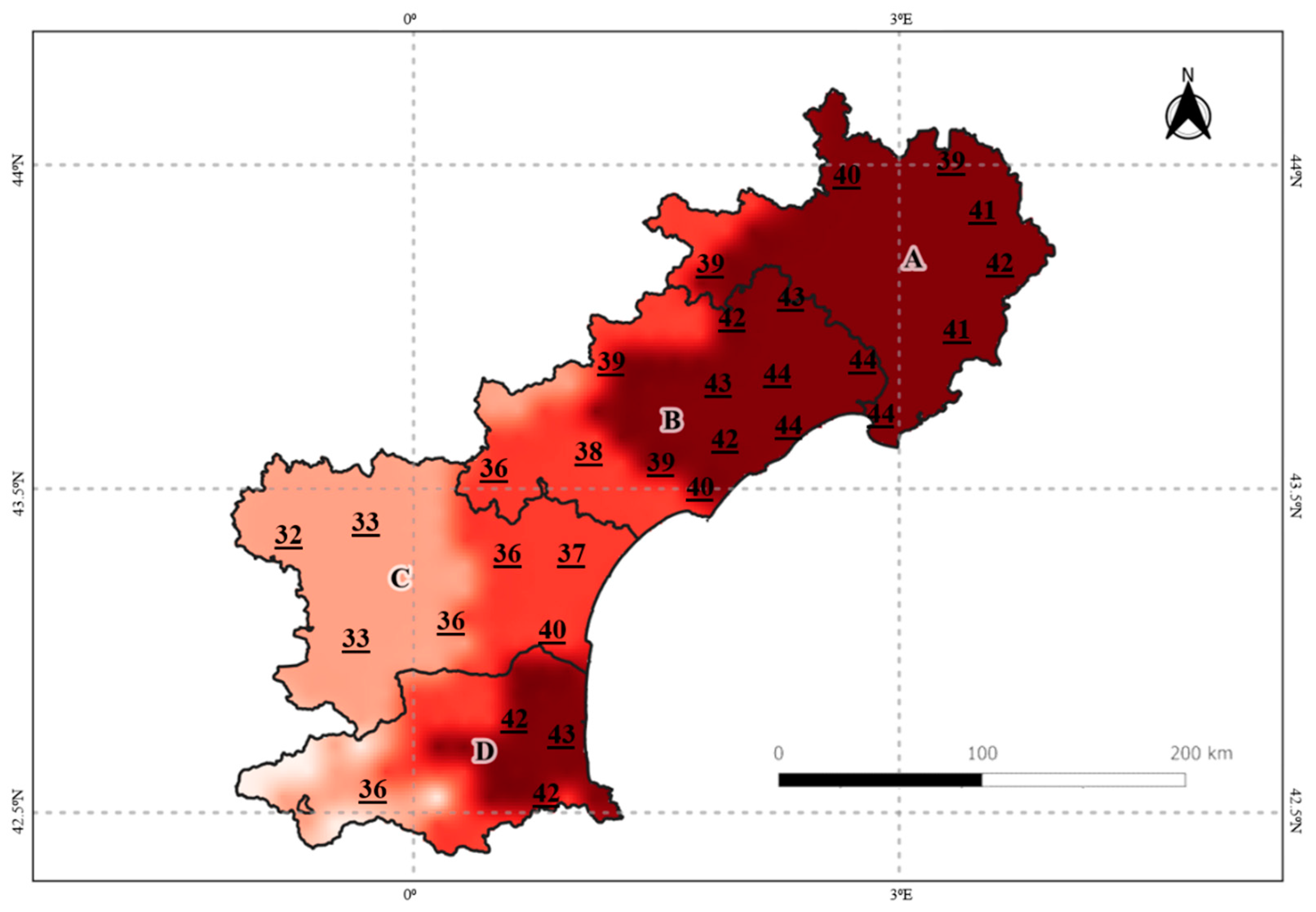
2.1.1. Heatwave Stress Characteristics

In June 2019, the LR wine-growing area experienced a heatwave characterised by a hot wind, blowing from the north-east to the south-west, with temperatures reaching 45 °C (Figure 2). The extreme weather episode occurred between 25 June and 8 July 2019, of which 28 June was the most critical day. Given that vine growth in Mediterranean conditions is still occurring, although slowing, in the middle of the season, extreme environmental fluctuations that occur during this period at very rapid time scales will limit the evaporative cooling of the leaves and induce symptoms that can even lead to wilting of the leaves [17]. Extremely high-temperature regimes, characteristic of a heatwave, affect the biochemical and physiological processes necessary for the optimal development of the vine, especially for early ripening varieties [1].

It should be noted that the heatwave did not affect the whole region equally, as shown in Figure 3. The northern part of the region (sectors A and B) was the most strongly affected. Indeed, sector B presented the highest maximal temperature (>44 °C), with a strong spatial variability, since these high temperatures did not affect the eastern part. Sector D was only severely impacted on the western part, and section C was almost unaffected by high temperatures. Note that Figure 3 only presents the main trend of the heatwave. It may hide some local (short range) phenomena due to factors that may locally mitigate or amplify the temperature effect experienced by vineyard blocks, such as elevation, the presence of forest and the aspect of the topography.

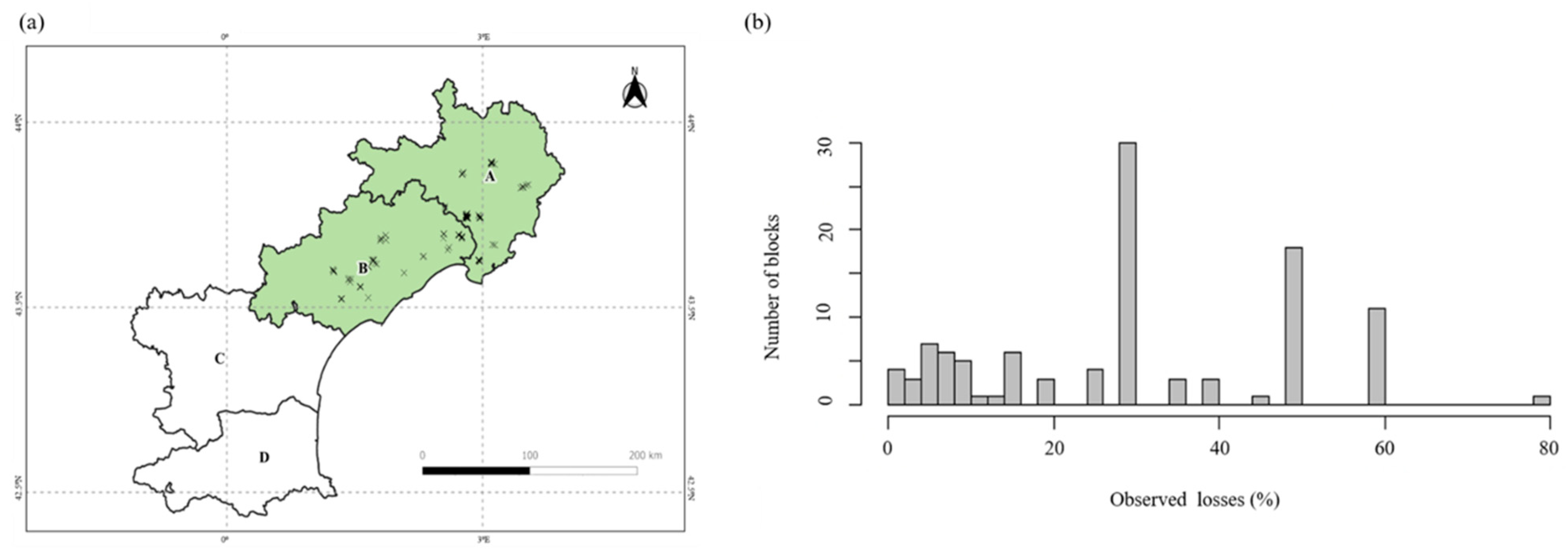
2.1.2. Ground Truth Data

The ground truth data were selected from 107 non-irrigated vineyard blocks in the northern part of the LR region (Figure 4a). They all showed some effects related to the heatwave, such as stalled development, leaf burn and leaf drop [18]. The severity of this effect was assessed by winegrowers and advisors on each of the 107 vineyard blocks several weeks after the event through an estimation of percentage of yield loss. Figure 4b summarises the distribution of the 107 blocks in relation to yield loss. Note that the ground truth data concerned only sectors A and B, which were the most impacted by high temperatures during the heatwave. No vineyard blocks were sampled over sectors C and D, despite the potential impact of the heatwave on both of these sectors. However, this unbalanced spatial distribution of the blocks leads to a representative dataset with a large diversity of observed yield loss values (Figure 4b).

2.2. Remote Sensing Data

Data Acquisition and Processing

Satellite images were selected via the Google Earth Engine (GEE) platform, which provides Sentinel-2 L2A (Sentinel-2A and Sentinel-2B) products. Sentinel-2 satellites, with a revisit frequency of 10 days (5 days with the twin satellites (A/B) together), provide 13 spectral bands from visible (Vis) and near-infrared (NIR) to shortwave infrared (SWIR) regions of the spectrum, with a spatial resolution of 10, 20 and 60 m (

Table 1. Spectral bands for the Sentinel-2 satellite considered by the analysis.

Sentinel-2 Band	Central Wavelength (nm)	Bandwidth (nm)	Spatial Resolution (m)
Band 1–Aerosol	442.7	21	60
Band 2–Blue	492.4	66	10
Band 3–Green	559.8	36	10
Band 4–Red	664.6	31	10
Band 5–Vegetation Red Edge	704.1	15	20
Band 6–Vegetation Red Edge	740.5	15	20
Band 7–Vegetation Red Edge	782.8	20	20
Band 8–NIR	832.8	106	10
Band 8A–Vegetation Red Edge	864.1	21	20
Band 9–VNIR	945.1	20	60
Band 11–SWIR	1613.1	91	20
Band 12–SWIR	2202.4	175	20

) [18]. Twelve spectral bands (among the 13 available from Sentinel-2 satellites) were used in this study (Table 1). Spectral band 10 at 1380 nm was not used as it was designed for the detection of visible and sub-visible cirrus clouds and corresponds to a band of high atmospheric absorption [19].

The time period considered for the study was from May to August 2019, which was the most relevant period to monitor vine growth vegetation in this region [20]. Only images containing the study vineyards (Section 2.1.2) from 13th May to 20th August 2019 were selected and processed via Google Earth Engine (GEE) [18]. Blocks’ boundaries were extracted from the graphical parcel register of France (RPG). According to the highest spatial resolution of Sentinel-2, to avoid mixed pixels, a 10 m inner buffer was imposed over the boundary of each block before average pixel values were computed within the inner boundary for each block, each date and each waveband [18]. For the chosen period, 25 images should have been potentially available over each block, but following the cloud detection algorithm for Sentinel-2 imagery proposed by Hollstein et al. [19], the number of available images was 11 on average, with a range from 7 to 16 images depending on the location of the different blocks [18].

2.3. Modelling

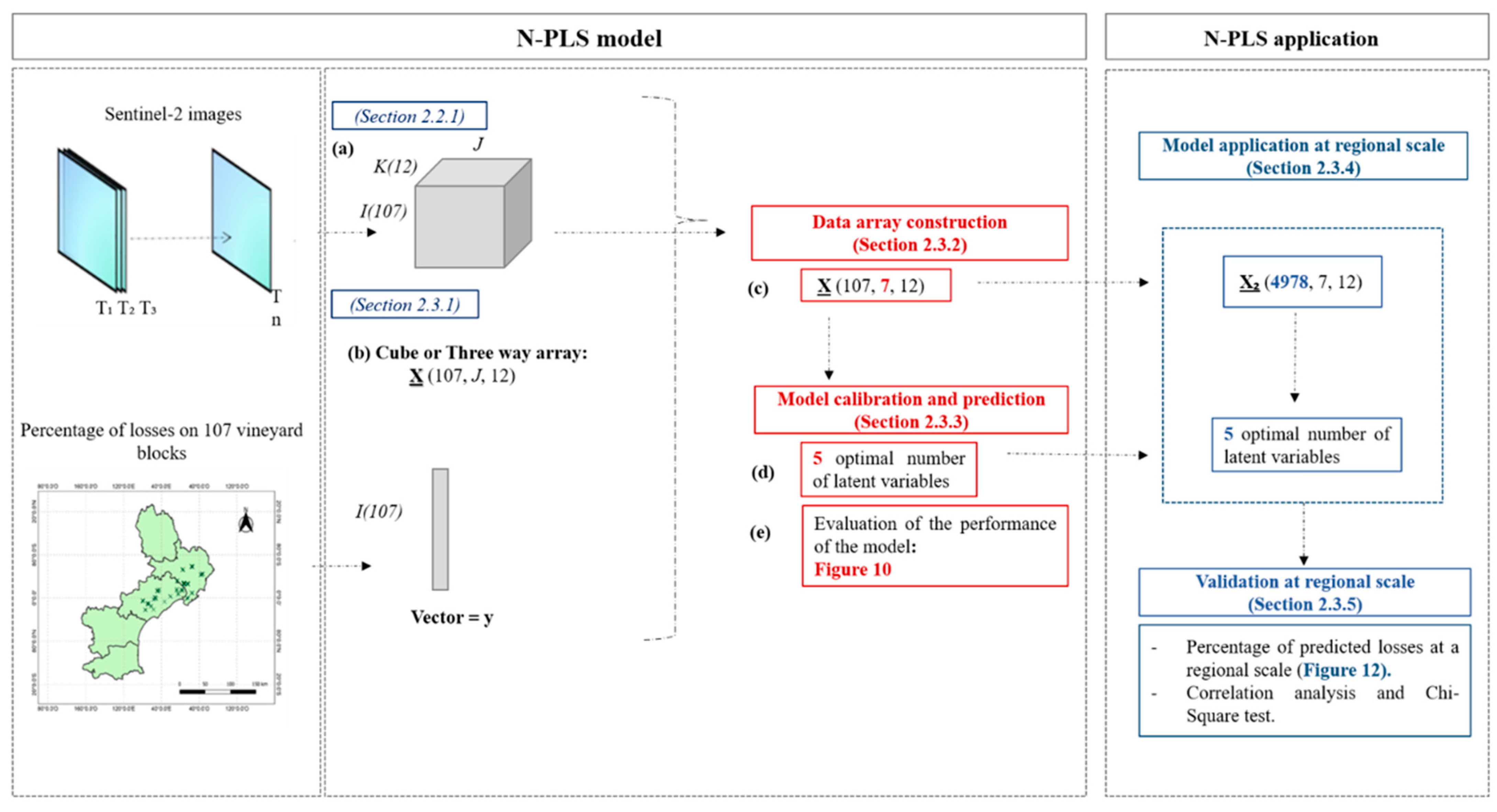
2.3.1. N-Way Partial Least Squares

In this work, data corresponded to a three-way array X = || X_i,j,k | whose dimensions involved the individuals (I), i.e., the vine blocks, as a first dimension, the second dimension corresponded to time (J) and the third dimension corresponded to mean reflectance at each wavelength (K). Therefore, as shown in Figure 5, data were organised in a three-way array of independent variables X (I × J × K) derived from the remotely sensed data (Section 2.2) and a response vector y of size (I × 1) corresponding to the ground truth data (Figure 4a).

N-PLS regression, as an extension of the classical partial least squares (PLS) method, was chosen to analyse the data. As proposed by Hansen et al. [21], it is an interesting method to relate a N-way array to a dependent variable. It identifies all latent information from (X), which maximises the covariance between X and y while keeping information provided by each dimension of X [22]. In this study, the 3-PLS1 regression method [23] was used to best relate X with y while keeping information provided by the spectral and the temporal dimensions.

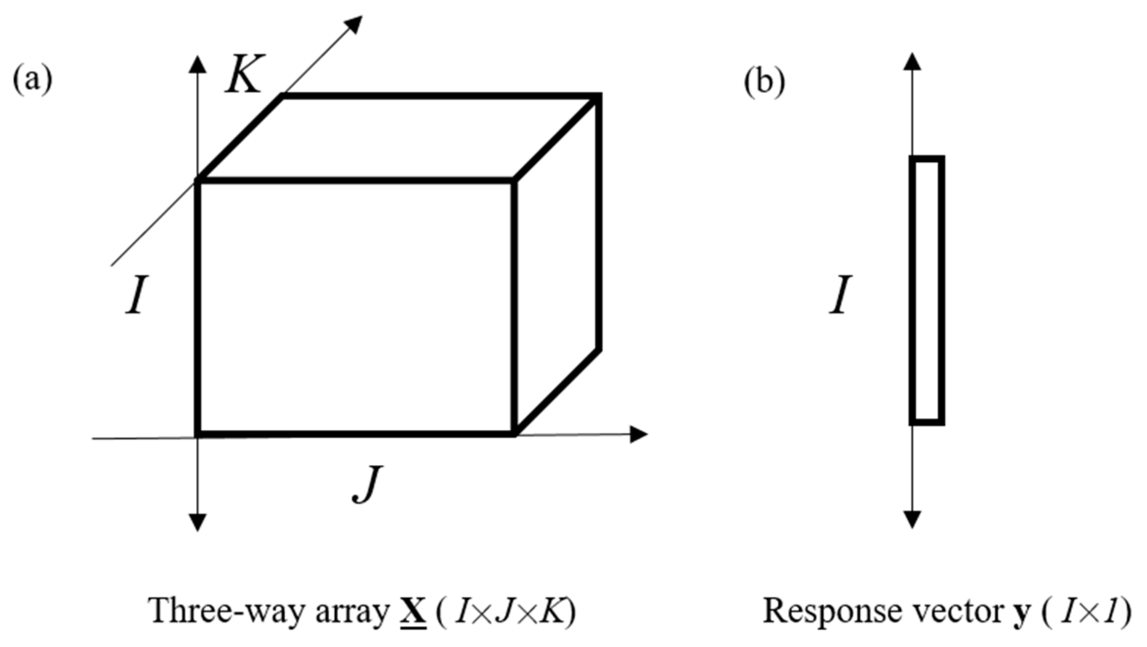
2.3.2. Data Array Construction

The dataset was characterised by the observations of the 12 spectral bands averaged over each of the 107 blocks for all available satellite images, between 13 May and 20 August, in 2019 [18]. However, the number of images per block varied according to the local atmospheric conditions over each block for each acquisition date. As a result, all potential Sentinel-2 images were not necessarily available at each date. To overcome this issue, an interpolation was performed to obtain a continuous data cube. The interpolation at a date t was done wavelength by wavelength, by a convolution of the chronology measured with a Gaussian filter [24] in order to have a consistent time step dimension (J) [18]. The parameters involved in the interpolation setting were optimised by cross-validation of 2 blocks repeated 5 times of a N-PLS between cube X and vector y. Parameter optimisation was achieved with a Gaussian filter having width (P) = 30 and date interval (N) = 15 [18].

At the end of the interpolation step, the dataset was meaningfully arranged in a three-way array X of dimensionality 107 (samples, I) × 7 (times, J) × 12 (wavelengths, K) and a vector y (107), corresponding to the yield loss rates from 107 blocks estimated by the winegrowers and advisors.

2.3.3. Model Calibration and Prediction

Calibration and validation subsets were created to build and evaluate the model. Considering the distribution of the samples from the dependent variable (Figure 4b), a calibration set (3/4) and a validation set (1/4) were defined as follows to ensure that the two sets had the same final distribution [18]:

(1)

The vector y was sorted in ascending order.

(2)

After sorting, every fourth individual was placed in the validation set and the others were kept in the calibration set.

A cross-validation of 2 blocks repeated 10 times of a N-PLS between the X cube and the y vector from the calibration set was performed. The joint analysis of the Root Mean Square Error of Calibration (RMSEC) and the Root Mean Square Error of Cross-Validation (RMSECV), as proposed by Goodarzi et al. [25], was used to determine the optimal number of latent variables (LVs) in the regression model. On the basis of this joint analysis, 5 meaningful latent variables were kept for the model [18].

The prediction performance of the model was quantified on the validation subset (data not used for the model calibration) by the standard determination coefficient R², the bias and the standard errors.

2.3.4. Model Application at Regional Scale

In order to assess the potential of the approach in identifying the spatial footprint of the heatwave phenomenon at the regional scale, the calibrated N-PLS model was applied to 4978 vineyard blocks spread over the whole LR region (Figure 6). These vineyard blocks corresponded to all data available from the RPG.

For the implementation of the N-PLS model, the same steps were followed as for X data array construction (Section 2.3.2.). The model with the 5 latent variables (Section 2.3.3.) was therefore applied to a significant three-way array X₂ of dimensionality 4978 (samples, I) × 7 (times, J) × 12 (wavelengths, K). The model application provided an estimation of the yield loss over the 4978 vineyard blocks.

Figure 7 summarises the implementation and the workflow scheme of the N-PLS model calibration, in addition to its validation and its application at the regional scale.

2.3.5. Validation at the Regional Scale

Yield loss estimations at the regional scale were interpolated following a classical kriging process (Section 2.4). Estimations were analysed both qualitatively from visual comparison with the maximum temperature record map of the 28 June 2019 (Figure 3), and quantitatively, based on the occurrence of predicted yield loss values with respect to the maximum temperature recorded over the block. As validation, a chi-square test of independence [26] was used to verify the dependency between both information sources at the regional scale. The H₀ hypothesis was that yield loss estimation was independent of maximal temperature recorded during the heatwave event. H₀ was rejected for p-values of 0.05 (p < 0.05).

Both estimated yield loss and temperature values are continuous variables. In order to account for inaccuracy and short-range variability, both variables were converted into classes to carry out the test. For yield loss estimations, the width of the classes was defined from the data distribution at the regional scale, i.e., it was based on the distribution of predicted values [27]. For the temperature values, a theoretical criterion was applied. Fraga et al. [7] stated that during critical periods of vine development, e.g., in the growth period, if the air temperature reaches a threshold above 35 °C, a limitation of photosynthesis is to be expected, leading to a decrease in productivity. Therefore, it was decided to set a threshold temperature at 35 °C and to establish two classes above and two classes below this threshold. The widths of the 4 classes were determined by (1) the temperature threshold and (2) the minimum and maximum temperature recorded on the 28th June 2019.

2.3.6. Model Interpretation

As for the classical partial least squares (PLS) method, the three-way PLS model aims at finding new components called latent variables (LVs), which best relate data X (samples × time × wavelengths) to y (ground truth data) [22]. Compared to classical PLS, the three-way PLS allows the information supported either by the time dimension or the spectral dimension to be kept and analysed properly. The weight vectors of each LV correspond to a spectral and temporal profile, providing evidence on the spectral bands and their dynamics over time that may best explain the yield losses. The most relevant LVs (i.e., those that best explained yield loss) were then selected and analysed to identify known information supporting the model performance, in addition to new complementary knowledge provided by the time series of images to characterise the heatwave. The standard error of prediction (SEP) [28] was used to determine the LVs to be analysed.

In addition to the LV weight vectors, the score of each of the 4978 blocks was calculated for each LV. The score value of a block shows its relation to the spectro-temporal profile defined by the LV. Then, 3 cases were considered:

• if the temporal-spectral profile of a block followed the same signature as the one created from the weight vectors (temporal and spectral bands) of a LV, the score value was positive;
• if the temporal-spectral profile of the sample (vineyard block) followed the inverse signature to the one created from the weight vectors (temporal and spectral bands) of the LV, the score value was negative; and
• if the temporal-spectral profile of the sample (vineyard block) followed a different signature to the one created from the weight vectors (temporal and spectral bands) of the LV, the score value was close to zero.

2.4. Mapping and Spatial Analysis

Maps were obtained using point kriging interpolation. Kriging was performed with the GeoFis 1.0 software [29], which was used for: (1) the modelling of semivariograms and calculations of their featured parameters, C₀ (nugget effect), C₁ (sill) and r (range), and (2) the kriging interpolation. The latter was performed on a grid of regularly spaced points 1000 m apart within the geographical boundary of the LR region.

Semivariogram features were also used to compute the Cambardella Index (I_c) [30] (Equation (1)):

$${\mathrm{I}}_{\mathrm{c}}=\frac{{\mathrm{C}}_0}{{\mathrm{C}}_0+{\mathrm{C}}_1}$$

(1)

where C₀ is the nugget effect and C₁ is the sill of the semivariogram model. The Cambardella Index was considered here to quantify how the data were organised spatially over the LR region. The common following thresholds were then used: (1) I_c less than or equal to 25%, the distribution is considered strongly spatially organised; (2) for I_c between 25 and 75%, the distribution is considered moderately spatially organised and; (3) if I_c is higher than 75%, the distribution is considered weakly spatially organised [30,31].

3. Results

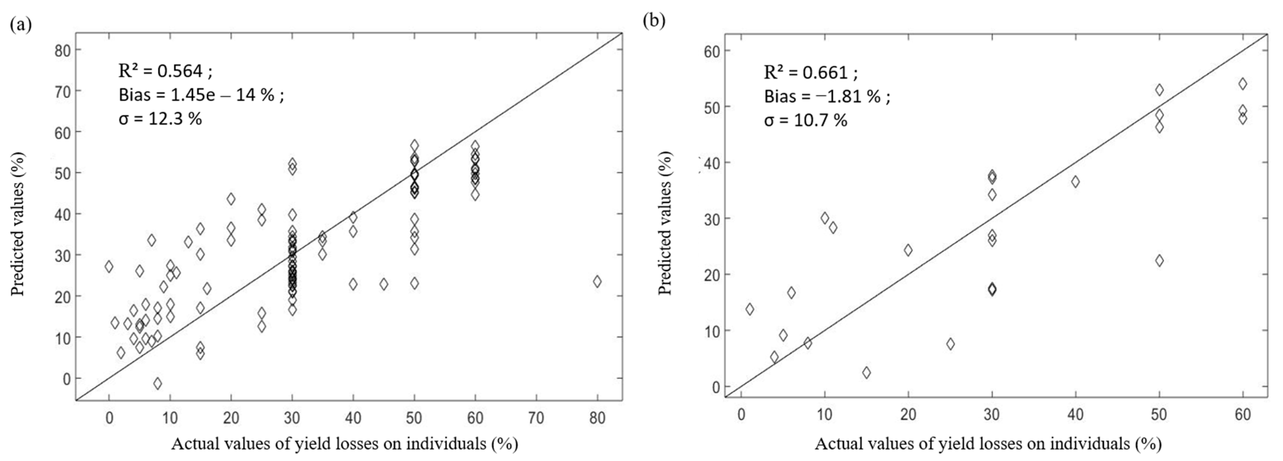
3.1. Quality of the N-PLS Model

The performance and quality of the N-PLS model with five latent variables are presented for the calibration set (Figure 8a) and validation set (Figure 8b) in terms of R², bias and standard error of prediction of yield losses. The N-PLS model showed a performance accuracy (R²) of 0.56 in the calibration set and of 0.66 in the validation set, with a standard error of cross-validation in the calibration set of 12.4% and a standard error of prediction of losses in the validation set of 10.7% [18]. A standard error of 10.7% over the prediction set (Figure 8b) was consistent with the accuracy level of the ground truth data, which gave the yield loss in 25% classes (Section 2.1.2).

These results prove the relevance of multispectral satellite time series to assess the incidence of a heatwave on grape vine loss when combined with the N-PLS. However, this model was only validated on a small number of vineyard blocks spread over a small representative part of the region. The next sections aim at verifying whether the model derived from this small dataset could be applied to the whole regional level in order to verify its ability to highlight heatwave footprint at this scale.

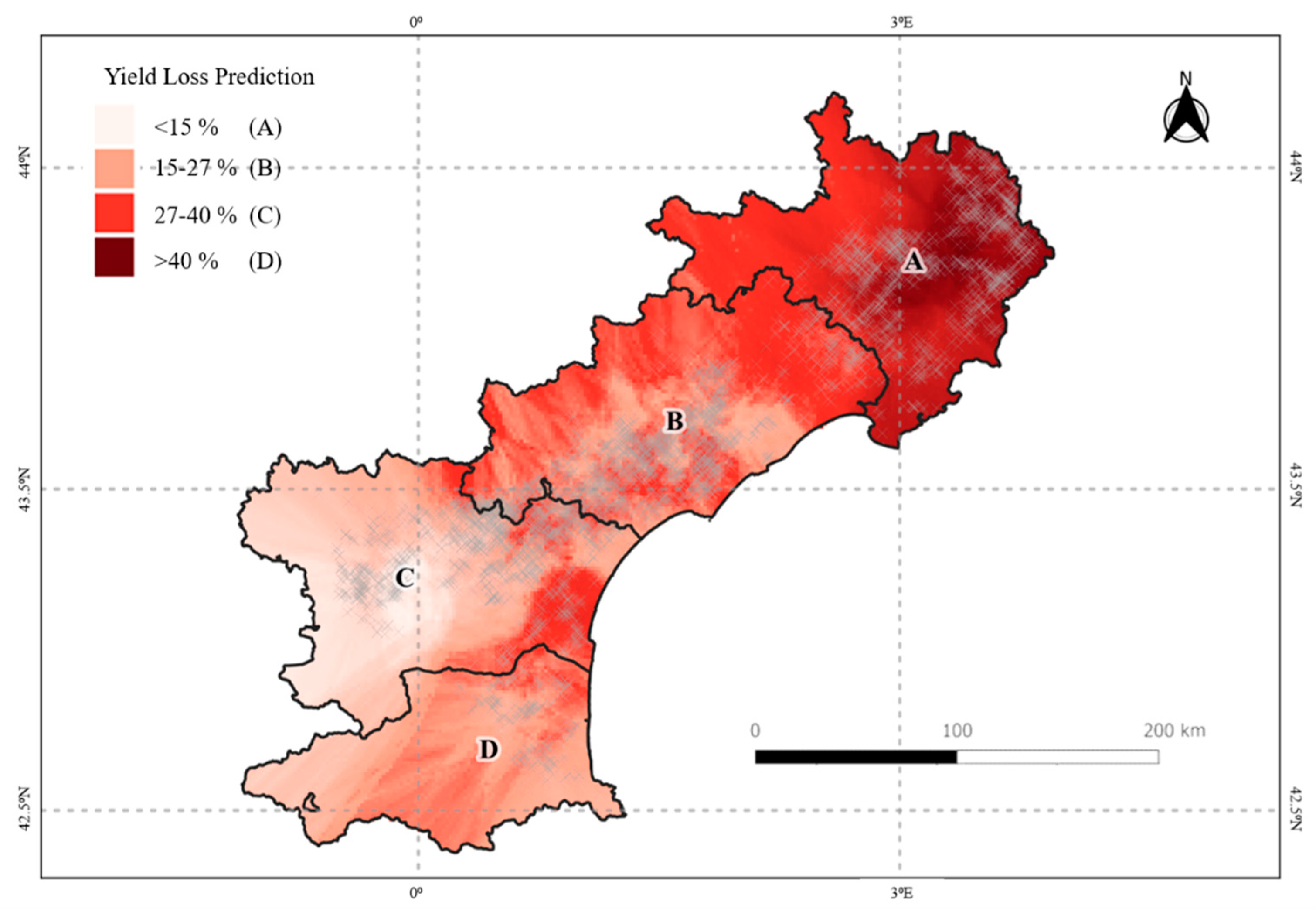
3.2. Yield Loss Prediction at the Regional Level

Figure 9 shows the distribution of the yield loss prediction when the N-PLS model calibrated with the 107 vineyard blocks is applied to 4978 vineyard blocks of the region. From the mean (μ) and the standard deviation (σ) values of the distribution, four classes of yield loss were defined as follows: predictions between 0 and 15% yield loss represented a low impact (a), predictions between 15 and 27% of losses represented a moderate impact (b), predictions between 27 and 40% of losses represented a high impact (c), and predictions > 40% represented a severe impact of heat stress (d).

Figure 10 shows the kriged map of the yield loss prediction at the regional scale. The kriging was performed with a Gaussian semivariogram model, with a nugget effect (${\mathrm{C}}_0)$ of 122, a sill $\left({\mathrm{C}}_1\right)$ of 175 and a range of 140 km. The Cambardella index (I_c) resulting from this semivariogram was 41%, which highlighted a (moderate) spatial organisation of yield loss predictions, i.e., 41% of the variability exhibited a spatial structure while the remaining variability (59%) was stochastic in nature.

The kriged map (Figure 10) shows large spatial patterns that are more or less related to patterns observed on the maximal temperature map (Figure 3). Indeed, it highlights two main zones, one in the northern part (A and B) corresponding to a high yield loss in the majority of the area, and the second in the southern part (C and D), with a lower yield loss. This main trend was clearly in relation with the maximal temperature map (Figure 3), which exhibited the same patterns. The kriged map also exhibited local patterns showing some local variations in yield loss. This was clear for sectors B and C, where smaller zones of yield loss were clearly highlighted.

In order to validate the qualitative observations made from the kriged map, a quantitative analysis of the results was proposed. Given the difficulty of obtaining reliable ground truth data at this scale, the proposed validation was based on the analysis of a contingency table between the yield loss classes with classes of maximum temperature observed on the day of the heatwave (

Table 2. Contingency table cross-referencing the yield loss prediction classes with the maximum temperature classes recorded on 28th June 2019.

	(30–32.5 °C)	(32.5–35 °C)	(35–40 °C)	(40–45 °C)
Low impact: (0–15%)	333	0	0	0
Moderate impact: (15–27%)	417	552	0	0
High impact: (27–40%)	0	1289	704	0
Severe Impact: (40–80%)	0	0	749	934

). The same classes of yield losses were considered as for the kriged map.

Table 2 shows a clear relationship between the variables, and this relationship was clearly positive, i.e., the number of blocks impacted by the heatwave increased with the maximal temperature at the regional scale. The H₀ hypothesis (independence of data distribution within the contingency table) tested with a classical chi-square test was rejected (p-value < 0.01). Therefore, classes of estimated yield losses were significantly related to the heatwave at the regional scale.

Note that the results obtained are very specific. The model did not estimate a significant loss of yield when the recorded maximum temperatures were relatively low (<32.5 °C). On the contrary, when the recorded maximum temperatures were very high (>40 °C) the model estimated very high yield losses. Table 2 also highlights some inaccuracy between yield loss classes; for example, the 32.5–35 °C temperature class can lead to moderate and large predicted yield losses. This observation should be considered in the light of the definition of the classes, which were only roughly defined on the basis of the overall distribution of the data and which would certainly merit from adjustment according to the zone of the region, or according to the grape varieties, training systems, management practices, etc. It should certainly be considered in the light of the important nugget effect, which may be explained by a high inter-block variability (grape variety, block aspect, micro-topography, etc.) when working at this scale.

These results demonstrated the relevance of the model (derived from N-PLS) when applied at the regional level to predict yield losses associated with the heatwave of 28 June 2019. Based on these insights, the kriged map presented in Figure 10 may represent a relevant spatial footprint of the heatwave impact of grape yield losses at the regional level.

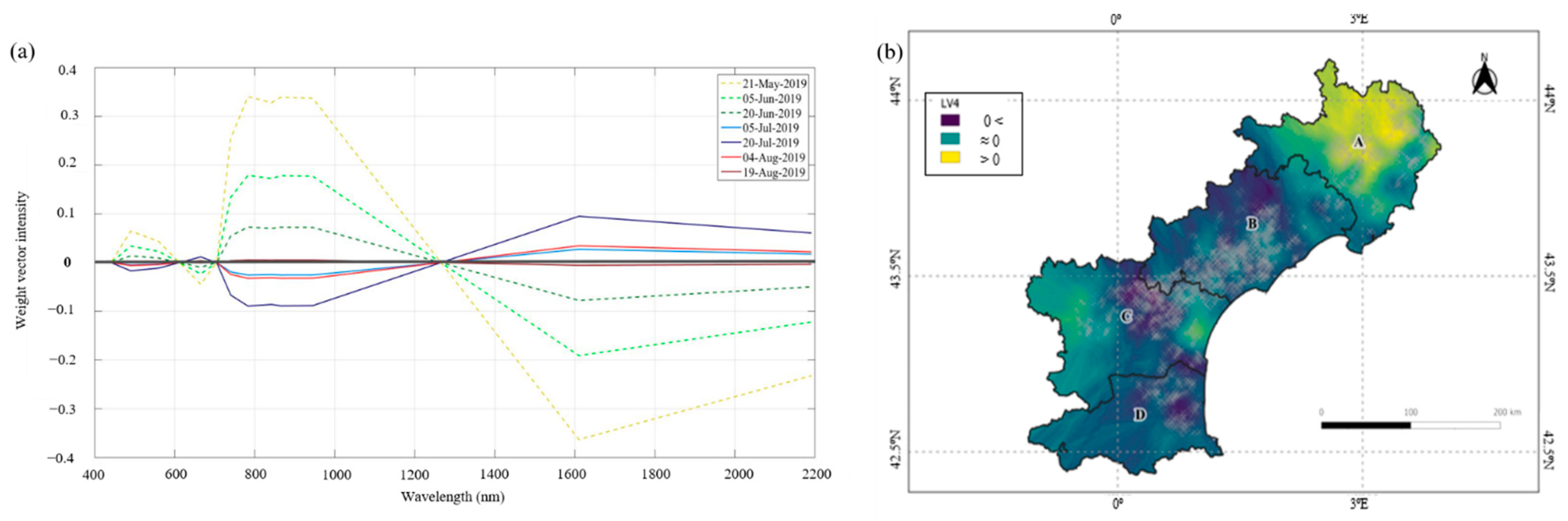
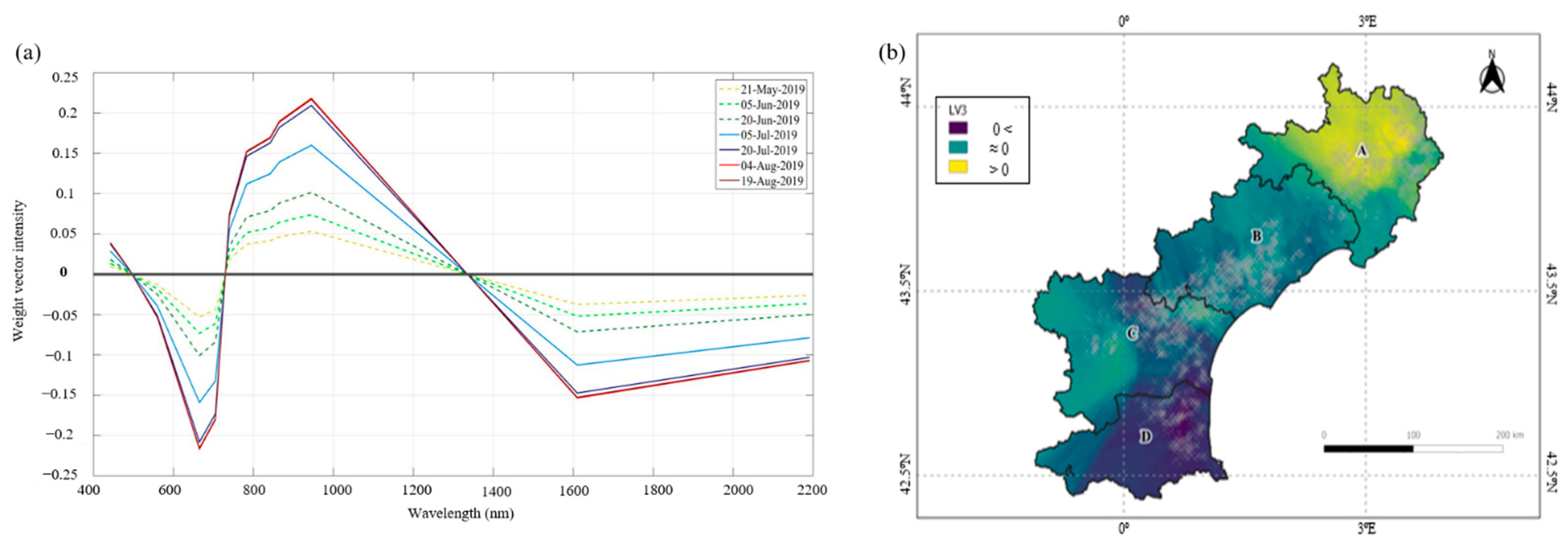
3.3. Insights of Time Series and Spectral Analysis of the N-PLS Model

Table 3. Standard error of prediction (SEP) for each of the five latent variables derived from the N-PLS model on the calibration set.

LV1	LV2	LV3	LV4	LV5
1.52	1.20	−1.06	−0.04	−1.81

shows the standard error of prediction (SEP) of yield loss for each LV derived from the N-PLS. [32]. LV3 and LV4 were the LVs that best predicted the yield loss (lowest SEPs). Therefore, the next section focuses on studying, first, the LV4 that presented the lowest SEP (−0.04), and, in a second step, the LV3 that showed the second lowest SEP (−1.06). The LV4 and LV3 were analysed thereafter regarding their relevance towards the yield loss estimation.

Figure 11a presents the weight vectors of LV4 as a spectro-temporal profile, i.e., for each date. The weight vectors can be viewed as the bands that most impact the vine response in relation to the heatwave. It showed several interesting patterns: (1) for reflectance between 800 and 1000 nm, high weights were observed at the beginning of the season (May), whereas low (negative) weights were observed right after the heatwave (5 July), and the weights decreased again until the end of July and then increased until end of August; (2) for reflectance between 1600 and 2200 nm, the opposite trend was observed, with low weights (negative) at the beginning of the season and high weights after the heatwave (5 July), and the highest weights were observed a few weeks (20 July) after the heatwave. Reflectances between 750 and 1350 nm are known to be strongly related to leaf structure [33], whereas reflectances between 1350 and 2200 nm are strongly linked to water absorption [34]. Both of these ranges of reflectance were strongly impacted from immediately after, until three weeks after, the heatwave. Therefore, the spectro-temporal profile of LV4 summarised the dynamic of the incidence of the heatwave on the vineyards’ canopy. The LV4 weights showed that this may result in a drastic change in canopy structure partly due to a change in water content a few weeks after the event. Note that LV4 weights also highlighted the slow recovery of the canopy after 20th July for these wavebands.

The score values (Figure 11b), represented the agreement between the LV4 weights and the spectro-temporal profiles of each block. The score map obtained after kriging describes the spatial organisation of the blocks that present: (i) similar spectro-temporal profile (score > 0); (ii) opposite spectro-temporal profile (score < 0); and (iii) no related spectral-profile (score ~ 0). The score map for LV4 was supposed to highlight blocks that were directly impacted (or not) by the heatwave. The spatial organisation of the scores was confirmed by the semivariogram model, which showed (

Table 4. Semivariogram parameter descriptors and spatial variability index for score values ${\mathrm{A}}_1$ (Range), ${\mathrm{C}}_0$ (Nugget), ${\mathrm{C}}_1$ (Sill) and ${\mathrm{I}}_{\mathrm{c}}$: Cambardella Index.

Latent Variables	Semivariogram Model	Range (Km)	C₀	C₁	Ic (%)
Scores LV3	Spherical	17	0.011	0.019	29
Scores LV4	Gaussian	27	0.003	0.004	48

) that around 50% of the variability was explained by a spatial phenomenon (I_c = 48%). The spatial patterns were strongly related with the maximal temperature recorded on 28th June, showing that the blocks of the northern part of the region were in agreement with the LV4 spectro-temporal profile. Note also that, for other sectors, patterns were less related to the main trend of the heatwave. Blocks with a score > 0 underwent a drastic change in canopy structure, partly due to change in water content a few weeks after the heatwave. Patterns of strongly impacted blocks can also be seen in sectors B and C. Note, however, that for sectors other than sector A, the patterns were less related to the main trend of the heatwave.

LV3 showed an unusual trend with regard to the common evolution of the vine canopy over the season (Figure 12a). It had the highest weights (positive or negative) at the end of the season, from the July, and especially in August, when growth has usually stopped and canopy reflectance should be relatively stable (until senescence onset). These high weights corresponded to (1) the 664 nm reflectance (negative weights), (2) reflectances between 800 and 1000 nm (positive weights), and (3) to a lesser extent, reflectances between 1600 and 2200 nm (negative weights). They corresponded respectively to (i) the visible spectrum (400–700 nm), which is affected mostly by photosynthetic pigments content (chlorophyll and carotenoids), (ii) leaf and canopy structure (750–1350 nm) and (iii) water content (1350–2200 nm) [35]. The highest ranges of reflectance (positive or negative) reached their maximum long after the heatwave episode (between 20th July and 19th August). Thus, LV3 weights may represent vines that were strongly affected by the extreme weather episode and that recovered their photosynthetic capacity of part of their leaf canopy later in the season [36].

The score map for LV3 (Figure 12b) was expected to highlight, on the one hand, blocks showing biomass growth after the heatwave (score > 0) and, on the other hand, blocks showing the opposite phenomenon (score < 0), i.e., an increase in photosynthetically active biomass in spring (before the heatwave) and a stabilisation or even a decrease in August (which should correspond to the expected behaviour of vines in normal conditions). The spatial organisation of the scores was confirmed by the semivariogram model used to krige the scores (Table 4), with around 70% of the variability explained by a spatial phenomenon (I_c = 29%). The spatial patterns showed a distinct north–south difference in the LR region, which again corresponded to the maximum temperature patterns recorded on 28th June 2019, and thus to the vineyard blocks most affected by the extreme event.

4. Discussions

This study demonstrated the potential of temporal series of multispectral remote sensing images to discriminate and characterise the impact of a heatwave on vineyards at a regional scale. It also demonstrated that the high dimensionality (temporal and spectral) of the data required adopting a systemic methodology that accounted simultaneously for the spectral and temporal characteristics of the considered data. The N-PLS (3-PLS1 in our case) may be considered as a relevant approach to handle such problems. It allowed the spectral and temporal dimension of the data to be considered simultaneously in order: (i) to calibrate a model of prediction and (ii) to keep information captured by the spectral and the temporal dimensions through latent variables, which provided insights into the changes undergone by vine canopy.

The approach, although calibrated on a few fields, was successfully applied at the regional level, showing the robustness of the methodology and its ability to map the spatial footprint of the heatwave that affected the south of France in 2019.

It is essential to place the results presented in this paper within the reality for many environmental and agricultural studies where the ground truthing remains weak and hard to manage. The N-PLS model shows the interest in successfully dealing with a low number of ground truth samples (in this case, 107 yield loss observations for grape fields). Nevertheless, it should be noted that the N-PLS model here was still specific to the learning base used for the calibration. Specifically, the model accounted for the timing of the heatwave that the dataset, used for the calibration, had undergone. The direct application of the model to other vintages or to other regions should then not be considered. Despite this limitation, the approach allowed the identification of spectral changes in canopy reflectance that may be the signature of an early summer heatwave. This signature can be applied, with expert set up, to other case studies in order to identify potential heatwave effects when no ground truth data are available. Another limitation is that the model integrated the whole season dynamic (from May to August). As a result, it is not suitable to be used as a monitoring model to identify and spatialise the heatwave effects in real time or even a few days after the event.

Although this study focused on the assessment of grapevine heat stress at the regional level, the generation of potential knowledge from a multispectral time series with the intention of understanding the phenomenon in question (i.e., a heatwave), was achieved through the N-PLS approach. Previous studies have shown significant abilities to assess the effects of heatwaves [3,13] by evaluating the physiological and spectral responses of grapevines. Notwithstanding this, the adoption of a PLS-multiway analysis presents the advantage of accounting for changes in the spectral responses over time. Indeed, the two latent variables most representative of yield loss in the model (SEP values of −1.06 for LV3 and −0.04 for LV4) provided knowledge regarding heat stress in vineyards by means of weight and score values. LV4 defined the spectral response of the vineyards to thermal stress, marking a clear temporal evolution where all the spectral information was affected, thus reversing the “theoretical” vegetation profile. LV3 reported on the period after the heatwave. In this case, the spectro-temporal profile of LV3 generated insights related to the unusual vegetation growth observed in mid-August. A possible explanation for the late recovery of greenness could be the experience of the vineyards after the heatwave, as the north was the area most affected by the extreme climatic episode. However, the interpretation of the other LVs in relation to the heatwave remains more challenging. Indeed, the N-PLS aimed to extract LVs that best explained the output variable. For that purpose, it may generate LVs that first model general trends to better extract specific phenomena. As a result, the first LVs may be more related to the evolution of a “standard” vegetation canopy signature in viticulture. The analysis of LVs as proposed in this study remains difficult and requires further understanding of both the N-PLS approach and the phenomena under study.

The validation of the model at the regional scale was performed based on the maximal temperature observed on 28 June 2019. The use of only maximum temperature is a relatively simple approach for a very complex phenomenon. There is still some debate about how the impact of a heatwave on vineyards should be assessed and which factors need to be taken into account, such as the onset dates, the duration of the heatwaves [7], and humidity and the resulting vapor pressure deficits [37]. Similarly, summarising the effect of a heatwave to a yield loss, as was done in this study, is certainly reductive. Other response variables (vigour, chlorophyll content, etc.) would certainly have been interesting to consider and more directly related to remote sensing variables. However, from an operational point of view, yield loss was an integrative response of the vine plant and, moreover, important for the wine industry. Nonetheless, the statistical analysis of the relationship between the maximum temperature recorded on 28 June 2019 and yield loss predictions (p-value ≤ 0.001) showed that the model may have captured the main trend of the heatwave impact on yield at the regional scale.

At this regional level of analysis, it is unclear whether the small spatial patterns observed in Figure 10, on sectors B and C, are indeed local variations of the impact of the heatwave on the vine. Given the strong spatial structure observed, the results may support this hypothesis. Indeed, spatially structured environmental factors, such as soil type, elevation, aspect, etc. can explain local variations in heatwave characteristics (duration, maximum temperature, etc.), which would explain the local variations observed in predicted yield losses. It would be interesting to validate this hypothesis because, if it proves to be correct, the use of image time series associated with a fine mapping of meteorological conditions may be a powerful tool to better characterise the effect of meteorological conditions during a heatwave.

At the regional scale, a high nugget effect was observed, indicating that a significant proportion of the variance remained independent of spatially organised factors or was explained by very short-range phenomena. Other factors undoubtedly affected the change in spectral response of the vine canopy, such as the variety, the training systems and the management practices. For the record, the LR region presents a wide variety of rootstocks, cultivars and clones, in addition to different soil characteristics and training systems. Since the model was applied without considering these factors, they may explain the strong variability that was observed at very short ranges from one field to another. It is difficult to know if these factors affected the spectral response of the canopy or if they locally mitigated/amplified the effect of the heatwave as it was observed from remote sensing or both. This interrogation promotes interesting questions to study the potential of the temporal series of multispectral images to better study how field characteristics may drive the response to heatwaves [4,38].

The applied multidirectional approach (N-PLS) presented here represents a specific case of viticulture for the heatwave of 28 June 2019 in LR. In general, though, it is a type of approach that can be effective in characterising and assessing the impact of extreme weather events that suddenly affect the spectral response of the vine canopy, e.g., hail and frost, with a distinct, disrupted temporal evolution. However, its application to more gradual phenomena, such as progressive changes in water status or nutritional problems, may be less adapted as changes in plant characteristics may be less obvious.

5. Conclusions

This study demonstrated how, with a proper dimensionality reduction algorithm such as the N-PLS, a time series of multispectral images can provide an estimation of the impact of a heatwave on vineyard blocks at a regional level. The methodology proved to be relevant to provide the spatial footprint of the heatwave through its evolution over time by means of the observed response of spectral information.

The relationship between the percentage yield losses and the maximal temperature recorded on 28 June 2019 at the regional scale was shown. Insights into the phenomena explaining canopy responses were provided from the spectro-temporal signatures of the latent variables, showing the potential of the approach to provide knowledge on canopy changes during such an event. The main limitation of the proposed methodology was its necessary calibration on the spectral temporal signature of the event under study. This prevented any application of the calibrated model to other heatwaves whose timing would be different.

The proposed methodology is potentially transferable to other phenomena that evolve over time and, in particular, to any sudden climatic event that may affect the growth dynamics and leaf composition of the vine canopy (frost, hail, plagues to some extent, etc.). However, the approach seems less suitable for more gradual phenomena, such as plant water status, as the temporal evolution is less evident.

Further research is needed to identify and characterise the effects of factors affecting the specificity of the spectral temporal response of vine canopy towards a heatwave. This should provide a new methodology to better analyse incidences of heatwaves on canopy responses at a large scale, and the potential mitigating or amplifying effects, such as microclimate, topography, training systems and variety.

References

1. Droulia, F.; Charalampopoulos, I. Future Climate Change Impacts on European Viticulture: A Review on Recent Scientific Advances. Atmosphere 2021, 12, 495. [Google Scholar] [CrossRef]
2. Pinel, E.L.; Duthoit, S.; Costard, A.D.; Rousseau, J.; Hourdel, J.; Vidal-Vigneron, M.; Cheret, V.; Clenet, H. Monitoring Vineyard Water Status Using Sentinel-2 Images: Qualitative Survey on Five Wine Estates in the South of France. OENO One 2021, 55, 115–127. [Google Scholar] [CrossRef]
3. Cogato, A.; Pagay, V.; Marinello, F.; Meggio, F.; Grace, P.; De Antoni Migliorati, M. Assessing the Feasibility of Using Sentinel-2 Imagery to Quantify the Impact of Heatwaves on Irrigated Vineyards. Remote Sens. 2019, 11, 2869. [Google Scholar] [CrossRef] [Green Version]
4. Venios, X.; Korkas, E.; Nisiotou, A.; Banilas, G. Grapevine Responses to Heat Stress and Global Warming. Plants 2020, 9, 1754. [Google Scholar] [CrossRef]
5. Carvalho, L.C.; Coito, J.L.; Gonçalves, E.F.; Chaves, M.M.; Amâncio, S. Differential Physiological Response of the Grapevine Varieties Touriga Nacional and Trincadeira to Combined Heat, Drought and Light Stresses. Plant Biol. 2016, 18, 101–111. [Google Scholar] [CrossRef]
6. Nicholas, K.A.; Durham, W.H. Farm-Scale Adaptation and Vulnerability to Environmental Stresses: Insights from Winegrowing in Northern California. Glob. Environ. Chang. 2012, 22, 483–494. [Google Scholar] [CrossRef]
7. Fraga, H.; Molitor, D.; Leolini, L.; Santos, J.A. What Is the Impact of Heatwaves on European Viticulture? A Modelling Assessment. Appl. Sci. 2020, 10, 3030. [Google Scholar] [CrossRef]
8. Weiss, M.; Jacob, F.; Duveiller, G. Remote Sensing for Agricultural Applications: A Meta-Review. Remote Sens. Environ. 2020, 236, 111402. [Google Scholar] [CrossRef]
9. Bovolo, F.; Bruzzone, L. The Time Variable in Data Fusion: A Change Detection Perspective. IEEE Geosci. Remote Sens. Mag. 2015, 3, 8–26. [Google Scholar] [CrossRef]
10. Plant, R.E.; Munk, D.S.; Roberts, B.R.; Vargas, R.L.; Rains, D.W.; Travis, R.L.; Hutmacher, R.B. Relationships between remotely sensed reflectance data and cotton growth and yield. Trans. ASAE 2000, 43, 535–546. [Google Scholar] [CrossRef]
11. Filella, I.; Serrano, L.; Serra, J.; Peñuelas, J. Evaluating Wheat Nitrogen Status with Canopy Reflectance Indices and Discriminant Analysis. Crop Sci. 1995, 35, 1400–1405. [Google Scholar] [CrossRef]
12. Cogato, A.; Meggio, F.; De Antoni Migliorati, M.; Marinello, F. Extreme Weather Events in Agriculture: A Systematic Review. Sustainability 2019, 11, 2547. [Google Scholar] [CrossRef] [Green Version]
13. Cogato, A.; Wu, L.; Jewan, S.Y.Y.; Meggio, F.; Marinello, F.; Sozzi, M.; Pagay, V. Evaluating the Spectral and Physiological Responses of Grapevines (Vitis vinifera L.) to Heat and Water Stresses under Different Vineyard Cooling and Irrigation Strategies. Agronomy 2021, 11, 1940. [Google Scholar] [CrossRef]
14. Webb, L.; Whiting, J.; Watt, A.; Hill, T.; Wigg, F.; Dunn, G.; Needs, S.; Barlow, E.W.R. Managing Grapevines through Severe Heat: A Survey of Growers after the 2009 Summer Heatwave in South-Eastern Australia. J. Wine Res. 2010, 21, 147–165. [Google Scholar] [CrossRef]
15. Bishop, M.P. 3.1 Remote Sensing and GIScience in Geomorphology: Introduction and Overview. In Treatise on Geomorphology; Shroder, J.F., Ed.; Academic Press: San Diego, CA, USA, 2013; pp. 1–24. ISBN 978-0-08-088522-3. [Google Scholar]
16. Fernández-Mena, H.; Frey, H.; Celette, F.; Garcia, L.; Barkaoui, K.; Hossard, L.; Naulleau, A.; Métral, R.; Gary, C.; Metay, A. Spatial and Temporal Diversity of Service Plant Management Strategies across Vineyards in the South of France. Analysis through the Coverage Index. Eur. J. Agron. 2021, 123, 126191. [Google Scholar] [CrossRef]
17. Schymanski, S.J.; Or, D.; Zwieniecki, M. Stomatal Control and Leaf Thermal and Hydraulic Capacitances under Rapid Environmental Fluctuations. PLoS ONE 2013, 8, e54231. [Google Scholar] [CrossRef]
18. Lopez-Fornieles, E.; Brunel, G.; Rancon, F.; Gaci, B.; Metz, M.; Devaux, N.; Taylor, J.; Tisseyre, B.; Roger, J.M. Potential of Multiway PLS (N-PLS) regression method to analyse time-series of multispectral images: A case study in agriculture. Remote Sens. 2022, 14, 216. [Google Scholar] [CrossRef]
19. Hollstein, A.; Segl, K.; Guanter, L.; Brell, M.; Enesco, M. Ready-to-Use Methods for the Detection of Clouds, Cirrus, Snow, Shadow, Water and Clear Sky Pixels in Sentinel-2 MSI Images. Remote Sens. 2016, 8, 666. [Google Scholar] [CrossRef] [Green Version]
20. Devaux, N.; Crestey, T.; Leroux, C.; Tisseyre, B. Potential of Sentinel-2 Satellite Images to Monitor Vine Fields Grown at a Territorial Scale. OENO One 2019, 53, 52–59. [Google Scholar] [CrossRef]
21. Hansen, P.M.; Jørgensen, J.R.; Thomsen, A. Predicting Grain Yield and Protein Content in Winter Wheat and Spring Barley Using Repeated Canopy Reflectance Measurements and Partial Least Squares Regression. J. Agric. Sci. 2002, 139, 307–318. [Google Scholar] [CrossRef]
22. Abdi, H. Partial Least Square Regression PLS-Regression. Wiley Interdiscip. Rev. Comput. Stat. 2010, 2, 97–106. [Google Scholar] [CrossRef]
23. Bro, R. Multiway Calibration. Multilinear PLS. J. Chemom. 1996, 10, 47–61. [Google Scholar] [CrossRef]
24. Alam, M.S.; Islam, M.N.; Bal, A.; Karim, M.A. Hyperspectral Target Detection Using Gaussian Filter and Post-Processing. Opt. Lasers Eng. 2008, 46, 817–822. [Google Scholar] [CrossRef]
25. Goodarzi, M.; Freitas, M.P. On the Use of PLS and N-PLS in MIA-QSAR: Azole Antifungals. Chemometr. Intell. Lab. Syst. 2009, 96, 59–62. [Google Scholar] [CrossRef]
26. Greenwood, P.E.; Nikulin, M.S. A Guide to Chi-Squared Testing; John Wiley & Sons Inc.: New York, NY, USA, 1996; ISBN 978-0-471-55779-1. [Google Scholar]
27. Scott, D.W. Multivariate Density Estimation: Theory, Practice, and Visualization; John Wiley & Sons Inc.: Hoboken, NJ, USA, 2015; ISBN 978-0-471-69755-8. [Google Scholar]
28. Keller, H.R.; Roettele, J.; Bartels, H. Assessment of the Quality of Latent Variable Calibrations Based on Monte Carlo Simulations. Anal. Chem. 1994, 66, 937–943. [Google Scholar] [CrossRef]
29. Leroux, C.; Jones, H.; Pichon, L.; Guillaume, S.; Lamour, J.; Taylor, J.; Naud, O.; Crestey, T.; Lablee, J.-L.; Tisseyre, B. GeoFIS: An Open Source, Decision-Support Tool for Precision Agriculture Data. Agriculture 2018, 8, 73. [Google Scholar] [CrossRef] [Green Version]
30. Cambardella, C.A.; Moorman, T.B.; Novak, J.M.; Parkin, T.B.; Karlen, D.L.; Turco, R.F.; Konopka, A.E. Field-Scale Variability of Soil Properties in Central Iowa Soils. Soil Sci. Soc. Am. J. 1994, 58, 1501–1511. [Google Scholar] [CrossRef]
31. Martínez, A.; Gomez-Miguel, V. Vegetation Index Cartography as a Methodology Complement to the Terroir Zoning for Its Use in Precision Viticulture. OENO One 2017, 51, 289. [Google Scholar] [CrossRef] [Green Version]
32. Davies, A.M.C.; Fearn, T. Back to Basics: Calibration Statistics. Spectrosc. Eur. 2006, 18, 31–32. [Google Scholar]
33. Laroche-Pinel, E.; Albughdadi, M.; Duthoit, S.; Chéret, V.; Rousseau, J.; Clenet, H. Understanding Vine Hyperspectral Signature through Different Irrigation Plans: A First Step to Monitor Vineyard Water Status. Remote Sens. 2021, 13, 536. [Google Scholar] [CrossRef]
34. Chen, D.; Huang, J.; Jackson, T.J. Vegetation Water Content Estimation for Corn and Soybeans Using Spectral Indices Derived from MODIS Near- and Short-Wave Infrared Bands. Remote Sens. Environ. 2005, 98, 225–236. [Google Scholar] [CrossRef]
35. Gates, D.M.; Keegan, H.J.; Schleter, J.C.; Weidner, V.R. Spectral Properties of Plants. Appl. Opt. 1965, 4, 11–20. [Google Scholar] [CrossRef]
36. Teskey, R.; Wertin, T.; Bauweraerts, I.; Ameye, M.; Mcguire, M.A.; Steppe, K. Responses of Tree Species to Heat Waves and Extreme Heat Events. Plant Cell Environ. 2015, 38, 1699–1712. [Google Scholar] [CrossRef]
37. De Boeck, H.J.; Dreesen, F.E.; Janssens, I.A.; Nijs, I. Climatic Characteristics of Heat Waves and Their Simulation in Plant Experiments. Glob. Chang. Biol. 2010, 16, 1992–2000. [Google Scholar] [CrossRef]
38. Schaffer, B.; Andersen, P. Volume I: Temperate Crops. In Handbook of Environmental Physiology of Fruit Crops; CRC Press: Boca Raton, FL, USA, 2018. [Google Scholar]
Figure 1. Location of the study area in Southern France for the four administrative sectors: Gard (A), Hérault (B), Aude (C) and Pyrénées-Orientales (D).
Agronomy 12 00563 g001
Figure 2. Maximum monthly temperatures recorded from 2009 to 2019 over the Languedoc-Roussillon region, France, highlighting a peak corresponding to the extreme weather event that occurred in June 2019. The vertical black dashed line highlights the month of the heatwave. Source: Historique Météo-France.
Agronomy 12 00563 g002
Figure 3. Map of maximum temperature recorded for 28th June 2019 in the Languedoc-Roussillon region. Source: SAFRAN grid, Météo-France.
Agronomy 12 00563 g003
Figure 4. (a) Map of the 107 ground truth blocks with a known estimated percentage of yield loss after the heatwave; and (b) percentage of yield losses observed by winegrowers and advisors on 107 vine blocks in southern France [18].
Agronomy 12 00563 g004
Figure 5. (a) Representation of the three-way array (X); and (b) response vector y [18].
Agronomy 12 00563 g005
Figure 6. Location of vineyard blocks (4978) of interest in Southern France.
Agronomy 12 00563 g006
Figure 7. Workflow scheme of the calibration of the N-PLS model, the prediction evaluation and its application to 4978 vineyard blocks at the regional scale.
Agronomy 12 00563 g007
Figure 8. Results of the N-PLS prediction yield losses on individuals in the calibration set (a), with 80 vineyard blocks and in the validation test (b), with 27 vineyard blocks [18].
Agronomy 12 00563 g008
Figure 9. Histogram of the prediction of yield loss for the 4978 vineyard blocks. The vertical orange dashed lines highlight the mean (μ) and the thresholds corresponding to μ ± σ (σ standing for the standard deviation). The 4 classes from a to d defined on these thresholds were linked to the degree of impact of the heatwave, with a being the class with the lowest impact and d the class with the highest impact.
Agronomy 12 00563 g009
Figure 10. Kriged map of yield loss predictions at a regional scale derived from the N-PLS model.
Agronomy 12 00563 g010
Figure 11. (a) LV4 weight vectors from N-PLS applied to the calibration set (75% of the 107 vineyard blocks) for each date; (b) kriged map of the LV4 score values for blocks at the regional scale. The most negative score values of the blocks on LV4 (b) are shown in blue, and the most positive score values in yellow.
Agronomy 12 00563 g011
Figure 12. (a) Representation of LV3 weight vectors from N-PLS applied to the calibration set (75% of the 107 vineyard blocks) for each date; (b) kriged map of the LV3 score values for blocks at the regional scale. The most negative score values of the blocks on LV3 (b) are shown in blue, and the most positive score values in yellow.
Agronomy 12 00563 g012