
Prediction Model of Photovoltaic Power in Solar Pumping Systems Based on Artificial Intelligence


Abstract
:1. Introduction
2. Materials and Methods
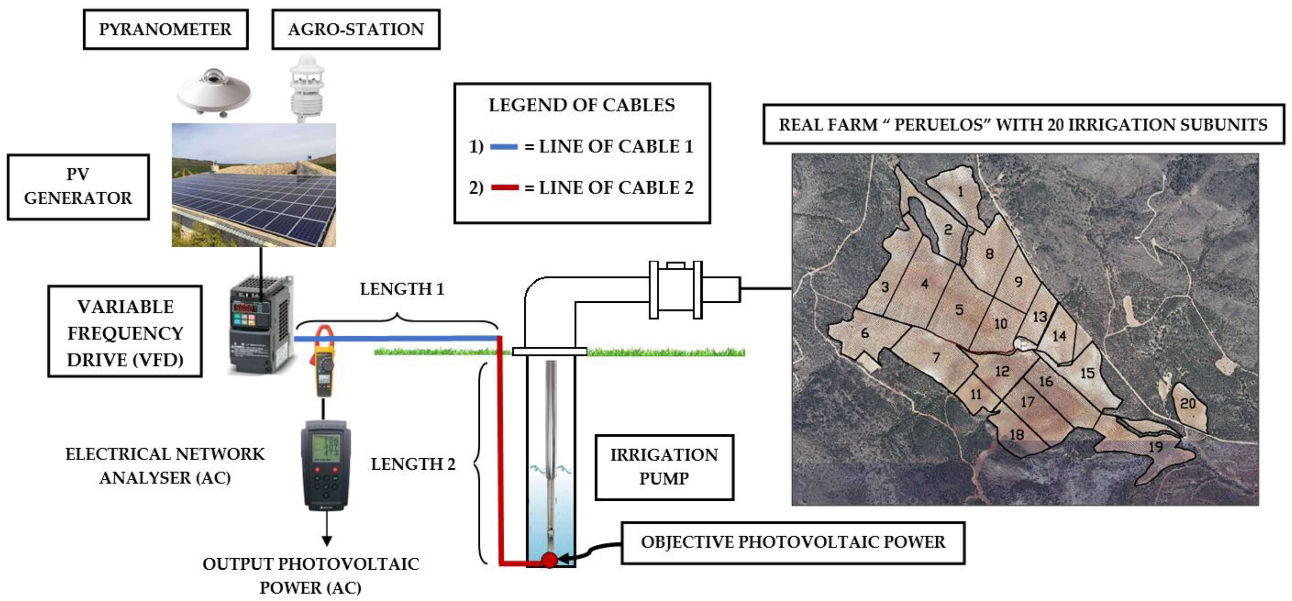
2.1. Case Study and Data Source
2.2. Objective Photovoltaic Power
2.3. Problem Approach
2.4. LSTM Cell
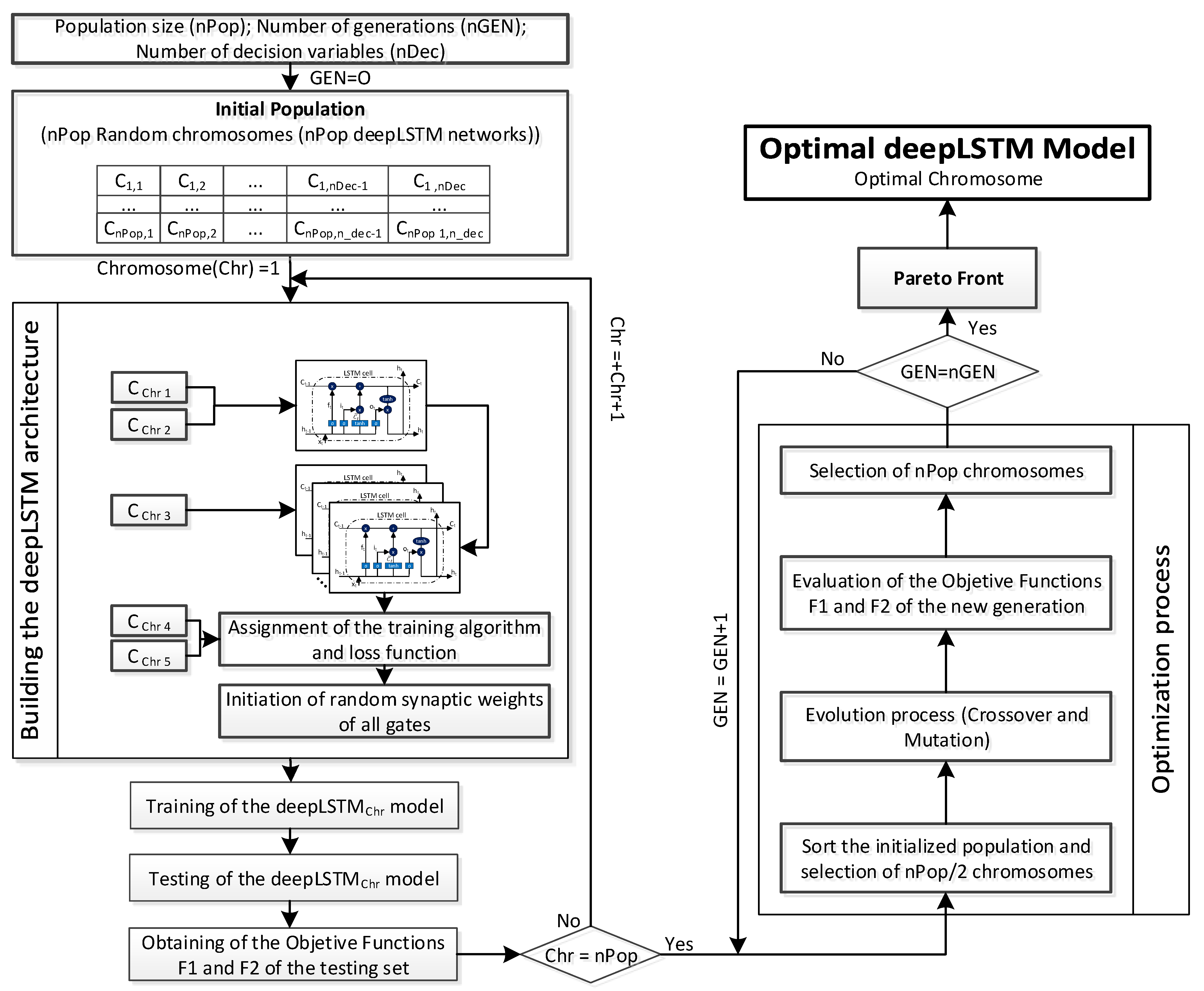
2.5. Building and Optimizing the DeepLSTM Model
3. Results
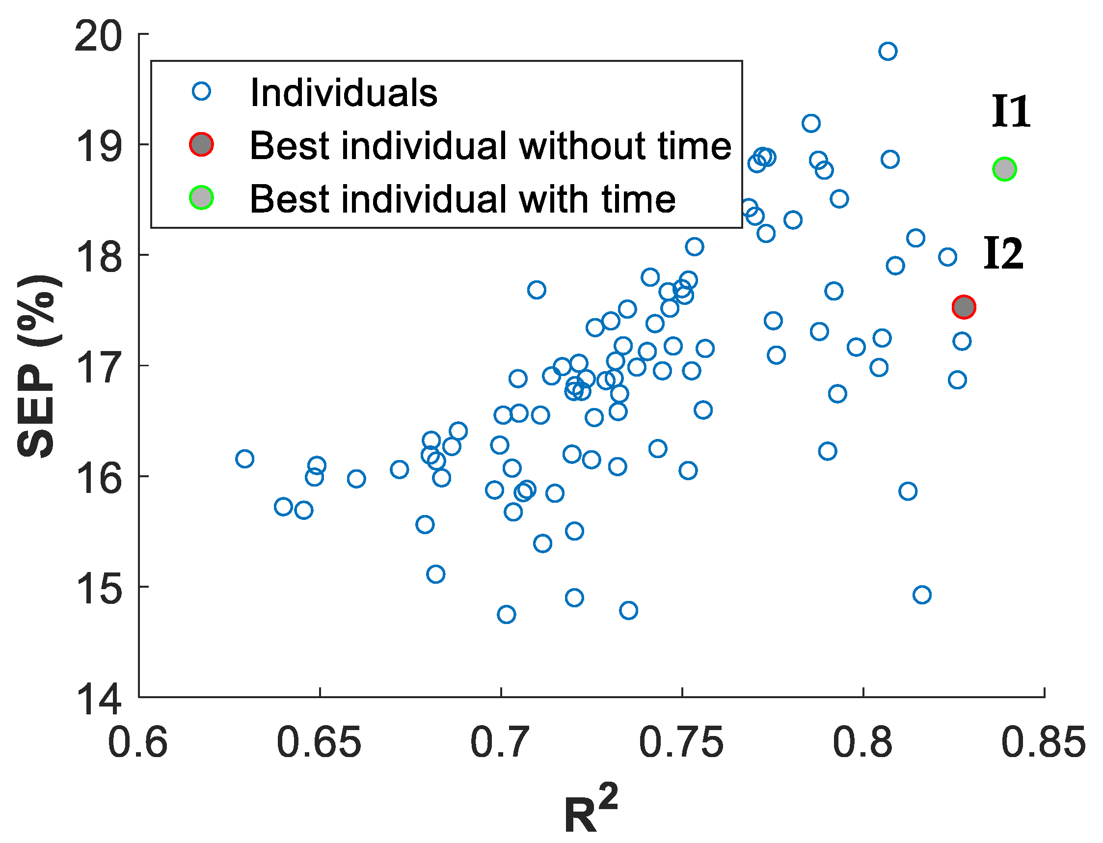
3.1. Evolution of the PREPOSOL Optimization
3.2. Optimal PREPOSOL Model
4. Discussion
5. Conclusions
Author Contributions
Funding
Data Availability Statement
Conflicts of Interest
References
- Yu, J.; Wu, J. The sustainability of agricultural development in China: The agriculture-environment nexus. Sustainability 2018, 10, 1776. [Google Scholar] [CrossRef] [Green Version]
- Garcia, A.V.M.; López-Jiménez, P.A.; Sánchez-Romero, F.J.; Pérez-Sánchez, M. Objectives, keys and results in the water networks to reach the sustainable development goals. Water 2021, 13, 1268. [Google Scholar] [CrossRef]
- Playán, E.; Mateos, L. Modernization and optimization of irrigation systems to increase water productivity. Agric. Water Manag. 2006, 80, 100–116. [Google Scholar] [CrossRef] [Green Version]
- Tarjuelo, J.M.; Rodriguez-Diaz, J.A.; Abadía, R.; Camacho, E.; Rocamora, C.; Moreno, M.A. Efficient water and energy use in irrigation modernization: Lessons from Spanish case studies. Agric. Water Manag. 2015, 162, 67–77. [Google Scholar] [CrossRef]
- Giustolisi, O.; Berardi, L.; Laucelli, D.; Savic, D.; Kapelan, Z. Operational and tactical management of water and energy resources in pressurized systems: Competition at WDSA. J. Water Resour. Plan. Manag. 2016, 142, C4015002. [Google Scholar]
- Raza, F.; Tamoor, M.; Miran, S.; Arif, W.; Kiren, T.; Amjad, W.; Hussain, M.I.; Lee, G.H. The Socio-Economic Impact of Using Photovoltaic (PV) Energy for High-Efficiency Irrigation Systems: A Case Study. Energies 2022, 15, 1198. [Google Scholar] [CrossRef]
- Izquiel, A.; Ballesteros, R.; Tarjuelo, J.M.; Moreno, M.A. Optimal reservoir sizing in on-demand irrigation networks: Application to a collective drip irrigation network in Spain. Biosyst. Eng. 2016, 147, 67–80. [Google Scholar] [CrossRef]
- Guven, G.; Sulun, Y. Pre-service teachers’ knowledge and awareness about renewable energy. Renew. Sustain. Energy Rev. 2017, 80, 663–668. [Google Scholar] [CrossRef]
- Goel, N.; O’Hern, H.; Orosz, M.; Otanicar, T. Annual simulation of photovoltaic retrofits within existing parabolic trough concentrating solar powerplants. Sol. Energy 2020, 211, 600–612. [Google Scholar] [CrossRef]
- Gunderson, I.; Goyette, S.; Gago-Silva, A.; Quiquerez, L.; Lehmann, A. Climate and land-use change impacts on potential solar photovoltaic power generation in the Black Sea region. Environ. Sci. Policy 2015, 46, 70–81. [Google Scholar] [CrossRef]
- Jerez, S.; Tobin, I.; Vautard, R.; Montávez, J.P.; López-Romero, J.M.; Thais, F.; Bartok, B.; Christensen, O.B.; Colette, A.; Déqué, M.; et al. The impact of climate change on photovoltaic power generation in Europe. Nat. Commun. 2015, 6, 10014. [Google Scholar] [CrossRef] [PubMed] [Green Version]
- Vick, B.; Neal, B.; Clark, R.; Holman, A. Water Pumping with AC Motors and Thin-Film Solar Panels. In Proceedings of the Conference, Solar: Including Proceedings of 32nd ASES Annual Conference; American Solar Energy Society: Austin, TX, USA, 2003; pp. 21–26. [Google Scholar]
- Pande, P.C.; Singh, A.K.; Ansari, S.; Vyas, S.K.; Dave, B.K. Design development and testing of a solar PV pump based drip system for orchards. Renew. Energy 2003, 28, 385–396. [Google Scholar] [CrossRef]
- Bouzidi, B. Viability of solar or wind for water pumping systems in the Algerian Sahara regions—Case study Adrar. Renew. Sustain. Energy Rev. 2011, 15, 4436–4442. [Google Scholar] [CrossRef]
- Senol, R. An analysis of solar energy and irrigation systems in Turkey. Energy Policy 2012, 47, 478–486. [Google Scholar] [CrossRef]
- Reca, J.; Torrente, C.; López-Luque, R.; Martínez, J. Feasibility analysis of a standalone direct pumping photovoltaic system for irrigation in Mediterranean greenhouses. Renew. Energy 2016, 85, 1143–1154. [Google Scholar] [CrossRef] [Green Version]
- Calero-Lara, M.; López-Luque, R.; Casares, F.J. Methodological advances in the design of photovoltaic irrigation. Agronomy 2021, 11, 2313. [Google Scholar] [CrossRef]
- Todde, G.; Murgia, L.; Deligios, P.A.; Hogan, R.; Carrelo, I.; Moreira, M.; Pazzona, A.; Ledda, L.; Narvarte, L. Energy and environmental performances of hybrid photovoltaic irrigation systems in Mediterranean intensive and super-intensive olive orchards. Sci. Total Environ. 2019, 651, 2514–2523. [Google Scholar] [CrossRef] [PubMed]
- Ntanos, S.; Skordoulis, M.; Kyriakopoulos, G.; Arabatzis, G.; Chalikias, M.; Galatsidas, S.; Batzios, A.; Katsarou, A. Renewable energy and economic growth: Evidence from European countries. Sustainability 2018, 10, 2626. [Google Scholar] [CrossRef] [Green Version]
- Omri, A.; Nguyen, D.K. On the determinants of renewable energy consumption: International evidence. Energy 2014, 72, 554–560. [Google Scholar] [CrossRef]
- Usman, Z.; Tah, J.; Abanda, H.; Nche, C. A Critical Appraisal of PV-Systems’ Performance. Buildings 2020, 10, 192. [Google Scholar] [CrossRef]
- Antonanzas, J.; Osorio, N.; Escobar, R.; Urraca, R.; Martinez-de-Pison, F.J.; Antonanzas-Torres, F. Review of photovoltaic power forecasting. Sol. Energy 2016, 136, 78–111. [Google Scholar] [CrossRef]
- Sobri, S.; Koohi-Kamali, S.; Rahim, N.A. Solar photovoltaic generation forecasting methods: A review. Energy Convers. Manag. 2018, 156, 459–497. [Google Scholar] [CrossRef]
- Agoua, X.G.; Girard, R.; Kariniotakis, G. Photovoltaic power forecasting: Assessment of the impact of multiple sources of spatio-temporal data on forecast accuracy. Energies 2021, 14, 1432. [Google Scholar] [CrossRef]
- Abiodun, O.I.; Jantan, A.; Omolara, A.E.; Dada, K.V.; Mohamed, N.A.E.; Arshad, H. State-of-the-art in artificial neural network applications: A survey. Heliyon 2018, 4, e00938. [Google Scholar] [CrossRef] [Green Version]
- Elsheikh, A.H.; Sharshir, S.W.; Abd Elaziz, M.; Kabeel, A.E.; Guilan, W.; Haiou, Z. Modeling of solar energy systems using artificial neural network: A comprehensive review. Sol. Energy 2019, 180, 622–639. [Google Scholar] [CrossRef]
- Almonacid, F.; Fernandez, E.F.; Mellit, A.; Kalogirou, S. Review of techniques based on artificial neural networks for the electrical characterization of concentrator photovoltaic technology. Renew. Sustain. Energy Rev. 2017, 75, 938–953. [Google Scholar] [CrossRef]
- Kalani, H.; Sardarabadi, M.; Passandideh-Fard, M. Using artificial neural network models and particle swarm optimization for manner prediction of a photovoltaic thermal nanofluid based collector. Appl. Therm. Eng. 2017, 113, 1170–1177. [Google Scholar] [CrossRef]
- Kamthania, D.; Tiwari, G.N. Performance analysis of a hybrid photovoltaic thermal double pass air collector using ANN. Appl. Sol. Energy (English Transl. Geliotekhnika) 2012, 48, 186–192. [Google Scholar] [CrossRef]
- Ghani, F.; Duke, M.; Carson, J.K. Estimation of photovoltaic conversion efficiency of a building integrated photovoltaic/thermal (BIPV/T) collector array using an artificial neural network. Sol. Energy 2012, 86, 3378–3387. [Google Scholar] [CrossRef]
- Karatepe, E.; Boztepe, M.; Colak, M. Neural network based solar cell model. Energy Convers. Manag. 2006, 47, 1159–1178. [Google Scholar] [CrossRef]
- Mellit, A.; Kalogirou, S.A. MPPT-based artificial intelligence techniques for photovoltaic systems and its implementation into field programmable gate array chips: Review of current status and future perspectives. Energy 2014, 70, 1–21. [Google Scholar] [CrossRef]
- McCandless, T.C.; Haupt, S.E.; Young, G.S. A regime-dependent artificial neural network technique for short-range solar irradiance forecasting. Renew. Energy 2016, 89, 351–359. [Google Scholar] [CrossRef] [Green Version]
- Deb, K.; Pratap, A.; Agarwal, S.; Meyarivan, T. A fast and elitist multiobjective genetic algorithm: NSGA-II. IEEE Trans. Evol. Comput. 2002, 6, 182–197. [Google Scholar] [CrossRef] [Green Version]
- Hochreiter, S.; Urgen Schmidhuber, J. Long Short-Term Memory. Neural Comput. 1997, 9, 17351780. [Google Scholar] [CrossRef] [PubMed]
- Cervera-Gascó, J.; Montero, J.; Moreno, M.A. I-solar, a real-time photovoltaic simulation model for accurate estimation of generated power. Agronomy 2021, 11, 485. [Google Scholar] [CrossRef]
- Cervera-Gascó, J.; Montero, J.; Del Castillo, A.; Tarjuelo, J.M.; Moreno, M.A. EVASOR, an integrated model to manage complex irrigation systems energized by photovoltaic generators. Agronomy 2020, 10, 331. [Google Scholar] [CrossRef] [Green Version]
- Ineichen, P.; Perez, R. A new airmass independent formulation for the linke turbidity coefficient. Sol. Energy 2002, 73, 151–157. [Google Scholar] [CrossRef] [Green Version]
- Perez, R.; Ineichen, P.; Moore, K.; Kmiecik, M.; Chain, C.; George, R.; Vignola, F. A new operational model for satellite-derived irradiances: Description and validation. Sol. Energy 2002, 73, 307–317. [Google Scholar] [CrossRef] [Green Version]
- Lin, Y.; Cunningham III, G.A.; Coggeshall, S. V Input variable identification—fuzzy curves and fuzzy surfaces. Fuzzy Sets Syst. 1996, 82, 65–71. [Google Scholar] [CrossRef]
- Graves, A.; Mohamed, A.R.; Hinton, G. Speech recognition with deep recurrent neural networks. In Proceedings of the 2013 IEEE international conference on acoustics, speech and signal processing, Vancouver, BC, Canada, 26–31 May 2013; pp. 6645–6649. [Google Scholar]
- Chollet, F. Keras Api Documentation 2015. Open Source software library of Neural Networks. Available online: https://keras.io/ (accessed on 1 January 2022).
- Nesterov, Y. A method for solving the convex programming problem with convergence rate O(1/k2). Dokl. Akad. Nauk SSSR 1983, 269, 543–547. [Google Scholar]
- Duchi, J.C.; Bartlett, P.L.; Wainwright, M.J. Randomized smoothing for (parallel) stochastic optimization. Proc. IEEE Conf. Decis. Control 2012, 12, 5442–5444. [Google Scholar]
- Zeiler, M.D. Adadelta: An Adaptive Learning Rate Method. arXiv 2012, arXiv:1212.5701. [Google Scholar]
- Kingma, D.P.; Ba, J.L. Adam: A method for stochastic optimization. In Proceedings of the the 3rd International Conference for Learning Representations, San Diego, CA, USA, 7–9 May 2015. [Google Scholar]
- Dozat, T. Incorporating Nesterov Momentum into Adam. ICLR Work. 2016, 2013–2016. [Google Scholar]
- Ventura, S.; Silva, M.; Pérez-Bendito, D.; Hervás, C. Artificial neural networks for estimation of kinetic analytical parameters. Anal. Chem. 1995, 67, 1521–1525. [Google Scholar] [CrossRef]
- Gómez, J.L.; Martínez, A.O.; Pastoriza, F.T.; Garrido, L.F.; Álvarez, E.G.; García, J.A.O. Photovoltaic power prediction using artificial neural networks and numerical weather data. Sustainability 2020, 12, 10295. [Google Scholar] [CrossRef]
- Zhen, Z.; Wang, Z.; Wang, F.; Mi, Z.; Li, K. Research on a cloud image forecasting approach for solar power forecasting. Energy Procedia 2017, 142, 362–368. [Google Scholar] [CrossRef]
- Sivaneasan, B.; Yu, C.Y.; Goh, K.P. Solar Forecasting using ANN with Fuzzy Logic Pre-processing. Energy Procedia 2017, 143, 727–732. [Google Scholar] [CrossRef]
- Cheddadi, Y.; Cheddadi, H.; Cheddadi, F.; Errahimi, F.; Es-sbai, N. Design and implementation of an intelligent low-cost IoT solution for energy monitoring of photovoltaic stations. SN Appl. Sci. 2020, 2, 1165. [Google Scholar] [CrossRef]
- Mahjoubi, A.; Mechlouch, R.F.; Ben Brahim, A. Data acquisition system for photovoltaic water pumping system in the desert of Tunisia. Procedia Eng. 2012, 33, 268–277. [Google Scholar] [CrossRef] [Green Version]
- AlShafeey, M.; Csáki, C. Evaluating neural network and linear regression photovoltaic power forecasting models based on different input methods. Energy Rep. 2021, 7, 7601–7614. [Google Scholar] [CrossRef]
- Virtuani, A.; Caccivio, M.; Annigoni, E.; Friesen, G.; Chianese, D.; Ballif, C.; Sample, T. 35 years of photovoltaics: Analysis of the TISO-10-kW solar plant, lessons learnt in safety and performance—Part 1. Prog. Photovoltaics Res. Appl. 2019, 27, 328–339. [Google Scholar] [CrossRef]
- Kim, J.; Rabelo, M.; Padi, S.P.; Yousuf, H.; Cho, E.C.; Yi, J. A review of the degradation of photovoltaic modules for life expectancy. Energies 2021, 14, 4278. [Google Scholar] [CrossRef]


| ID | Name | Value Range |
|---|---|---|
| nDec1 | LSTM cell dimension | Integer value between 10 and 600 |
| nDec2 | Activation function of the LSTM cell | Integer value between 1 and 11 [42]: (1) elu; (2) softmax; (3) selu; (4) softplus; (5) softsign; (6) relu; (7) tanh; (8) sigmoid; (9) hard_sigmoid; (10) exponential; (11) linear |
| nDec3 | Number of stacked LSTM cells | Integer value between 1 and 10 |
| nDec4 | Training function | Integer value between 1 and 7: (1) SGD [43]; (2) RMSprop [42]; (3) Adagrad [44]; (4) Adadelta [45]; (5) Adam [46]; (6) Adamax [46]; (7) Nadam [47] |
| nDec5 | Loss function | Integer value between 1 and 6: (1) MAE; (2) MSE; (3) MAPE; (4) MSLE; (5) Huber; (6) LogCosh; |
| Individual Irrigation Strategy | |||
|---|---|---|---|
| Subunit | Power at Pump Inlet (kW) | EU (%) | CVq (%) |
| 3 | 10 | * | * |
| 11 | * | * | |
| 12 | 79.8 | 14.5 | |
| 13 | 83.0 | 12.1 | |
| 14 | 85.0 | 10.6 | |
| 15 | 86.3 | 9.5 | |
| 16 | 87.2 | 8.8 | |
| 17 | 87.9 | 7.9 | |
| 18 | 88.7 | 7.0 | |
| 19 | 90.9 | 5.0 | |
| 20 | 96.7 | 1.9 | |
| 21 | 98.5 | 0.0 | |
| 22 | 98.5 | 0.0 | |
| 23 | 98.5 | 0.0 | |
| 24 | 98.5 | 0.0 | |
| 25 | 98.5 | 0.0 | |
| 26 | 98.5 | 0.0 | |
| 27 | 98.5 | 0.0 | |
| Simultaneous Irrigation Strategy | |||||||
|---|---|---|---|---|---|---|---|
| Subunit | Power at Pump Inlet (kW) | EU (%) | CVq (%) | Subunit | Power at Pump Inlet (kW) | EU (%) | CVq (%) |
| 3 | 10 | * | * | 11 | 10 | * | * |
| 11 | * | * | 11 | * | * | ||
| 12 | * | * | 12 | * | * | ||
| 13 | * | * | 13 | * | * | ||
| 14 | * | * | 14 | * | * | ||
| 15 | * | * | 15 | * | * | ||
| 16 | 79.3 | 15.0 | 16 | 77.6 | 13.9 | ||
| 17 | 82.0 | 12.9 | 17 | 81.5 | 11.4 | ||
| 18 | 83.7 | 11.6 | 18 | 85.2 | 9.2 | ||
| 19 | 85.0 | 10.6 | 19 | 89.0 | 7.1 | ||
| 20 | 85.9 | 9.8 | 20 | 92.4 | 5.3 | ||
| 21 | 86.6 | 9.3 | 21 | 94.9 | 3.6 | ||
| 22 | 87.2 | 8.7 | 22 | 96.7 | 2.3 | ||
| 23 | 87.7 | 8.2 | 23 | 97.7 | 1.3 | ||
| 24 | 88.3 | 7.4 | 24 | 98.4 | 0.3 | ||
| 25 | 89.1 | 6.6 | 25 | 98.5 | 0.0 | ||
| 26 | 91.0 | 4.9 | 26 | 98.5 | 0.0 | ||
| 27 | 95.0 | 2.9 | 27 | 98.5 | 0.0 | ||
| Date | Hour | Predicted Power (kW) | Individual Subunit (3) | Simultaneous Subunits (3–11) |
|---|---|---|---|---|
| 6 July 2018 | 13:20:00 | 23.11 | ✓ | ✓ |
| 6 July 2018 | 13:30:00 | 21.34 | ✓ | ✓ |
| 6 July 2018 | 14:50:00 | 21.27 | ✓ | ✓ |
| 6 July 2018 | 15:00:00 | 20.69 | ✓ | ✓ |
| 6 July 2018 | 15:10:00 | 19.95 | ✓ | ✓ |
| 6 July 2018 | 15:20:00 | 19.47 | ✓ | ✓ |
| 6 July 2018 | 15:30:00 | 18.99 | ✓ | - |
| 6 July 2018 | 15:40:00 | 18.15 | ✓ | - |
| 6 July 2018 | 15:50:00 | 17.25 | ✓ | - |
| 6 July 2018 | 16:00:00 | 16.45 | ✓ | - |
| 6 July 2018 | 16:10:00 | 15.74 | ✓ | - |
| 6 July 2018 | 16:20:00 | 14.60 | ✓ | - |
Publisher’s Note: MDPI stays neutral with regard to jurisdictional claims in published maps and institutional affiliations. |
© 2022 by the authors. Licensee MDPI, Basel, Switzerland. This article is an open access article distributed under the terms and conditions of the Creative Commons Attribution (CC BY) license (https://creativecommons.org/licenses/by/4.0/).
Share and Cite
Cervera-Gascó, J.; Perea, R.G.; Montero, J.; Moreno, M.A. Prediction Model of Photovoltaic Power in Solar Pumping Systems Based on Artificial Intelligence. Agronomy 2022, 12, 693. https://doi.org/10.3390/agronomy12030693
Cervera-Gascó J, Perea RG, Montero J, Moreno MA. Prediction Model of Photovoltaic Power in Solar Pumping Systems Based on Artificial Intelligence. Agronomy. 2022; 12(3):693. https://doi.org/10.3390/agronomy12030693
Chicago/Turabian StyleCervera-Gascó, Jorge, Rafael González Perea, Jesús Montero, and Miguel A. Moreno. 2022. "Prediction Model of Photovoltaic Power in Solar Pumping Systems Based on Artificial Intelligence" Agronomy 12, no. 3: 693. https://doi.org/10.3390/agronomy12030693
APA StyleCervera-Gascó, J., Perea, R. G., Montero, J., & Moreno, M. A. (2022). Prediction Model of Photovoltaic Power in Solar Pumping Systems Based on Artificial Intelligence. Agronomy, 12(3), 693. https://doi.org/10.3390/agronomy12030693