Abstract
This study attempts to utilize newly developed machine learning techniques in order to develop a general prediction algorithm for agricultural soils in Saudi Arabia, specifically in the Taif region. Energy dispersive X-ray fluorescence (EDXRF) measurements were used to develop national predictive models that predict the concentrations of 14 micronutrients in soils of Taif rose farms, for providing high-quality data comparable to conventional methods. Machine learning algorithms used in this study included the simple linear model, the multivariate linear regression (MLR); and two nonlinear models, the random forest (RF) and multivariate adaptive regression splines (MARS). Our study proposes a machine learning (ML) strategy for predicting fertility parameters more accurately in agricultural soils using 10 farms of the Taif rose (Rosa damascena) in Taif, Saudi Arabia as a case study. Results demonstrated that MARS provides higher prediction performance when the number of explanatory variables is small, while RF is superior when the number of variables is large. On the other hand, the MLR is recommended as a moderate method for predicting multivariate variables. The study showed that multivariate models can be used to overwhelm the drawbacks of the EDXRF device, such as high detection limits and an element that cannot be directly measured.
1. Introduction
One of the most important crops in the floriculture industry [1] is roses, which are used as cut flowers, potted plants, and garden plants [2] and have been used in the perfumery, cosmetics, and food industries for several years [3,4]. Roses belong to the genus Rosa which comprises over 100 widely distributed species in Asia, the Middle East, Europe, and North America [5]. Out of them, only some species have been used for essential oil manufacturing, among which R. damascena is superior in the production of high-value essential oil [6]. The name of the species (damascene) is derived from Damascus, Syria, where it originally emerged as a wild plant. Currently, it is cultivated in different countries around the world [7].
In Saudi Arabia, Rosa damascena has a prolonged history in the Western province, particularly in the Taif region, in which a high-quality rose essential oil is produced, and traditional culture and strong financial productivity have been established over time and created a central area in the international agribusiness [8]. The global demand for high-grade natural R. damascena essential oil has been growing for use in various industries. In order to meet the growing demand for rose oil, there is an urgent need to figure out how ecological and agronomical factors directly influence the productivity of R. damascena essential oil. In many areas of Saudi Arabia, high-quality water supply has become progressively restricted, because of the decrease in rains and the increase in the salinity of groundwaters which contain high levels of soluble salts [9]. Although R. damascena is adapted to a wide scale of environmental conditions, the content, relative compositions, and quality of oil are strongly influenced by ecological and agronomical practices [8]. For this reason, studying rose ecology is a central issue to ensure sustainable productivity of the essential oil of roses and to improve its production across different farms.
Micronutrient and toxic element concentration mapping in agricultural soil is essential but is not widely undertaken, even though this sort of information might be useful in precision agriculture, where the optimal management in space and time is the main goal [10]. For example, copper (Cu), Ferrous (Fe), and zinc (Zn) are important elements for crop production due to their vital roles in photosynthesis, respiration, and other plant functions [11,12]. However, high concentrations can be toxic for crops e.g., the excessive concentration of Cu can cause deformity of root systems [12]. Thus, it is necessary to detect both low and high levels. Moreover, cadmium (Cd) is also toxic to the consumers of crop products above certain threshold concentrations [11]. Hence, it can be helpful to map micronutrients at the field scale to address shortcomings and toxicities; and to improve crop quality. In general, the plant growth and flower yield of Taif roses are known to be reduced as a result of an imbalance of micronutrients [8]. It has been reported that these essential elements play a significant role in the growth and development of roses [13], a fact that requires the availability of these microelements in suitable amounts in the soil.
Globally, innovative technologies play a vital role in all sectors, particularly agriculture. However, traditional methods are still being used in agricultural practices in developing countries. Detecting nutrient deficiency in agricultural soils remains difficult for farmers, as using conventional methods to examine nutrient deficiency consumes more time, labour, and cost. Nutrient deficiencies are normally assayed via agricultural laboratories and experienced people (farmers). Hence, manual predictions of nutritional deficiencies may be inaccurate due to several environmental conditions. To our knowledge, there are no public field-scale maps of microelements in farms of Taif roses.
To derive accurate maps of elemental concentrations in soil, many soil samples need to be analyzed. The conventional method requires element extraction with acids followed by analysis using the inductively coupled plasma (ICP) technique. However, this type of wet chemical analysis can be expensive, time-consuming, and destructive for samples [14]. On the other hand, X-ray fluorescence (XRF) technology is increasingly being developed as an alternative option, as it is an inexpensive, fast, and non-destructive method for analyzing element concentrations in soil samples [15]. This technique is more appropriate where high sampling density is needed (e.g., mapping and geostatistics) [16]. Machine Learning (ML) algorithms have been used to evaluate soil quality parameters coupled with non-destructive methodologies [17]. Among spectroscopic analytical methodologies, energy dispersive X-ray fluorescence (EDXRF) is one of the fastest, most eco-friendly, and least costly methods compared to conventional methods. However, some EDXRF spectra still require more effective methods capable of offering precise outcomes. Energy Dispersive X-ray Fluorescence (EDXRF) spectra were used as input information to improve the prediction of soil analysis using machine learning algorithms. Combined with a simple soil preparation method, this strategy can provide high-quality data comparable to those obtained with a conventional method for evaluating certain elements in the soil. The linear regression (LR) model has been used to evaluate the accuracy of XRF measurements [18,19,20]. Caporale et al. [21] have defined metal-based linear models that predict laboratory concentrations from XRF measurements for agricultural and industrial sites [21,22].
Generally, previous studies showed that more advanced modeling techniques produced better results compared with simpler approaches. Sirsat et al. [23] compared 76 different algorithms, in which ensembles of extremely randomized regression trees proved the most effective in predicting soil fertility indices. Several studies have found ML methods to be more efficient than simpler approaches (principal component regression, partial least squares regression, etc.). Concerning the relationship between performance and model usage, we observed that some simpler methods such as MLR are very popular even though they perform poorly compared to more advanced approaches. This is expected for statistical models since they have a long tradition in science.
Several studies have reviewed the utilization of ML techniques in the context of soil sciences in many countries around the world but are mostly concentrated in developed countries [24,25,26]. A wide variety of machine learning models are available, and over a hundred different variants have been applied in soil sciences [27,28,29,30,31]. While almost all of the models are being used more often, it is possible to observe a decrease in the use of some models, such as support vector machines (SVM), multivariate adaptive regression spline (MARS), and CART, as opposed to more advanced alternatives, such as random forest (RF). The adoption of the latter has accelerated growth, and it has been used in a diversity of topics, including mapping and spectroscopy. There is also an emergence of deep learning methods, which at this point have been used in only a handful of publications related to mapping and spectroscopy. Several studies have concentrated on modeling, particularly mapping, continuous soil properties [32,33,34,35].
Fathololoumi et al. [36] conducted research on improved digital soil mapping in Iran by combining multitemporal remotely sensed satellite data with random forest (RF) and cubist models. Their findings indicated that the cubist model performed better when modeling soil nutrients, while Forkuor et al. [37] suggested the RF model performed better. In addition, Emadi et al. [38] reported the deep neural network (DNN) model to be a superior method of predicting and mapping soil organic carbon using MLA [39]. The study by Bian et al. [40] combines multiple stepwise regression (MSR) analysis, boosted regression trees (BRT) modeling, and boosted regression trees hybrid residuals kriging (BRTRK) to model soil nutrients. Similarly, Taghizadeh-Mehrjardi et al. [41] used the artificial neural network (ANN), support vector regression (SVR), k-nearest neighbor (kNN), random forest (RF), regression tree model (RT), and genetic programming (GP) to predict soil nutrients.
A key objective of this research is to utilize the recently improved machine learning techniques to develop a general prediction performance for agricultural soils in Saudi Arabia, specifically the area of Taif. The specific aims were to: First, use XRF measurements to develop national models for predicting concentrations of 14 micronutrients in agricultural soils of Taif roses farms; the methodology is based on the UniQuant standardless method along with the free-powder technique, which is highly effective when analyzing samples for which no standard is available. UniQuant unifies all types of samples into one single analytical technique, and it is the only method that provides an in-depth analysis of all types of samples. Second, validate the models at the farm scale by using cross-validation. Third, compare the performance of three model types: multiple linear regression (MLR), multivariate adaptive regression splines (MARS), and random forest regression (RF).
2. Materials and Methods
2.1. Study Area
The study area (Figure 1) is located in Taif City in Makkah Province, Saudi Arabia which is located on the eastern slopes of the Al-Sarawat Mountains at 1879 m (6165 ft) elevation (from 21°21′39.21″ N 40°15′47.69″ E to 21°21′24.08″ N 40°14′21.93″ E). The foothills and highland slopes are created mainly of resistant, coarse, pink granite, mixed with grey diorite and granodiorite. The climate is arid with 181 mm 30-year average annual rainfall. The rainy season is between April and November, and the mean annual temperature is 22.8 °C, with the coldest mean temperatures (15 °C) in January and the warmest (29 °C) in July [42]. The rainfall in the region is erratic and irregular, the high precipitation occurs in May (30.6 mm/day) and in November (21.5 mm/day), however, precipitation is scarce throughout the other months. The mean monthly relative humidity ranges from 23% in June to 60% in January. The area is located within the southern part of the region. Cropland soil texture ranges from sandy to sandy loam generally dominating in the south and southwestern agricultural areas [43]. It is an important rose supply base for the kingdom of Saudi Arabia. Located within the Taif area is an agricultural area that is one of the best-known in Saudi Arabia.
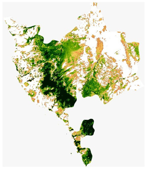
Figure 1.
Map of Makkah province demonstrating the study area, obtained from MODIS satellite Image Collection via Google Earth using bespoke python code.
2.2. Soil Sampling
Soil samples were collected from cultivated rose farms in 2021 at two different randomly chosen sites in Taif in the mountains of Shafa and Hada. The mountains are located Southwest and Northwest of Taif City, respectively. The locations of the sampling sites were determined by a global position system (GPS) device. Soil samples from 10 farms (n = 2000, ~200 from several fields per farm) were used for validation at the farm scale. The ten farms were originally selected to represent a wide range of chemical and physical characteristics and different geologies. Each soil sample consisted of a mixture of four subsamples collected around the site. After removing the surface layer, the soil was collected at a depth of 20 cm avoiding the open slit. Approximately 1000 g of soil was collected with a wooden shovel at each site and stored in a clean self-sealing polyethylene bag. After collection, the soil samples were air-dried, homogenized, and sieved (<2 mm) to remove the coarse fraction, then samples were transported to the laboratory for further analysis
2.3. XRF Measurements
XRF analysis was carried out with soil samples that had been air-dried in the open air for seven days to reduce moisture content below 20%. This is because samples above 20% moisture content may interfere with the XRF analysis and may alter the soil matrix for which the XRF spectrometer has been calibrated [44,45], with respect to solid (powdered) samples. For this purpose, we prepared the samples for drying by breaking them down into aggregates and spreading them evenly on polyethylene sheets or plywood trays in the open air, while ensuring that there were no cross-contaminations or contamination from any external source(s). To reduce the effect of the soil matrix, the samples were homogenized and sieved to a particle size of about 75 μm with Retsch aluminum test sieves and a vibratory shaker. XRF spectrometers only analyze a sample’s surface layer, which must be representative of the entire sample, so each soil sample was carefully and uniformly ground into pellets with smooth surfaces of equal density, as described by Kodom et al. [44]. By milling or pulverizing the loose powdered samples (75 μm), the particle size was further reduced to 60 μm and lower.
XRF analysis of soil samples was performed using the UniQuant standardless method and the free-powder technique on an Energy-dispersive X-ray fluorescence spectrometer, Thermo Fisher Scientific, Quant’ X. UniQuant is a complete application for standardless semiquantitative to quantitative XRF analysis conducted utilizing an X-ray sequential spectrometer. The ground sample was placed in a preassembled sample plastic cup (40 mm diameter, 38.4 mm height) and covered with a polypropylene support thin film 3–6 µm thickness (Chemplex industries Inco, Palm City, FL, USA). The samples were irradiated in triplicate for 300 s under vacuum using an Rh X-ray tube at 15 kV (Na to Sc) and 50 kV. The current was automatically adjusted (maximum of 1 mA). A 10 mm collimator and a Si (Li) detector were used, and then it was cooled with liquid nitrogen for detection. Poor handling of the samples could seriously influence the results of the analysis due to the sensitivity of the spectrometer, which was sensitive enough to detect fingerprints on the pellet’s surface layer [44,45,46].
The XRF Quant’ X analyzer was used to analyze Si, Al, Fe, Ti, Cl, Mn, Sr, Ba, Zr, Zn, Cu, Cr, Y, and Ni in representative fractions of the soil samples in accordance with the EPA method [46]. For the ideal “mining” procedure under vacuum, limits of detection (LODs) were within the range of 2 mg kg−1 (e.g., Ni and Cu) and 60 mg kg−1 (e.g., Cl).
2.4. Modeling
This section is devoted to present the approaches and techniques used in the development and assessment of the three models used in this study, namely: Multiple linear regression (MLR), random forest (RF), and multivariate adaptive regression spline (MARS). In Section 2.4.1, an overview of the mathematical background supporting these models is provided, as well as the symbols and notations used to develop them. In Section 2.4.2, a description is given of the implementation’s parameters and validation methods.
2.4.1. Overview of MLR, RF, and MARS
Modeling the concentrations of soil microelements in the Taif rose Farms is carried out here using the following three machine learning algorithms (i) Multiple linear regression (MLR), (ii) random forest (RF), and (iii) multivariate adaptive regression spline (MARS). The key reason for restricting our attention to these three algorithms is the vast and diverse assumptions and solving techniques they have. The MLR assumes the relations between the dependent and explanatory variables can be represented as a collection of lines whose optimal parameter spaces can be determined by minimizing the distance between the algebraic sum of these lines and the dependent’s ground truth. In contrast, both RF and MARS relax the MLR’s linear assumptions, the RF is an ensemble of several decision trees that works collaboratively to figure out the relations between the variables under investigation without imposing a prior assumption about the type of these relations. Hastie et al. [47] has provided a more detailed description of MLR, RF, and MARS.
In order to describe the aforementioned model formally, let be a tabular dataset comprising the readings of the samples collected from the 10 Taif rose farms. The dimension of is given as where is the number of measured microelements, i.e., 14 in this study, and is the number of readings. For the purpose of processing this dataset, the is divided into 14 vectors numbered from 1 to 14 each of which contains the readings of specific microelement, hence , is used to refer the readings of the ith microelements.
In the proposed MLR model, each microelement vector, i.e., is used as the dependent variable whereas the remaining 13 vectors, i.e., are used as explanatory variables. Therefore, the main objective of the MLR can be described as finding the coefficients for each instance of that facilitates computing as a sum of , i.e.,
where is the projected values generated from the model, is the y-intercept, i.e., the value of when all the values of all s are set to 0 and is the vector of errors values that yields from computing in terms of [48].
The proposed random forest model is based on a bagging approach, in which vectors other than the independent variable are segregated randomly and converted to several sub-vectors [49]. Thereafter, each sub-vector is fed into a dedicated regression model (i.e., a decision tree model) created by the random forest engine. This engine then trains each model individually, collects the votes from each model and aggregates them, for this reason most references refer to the random forest as a bootstrap aggregation technique. To describe this operation mathematically, let us assume that the vector of the th microelement readings, i.e., is divided into sub-vectors each of which is trained with a model whose output is denoted by , where refers to the cardinality of (the number of sub-vectors) then the output of the random forest model, , can be written as:
where is the sub-vector of that is used by the model to generate and is the hyperparameters spaces used by that model to generate the results. This hyperparameters space comprises those criteria upon which the models are built, such as the number of the models (i.e., decision trees), their depth, and the number of the explanatory vectors. It is worthy to note that the highly parametric approach of the random forest makes it more suitable for treating nonlinear problems better than MLR; however, this comes at the expense of increasing the computational power. Particularly, adding more models can make the model able to differentiate more combinations of the sub-vectors, which in turn can boost prediction performance, however such operations entail substantial overhead. Finally, the proposed MARS utilized the divide and conquer techniques to group the inputted dataset, i.e., and their associated features, i.e., , into several piecewise linear parts (i.e., splines) each of which has its own gradients. The MARS thereupon endeavors to attach these splines firmly to generate the best possible representation of in terms of . In mathematical parlance, the predicted values of can be written as:
where , dubbed basis function, is the transformation that is used to connect the splines and is the fitting error. MARS traditionally uses the stepwise searching technique to specify the number of splines’ joint points, which are referred to as knots. The technique consists of two phases: forward and backward, with the forward phase defining the knot locations randomly, as well as the backward phase adjusting the knot numbers and locations according to the fitting errors [50]. As a result of alternate forward and backward phases, the MARS is able to reduce errors and hence provide the best possible representation for the independent variable.
2.4.2. Model Implementation and Validation
All the programming and modeling efforts were carried out over a single machine running a Ubuntu operating system on the 11th generation Intel core processor, with a speed of 5.3 GHz with 8 core/16 threads. The machine used 62 GB of memory and a GeoForce RTX 2060 graphical processor unit. Python version 3.10.2 with Scikit-learn package [51] was used to model the MLR and RF whereas the Py-earth package [52] was used to implement MARS. The default values of the RF and MARS as specified in the respective packages were used to treat the datasets, this includes using additive MARS approaches and the number of initial instances of trees in RF (which is 100). All the outcomes of the proposed models were assessed using standard statistical measurements.
It should be noted that, despite the differences between the three modeling techniques evaluated in this study, Equations (1)–(3) show that the predicted value (the concentration of a specific microelement) of each model depends primarily on the explanatory variables (the concentration of one or more microelements). This, in turn, raises the question of which explanatory variables may be effective for each model to yield accurate predicted values. Motivated by the need to address this question, we employed the combination theory [53] to generate all possible arrangements that can be used as explanatory variables for each microelement. This approach gave 8191 possible arrangements for each microelement and in total 114,674 possible arrangements for all microelements. A dedicated MLR model was constructed for each one of the 114,674 arrangements; thereupon new models based on the RF and MARS were used instead of the MLR. Hence the total number of models used in this study was models or 344,022. Figure 2 illustrates our proposed approach, in which all possible arrangements to compute the Si microelement were generated using MLR. Figure 2a illustrates how the other 13 microelements (all of the elements other than Si) were used independently as explanatory variables, this yields a models where denotes the combination operator. Figure 2b shows that the same 13 microelements (i.e., all the microelements except Si) were used as explanatory variables to predict Si. However, instead of feeding each variable at a time, they were grouped in pairs, i.e., using the concentrations of Al and Fe together to predict the concentration of Si, and then usage of Al with Ti to predict the concentration of Si, and so on until we had covered all possible combinations, this yielded possible combinations. Figure 2c illustrates that the same technique used in Figure 2a,b was employed, except that the 13 microelements were grouped in a tuple of 3 instead of 2 i.e., . This procedure continued until the model used all 13 microelements together for Si prediction (Figure 2d,e). Figure 3 shows how the outputs from each model were constructed.
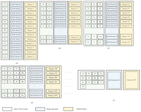
Figure 2.
High level abstract for the proposed approach, in which all possible arrangements, to predict the Si microelement are generated, using MLR. (a) each microelement except Si has been used individually as explanatory variable, (b) two microelements except Si have been used as explanatory variable, (c) three microelements except Si have been used as explanatory variable, (d) four microelements except Si have been used as explanatory variable, (e) all microelements except Si have been used as explanatory variable.
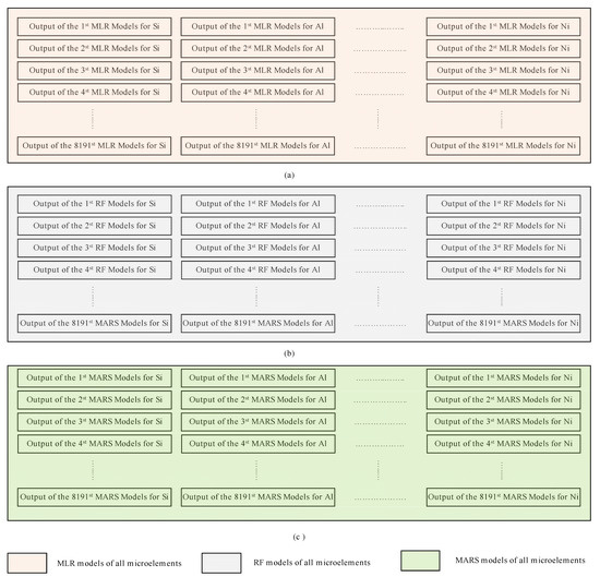
Figure 3.
The method used to construct the outputs from the three different models used in this study (MLR, RF, and MARS) (a) models generated using MLR, (b) models generated using RF, (c) models generated using MARS.
For comprehensive evaluation of the performance of the modeling techniques, namely MLR, RF, and MARS, the 10-fold cross-validation scheme was employed. In this scheme, the dataset was randomly divided into 10 even-sized subsets, with nine of the ten subsets being used in the training of the model, while the tenth was used in the test phase. This procedure was repeated 10 times in order to permit each subset to be used in the test phase. An advantage of this scheme is that it enables the testing of the prediction accuracy of the model from different perspectives without being influenced by the distributions within the dataset. This provides more robust estimations for the model’s performance. Figure 4 shows an abstract of this operation at a high level.
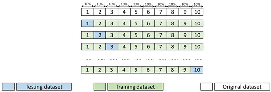
Figure 4.
Evaluation of the modeling techniques performance of MLR, RF, and MARS, using the 10-fold cross validation scheme.
3. Results and Discussion
3.1. Measurements of EDXRF of the Farm Dataset
A description of the EDXRF-analyzed elemental concentrations for the selected farms is presented in Table 1. As there are no national reference values available, we had to use international reference values for element concentrations in soils as calibration and cross-validation data (Table 1). Interestingly, the EDXRF generated dataset is within the range of previously recorded values, which makes it possible to utilize it to validate the models. It is worth noting that the selected farms (L1-L10) differed in their frequency distributions of micronutrient concentrations. For instance, L10 had higher Ba and Zr concentrations, while L6 had higher Zn and Cr concentrations (Table 1). However, regardless of the range of reference measurements, the average values of the measured concentrations showed that the farm dataset revealed a greater Fe and Ti concentration than the reference values. For example, compared to 2.6% and 0.29% of Fe and Ti all the studied farms contained 3.9–6.78% and 0.43–0.85%, respectively (Table 1). Similarly, eight samples in the farm dataset had Zn and Si concentrations above 0.006% and 31%, respectively.

Table 1.
Results of EDXRF analysis of micronutrients in samples of agricultural soils collected from the study area according to Koom et al. [44]. The data represent the mean value of element concentration (mg kg−1). As there is no common LOD for an element, measured values below this limit were denoted “not a number” (NaN) value. (E) denotes element. The farms included in this study were designated from L1-L10. Reference element concentrations are based on Shacklette, Hansford [54], and Al-Mamoori et al. [55].
3.2. Performance Metrics
The following metrics were used to measure the performance of the models: mean absolute error (), mean absolute percentage error (), mean squared error (), and mean square percentage error (), relative absolute error (), relative squared error (), and R-squared ().
The measures the average of the Manhattan distance between each ground truth value and its corresponding predicted value generated by the model. In order to describe in the context of this study, let be the th elements of the ground truth vector that accommodates all the readings of the th microelements taken from the Taif rose farms, i.e., and is the predicted value of , then can be given as [56]:
The value of the can be interpreted intuitively as the extent to which the predicted values generated from the model differ from the ground truth values on average; hence the closer to zero the better prediction performance and vice versa. While the is regarded as one of the most significant metrics that can be used to quantify the overall performance of a model, since it measures the absolute error, it makes its readings unbounded; thus, other metrics have appeared in the open literature. The mean absolute percentage error () metric analyses predictive errors in the same manner as . However, normalizes the calculated error in relation to the ground truth readings and multiplies the result by 100 to lessen the sensitivity of the model to a deviation from the true value. Formally, can be written as:
readings are interpreted similarly to readings; for example, higher values mean that the predicted values generated from the model are large in contrast to the ground truth values, and vice versa. Despite the advantages of and , they are unable to account for certain types of errors, such as outliers, inliers, non-linear correlations, or uplift due to their use of Manhattan distance to measure error. Motivated by the need to develop a meaningful metric to evaluate such errors, the mean squared error () and mean square percentage error () have been introduced. MSE and MSPE can be described mathematically as [57]:
When comparing Equation (4) with (6) and (5) with (7), it can be seen that there is a significant difference between them, as and use the Euclidean distance in the lieu of the Manhattan distance. As a result of the Euclidean distance, the larger errors have a greater contribution to the and values, which in turn allows them to overcome the shortcomings of and
Even though the above performance metrics can be used to quantify prediction accuracy, comparing two models requires more sophisticated measures that are more directly proportional to the weights associated with each prediction error. Therefore, a new family of performance metrics have been devised to provide more robust measures, such as relative absolute error () and relative squared error (). The and can be given as [58]:
where is the arithmetic mean of the vector . It is noteworthy that the square of the difference between the ground truth reading and the arithmetic mean reading should be used in the denominator of the model rather than the cardinality of the as in and which allows and to compare the model’s performance with another simple model that uses the arithmetic mean as predictor. This means the outputs of the and are real valued numbers ranging from zero to one, where zero implies that the model is performing optimally, and zero implies that the model is performing poorly.
The last performance metric considered in this study is the R-Squared () which can be defined as [59]:
is simply the ratio between the total variation presented by the predicted values generated from the model with respect to the arithmetic mean of the ground truth values and the total variation presented by the ground truth values themselves with respect to their arithmetic mean. The output of the metric is a real value number bounded over the range [0,1] and cbe interpreted in a similar manner as the output of and
3.3. Modeling
Fundamentally, RF segregates the space of the considered datasets into a set of sub-datasets and then feeds each of which into several decision trees whose main responsibility is to figure out the relations between the given sub-datasets and to conduct the prediction processes accordingly. RF then averages all the outcomes of these trees to generate the single results. Although MARS is like RF in that both are nonparametric algorithms, MARS differs substantially in the way that it is used to treat the dataset and is employed to define the relations between variables. Basically, MARS assumes that the considered dataset can be represented as a family of polynomials that are valid within a spectrum of the explanatory variables; accordingly, MARS assesses the cut-points of these polynomials to generate a system of the piecewise linear regression model of candidate features. Once MARS allocates the vicinities of the near-optimal solutions of the model, it applies the hinge function to alternate the computations of the generated system of equation between forward and backward cycles with the aim of expediting the approach to the optimal representation region and to reduce overfitting and model complexity.
To predict the concentration of an element based on the concentrations of other elements the correlation coefficient for the raw data was computed (Figure 5) while the MLR was applied to show the optimal values for each element (Table 2). The correlation matrix of the microelement’s readings obtained from the farms as given in Figure 2 demonstrates that out of the 14 microelements, Zr had the highest correlation readings; more specifically, Zr was correlated positively with Ba and Y at values of +0.8 and +0.73, respectively, and negatively with Fe and Si at values of −0.72 and −0.69, respectively. On the other hand, it was noticed that the lowest correlation readings were due to Cl elements, as it correlated with Si and Al by values of 0.00157 and −0.00366, respectively. The diagonal of this matrix is the histogram of the microelements, and the lower section is the scatter plots of the pairs of elements.
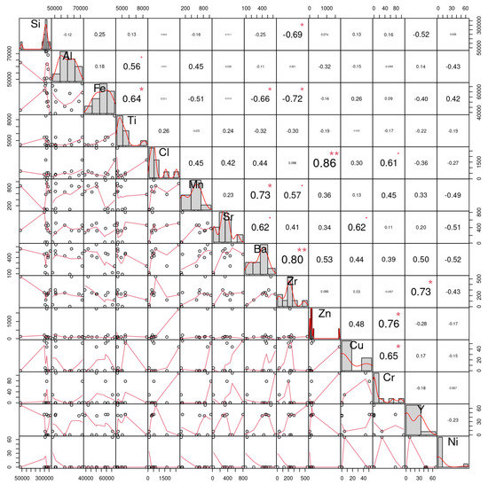
Figure 5.
The correlation matrix of the 14 microelement’s readings obtained from the studied Taif rose farms for prediction of the concentration of an element based on the concentrations of other elements. the signal asterisk (*) indicate the correlation is significant at the 0.05 level and double asterisk (**) indicate indicates the correlation is significant at the 0.01 level.
Table 2.
The coefficients of microelements that generate the optimal prediction performance for each element.
Figure 6 illustrates the boxplot of the 14 microelements considered in this study. A boxplot is amongst the standardized tools that can be used to exhibit statistical information of a dataset using five values: minimum, first quartile, median, third quartile, and the maximum readings of the dataset. Hence, the short boxplot as was the case for Ni, Zn, Si, and Cl demonstrate that the readings of these elements across the Taif rose fields were of high agreement with each other, i.e., the dispersion of these readings were slight and hence all the aforementioned statistical measurements occurred with a small range. On the other hand, the long boxplots like those of the Al, Mn, Cu, and Y datasets indicated that these microelement values were spread out over a large range. Interestingly, boxplots can also be used to give an indication of the density of the readings within a given range. It can be seen, for instance, that most of the Cu readings were concentrated within the above Q2 intervals whereas the opposite case can be seen for Mn.
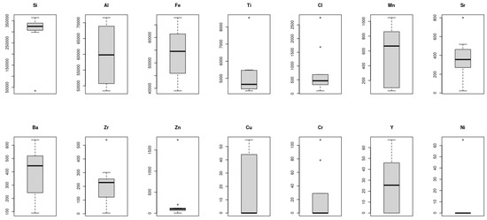
Figure 6.
Boxplot of the 14 microelements considered in this study, which was used to exhibit statistical information of a dataset. The short boxplots (e.g., Ni, Zn, Si, and Cl) indicate high correlations among the readings of the elements and very small dispersion. The long boxplots (e.g., Al, Mn, Cu, and Y) datasets indicate that these microelements’ values are spread out over a large range.
3.4. Validation
Assessment for the validity of our readings was conducted by comparing them with those that have been recorded in previous reports, e.g., [54,55]. The results of this assessment are given in Figure 6 where the green area is used to indicate the range of values and the blue columns signify the average values of the considered element’s datasets. As indicated from these results, some values are shown to fall near the average (e.g., Si, Ba, and Ni) whereas others fall on the boundaries (e.g., Cl, Cr, and Cu). However, all the collected readings fell within the reported range which provided a face validation for the methods by which the raw data was collected and analysed (Figure 7).
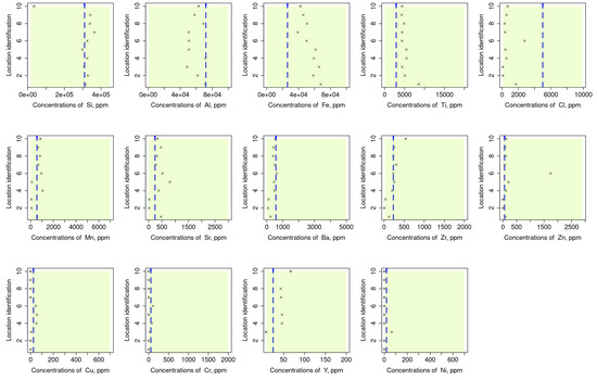
Figure 7.
Comparison of the measurements in the studied area to assess the validity of our readings concerning reference values that have been recorded in previous reports, e.g., [54,55]. Green area indicates the range of values, and the blue columns signify the average values of the considered element’s datasets. Some values are shown to fall near the average (e.g., Si, Ba, and Ni) whereas the others fall on the boundaries (e.g., Cl, Cr, and Cu).
3.5. Outcomes of the MLR, RF, and MARS
We investigated all combinations of these variables since the performance of the MLR model depends largely on the formula used to reveal latent relationships between the dependent and explanatory variables. Hence, we employed the permutation approach to construct 196 MLR models, each describing possible relationships between the dependent variables and other explanatory variables that led to the best results. Figure 8 shows the models constructed to reveal the relation between Si as an independent element and other elements.
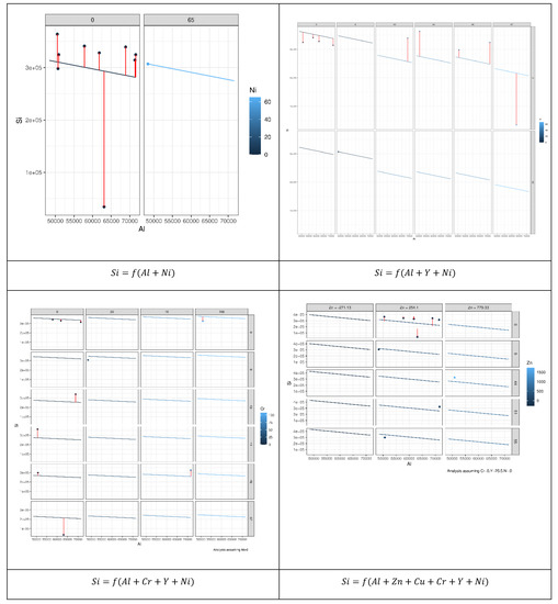
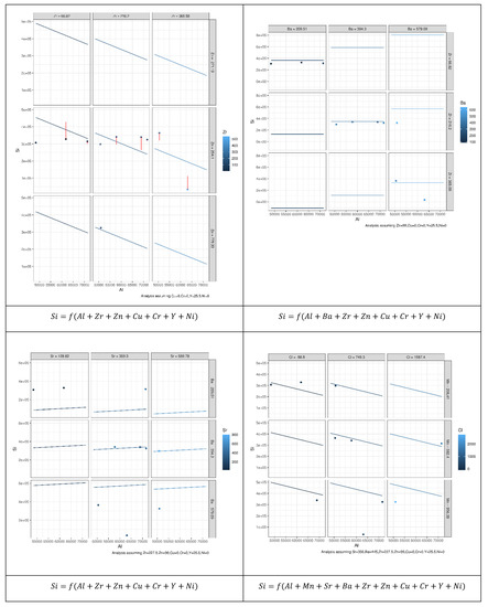
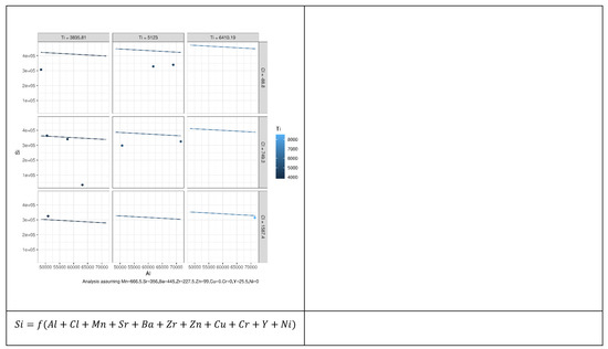
Figure 8.
Prediction error of 196 MLR models constructed to reveal the relation between Si as an independent element and other elements based on the permutation approach. Each model describes possible relationships between the dependent variables and other explanatory variables that led to the best results.
As can be seen from Figure 9, not all explanatory elements have the same contribution to the prediction of Si and an increase in the number of explanatory variables can improve the prediction performance. Comparing the case where both Al and Ni were used to predict Si with the case where Al, Y, and Ni were used showed that the error bars (vertical lines) of the latter case were shorter than the former. Table 2 presents the coefficients of microelements that generated the optimal prediction performance for each element. The same permutation technique used to obtain the results of MLR was applied to obtain the results of the random forest (RF). According to Figure 8, we can see that different elements had different error prediction characteristics, from which one may be able to determine the best number of trees to use. For instance, the optimal number of trees for Si was approximately 50, whereas the optimal number of trees for Al was approximately 30. Table 3 shows the maximum values of the number of trees and their error readings of RF.
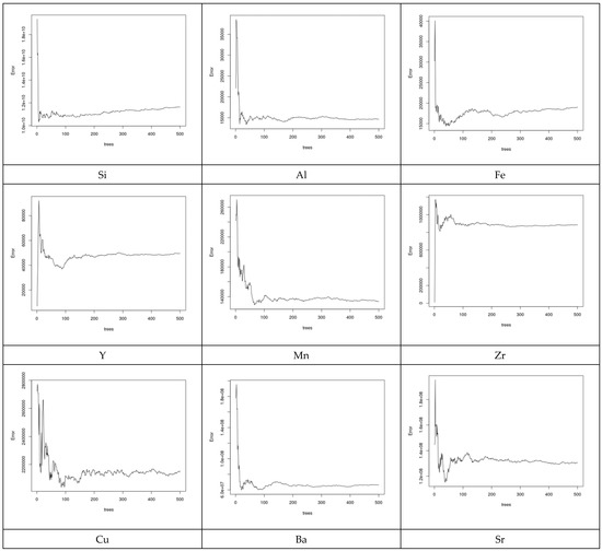
Figure 9.
Prediction error of the RF models for some selected elements. Different elements have different error prediction characteristics to determine the best number of trees to use.
Table 3.
Maximum values of the number of trees and their error readings of RF.
Considering the MARS models, a sample of four prediction performances is shown in Figure 10, including the cumulative distribution of prediction errors, their residuals versus fitted, and residual QQ and GRSq, which were constructed to predict the values of each microelement in relation to all other elements. It was evident from these results that the values of the performance metrics vary among the elements.
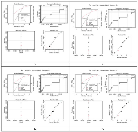
Figure 10.
Prediction error of the MARS models for a sample of some selected elements. Four prediction performances included: the cumulative distribution of prediction errors, residual vs. fitted, residual QQ and GRSq. The values of the performance metrics vary among the elements.
An assessment of results during training and testing phases is presented in Figure 11. The real and predicted values of elemental concentrations revealed variable prediction performances among the selected models, which can be attributed to high variations amongst the modeling techniques used to generate these models. It is worthy to note that all the predicted values shown in this figure are obtained at a 95% confidence interval with respect to their arithmetic mean. Motivated by these findings, the best results of each modeling technique have been considered in the next section.
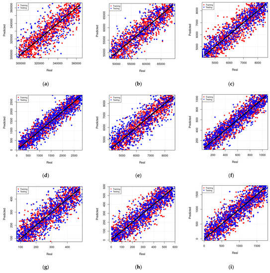
Figure 11.
Assessment under training and testing phases. Real vs. predicted values for selected models are shown, (a) MLR model to predict the concentration of Si as a function of Cu, Zr concentrations, (b) MLR model to predict the concentration of Cu as a function of AL, Fe, Zr, and Ba concentrations, (c) MLR model to predict the concentration of Ni as a function of all other microelements concentrations, (d) RF model to predict the concentration of Al as a function of Cu and Zr concentrations, (e) RF model to predict the concentration of Ti as a function of Ba, Cr, Cu, Y, and Mn concentrations, (f) RF model to predict the concentration of Fe as a function of all other microelement concentrations, (g) MARS model to predict the concentration of Ni as a function of Cu, Zr, and Mn concentrations, (h) MARS model to predict the concentration of Mn as a function of Y, Ni, Fe, Si, and Ba concentrations, (i) MARS model to predict the concentration of Si as a function of all other microelement concentrations.
The results in this study demonstrated that an approach based on EDXRF measurements coupled with machine learning algorithms can predict concentrations of micronutrients in the Taif agricultural soils. An interesting finding was that concentrations of elements that are difficult or impossible to measure directly with the EDXRF device, such as Cu and Cr, can be indirectly predicted with predictor elements present in measurable concentrations. Table 4 shows a comparison of the different models considered in this study using the statistical metrics mentioned above. For the purpose of this comparison the best model generated from each modeling techniques has been used here.
Table 4.
Comparison between different models using statistical metrics.
The assessment provided in this study shows that the MLR, RF, and MARS have different performance predictions. In agreement with Kadkhodazadeh et al. [59], our results indicated that MARS outperforms the other two algorithms (RF and MARS) when the number of explanatory variables is small. Other studies have suggested that the MARS model, as a non-parametric regression approach, has good potential for solving nonlinear problems with high dimensions [60,61]. Subsequently, the MARS algorithm generated basis functions for input variables and then specified regression models by combining basis functions to estimate the output variable [61]. On the other hand, RF revealed higher performance when the number of these variables was large. The random forest has been proved as a machine learning program that is capable of solving regression difficulties in different fields, such as estimating sea surface salinity, nanofluids, groundwater pollution, etc. [62,63]. However, the higher performance of RF requires higher computation times and complexity which in turn encourages researchers to utilize the MLR as a moderate method to make predictions for multivariant variables. The MLR model is commonly used to estimate the linear regression relationship between inputs and target values based on severe data deviations [64,65]. One of the benefits of this model is that it can reduce the changes due to uncertainties. It can be seen from the results that the error values of RF do not follow a general trend which was attributed principally to the reliance of this model on generating several trees and treating data randomly to extract their latent relations.
Finally, the results of the analyses suggested that caution is required when using the presented models. RF models, for example, cannot predict concentrations as low as continuous MLR and MARS models. However, in rare cases, though, MARS and MLR can predict absurd concentrations [14]. An appropriate distribution of concentration in the calibration dataset will facilitate the RF algorithm’s ability to build classes through all ranges. In the present study, RF did not construct sufficient classes for Zr in the upper ranges, which suggests more soil samples are necessary to improve RF’s accuracy. In line with Alder et al. [14], it appears that the continuous models assessed in this study allow for more predictions to be extrapolated. However, a simple linear model, such as MLR, can also be remarkably effective as illustrated in predictions for Zn, and in some cases, Cu. As there is less associated error in predictions, non-linear models such as RF and MARS can be better options overall. Thus, MARS and RF may be roughly suitable to predict concentration ranges, depending on the range of concentrations to be predicted. At lower concentrations, for example, the RF model was more accurate than the MARS model for Cu, but the MARS model performed better at higher concentrations.
Finally, the results reported in this study demonstrated that the proposed machine learning method was able to accurately predict soil microelement concentrations in Taif rose farms, which may save time and effort spent collecting soil samples and analyzing them using traditional methods. Yet, it is noteworthy that the significant concoction amongst these microelements requires a more sophisticated algorithm by which the latent features can be revealed. Motivated by this, future work will focus on applying deep learning algorithms to the collected samples in order to enhance the predictive performance.
4. Conclusions
The primary purpose of this research was to make use of recently improved machine learning techniques to develop general prediction performance for agricultural soils in Saudi Arabia, specifically in the Taif area. EDXRF measurements were used to develop national predictive models that predict the concentrations of 14 micronutrients in soils of Taif rose farms. The models were found to be applicable at farm scale; and capable of predicting concentrations of micronutrients in agricultural soils at farm level, but with varying amounts of error. The study reports that multivariate models can be used to overcome numerous limitations of EDXRF, including high detection limits and an element that cannot be measured directly. Generally, there is no universal ML technique that reliably predicts micronutrient concentrations. The comparative analysis demonstrates that MARS performs well when the number of explanatory variables is small; and RF performs well when the number of variables is large, whereas multivariate linear regression (MLR) should be considered a moderate technique for predicting multivariate variables. This study provides a good foundation for testing the method on a larger dataset of soil samples to create maps of the modeled elements in future studies on soil micronutrient maps in Taif agricultural soils.
Author Contributions
Conceptualization, H.M.A. and M.A.B.; methodology, M.A.B.; software, H.G.Z.; validation, M.A.B., M.A.A. and J.F.A.-A.; formal analysis, M.A.B.; investigation, M.A.A. and E.A.A.; resources, M.M.M.; data curation, M.A.B.; writing—original draft preparation, M.A.B.; writing—review and editing, H.M.A.; visualization, M.A.; supervision, H.M.A.; project administration, H.M.A.; funding acquisition, H.M.A. All authors have read and agreed to the published version of the manuscript.
Funding
This work was financially supported by research project No. (1-441-126) from the Ministry of Education in Saudi Arabia.
Data Availability Statement
All data generated or analyzed during this study are included in this published article.
Acknowledgments
The authors extend their appreciation to the Deputyship for Research and Innovation, Ministry of Education in Saudi Arabia for funding this research work through the project number (1-441-126).
Conflicts of Interest
The authors declare no conflict of interest.
References
- Senapati, S.K.; Rout, G.R. Study of culture conditions for improved micropropagation of hybrid rose. Hortic. Sci. 2008, 35, 27–34. [Google Scholar] [CrossRef]
- Guterman, I.; Shalit, M.; Menda, N.; Piestun, D.; Dafny-Yelin, M.; Shalev, G.; Bar, E.; Davydov, O.; Ovadis, M.; Emanuel, M.; et al. Rose scent: Genomics approach to discovering novel floral fragrance-related genes. Plant Cell 2002, 14, 2325–2338. [Google Scholar] [CrossRef]
- Uggla, M.; Gustavsson, K.E.; Olsson, M.E.; Nybom, H. Changes in colour and sugar content in rose hips (Rosa dumalis L. and Rosa rubiginosa L.) during ripening. J. Hortic. Sci. Biotechnol. 2005, 80, 204–208. [Google Scholar] [CrossRef]
- Kaur, N.; Sharma, R.K.; Sharma, M.; Singh, V.; Ahuja, P.S. Molecular evaluation and micropropagation of field selected elites of R. damascene. Gen. Appl. Plant Physiol. 2007, 33, 171–186. [Google Scholar]
- Nilsson, O. Rosa. In Flora of Turkey and the East Aegean Islands; Davis, P.H., Ed.; Edinburgh University Press: Edinburgh, Scotland, 1997; Volume 4, pp. 106–128. [Google Scholar]
- Naquvi, K.J.; Ansari, S.H.; Ali, M.; Najmi, K. Volatile oil composition of Rosa damascena Mill (Rosaceae). J. Pharmacogn. Phytochem. 2014, 2, 177–181. [Google Scholar]
- Rusanov, K.; Kovacheva, N.; Stefanova, K.; Atanassov, A.; Atanassov, I. Rosa damascena—Genetic resources and capacity building for molecular breeding. Biotechnol. Biotechnol. Equip. 2009, 23, 1436–1439. [Google Scholar] [CrossRef]
- Shohayeb, M.; Arida, H.; Abdel-Hameed, E.S.; Bazaid, S. Effects of Macro-and Microelements in Soil of Rose Farms in Taif on Essential Oil Production by Rosa damascena Mill. J. Chem. 2015, 2015, 935235. [Google Scholar]
- Niu, G.; Rodriguez, S.; Aguiniga, L. Effect of saline water irrigation on growth and physiological responses of three rose rootstocks. HortScience 2002, 43, 1479–1492. [Google Scholar] [CrossRef]
- Bongiovanni, R.; Lowenberg-Deboer, J. Precision Agriculture and Sustainability. Precis. Agric. 2004, 5, 359–387. [Google Scholar] [CrossRef]
- Mertens, J.; Smolder, E. Zinc. In Heavy Metals in Soils: Trace Metals and Metalloids in Soil and Their Bioavailability; Alloway, B., Ed.; Springer: Dordrecht, The Netherlands, 2013; pp. 465–493. [Google Scholar]
- Oorts, K. Copper. In Heavy Metals in Soils: Trace Metals and Metalloids in Soil and Their Bioavailability; Alloway, B., Ed.; Springer: Dordrecht, The Netherlands, 2013; pp. 367–394. [Google Scholar]
- Savvas, D. General introduction. In Hydroponic Production of Vegetables and Ornamentals; Savvas, D., Passam, H.C., Eds.; Embryo Publications: Athens, Greece, 2002. [Google Scholar]
- Adler, K.; Piikki, K.; Söderström, M.; Eriksson, J.; Alshihabi, O. Predictions of Cu, Zn, and Cd Concentrations in Soil Using Portable X-Ray Fluorescence Measurements. Sensors 2020, 20, 474. [Google Scholar] [CrossRef] [PubMed]
- Lemiére, B. A review of pxrf (field portable X-ray fluorescence) applications for applied geochemistry. J. Geochem. Explor. 2018, 188, 350–363. [Google Scholar] [CrossRef]
- Weindorf, D.C.; Zhu, Y.; Chakraborty, S.; Bakr, N.; Huang, B. Use of portable X-ray fluorescence spectrometry for environmental quality assessment of peri-urban agriculture. Environ. Monit. Assess. 2012, 184, 217–227. [Google Scholar] [CrossRef]
- Santana, E.; dos Santos, F.R.; Mastelini, S.M.; Melquiade, F.L. Improved prediction of soil properties with Multi-target Stacked Generalisation on EDXRF spectra. Chemom. Intell. Lab. Syst. 2021, 209, 102431. [Google Scholar] [CrossRef]
- Kilbride, C.; Poole, J.; Hutchings, T.R. A comparison of Cu, Pb, As, Cd, Zn, Fe, Ni and Mn determined by acid extraction/icp-oes and ex situ field portable X-ray fluorescence analyses. Environ. Pollut. 2006, 143, 16–23. [Google Scholar] [CrossRef]
- Kaniu, M.I.; Angeyo, K.H.; Mwala, A.K.; Mwangi, F.K. Energy dispersive X-ray fluorescence and scattering assessment of soil quality via partial least squares and artificial neural networks analytical modeling approaches. Talanta 2012, 98, 236–240. [Google Scholar] [CrossRef] [PubMed]
- Parsons, C.; Grabulosa, E.M.; Pili, E.; Floor, G.H.; Roman-Ross, G.; Charlet, L. Quantification of trace arsenic in soils by fieldportable X-ray fluorescence spectrometry: Considerations for sample preparation and measurement conditions. J. Hazard. Mater. 2013, 262, 1213–1222. [Google Scholar] [CrossRef]
- Caporale, A.G.; Adamo, P.; Capozzi, F.; Langella, G.; Terribile, F.; Vingiani, S. Monitoring metal pollution in soils using portable-XRF and conventional laboratory-based techniques: Evaluation of the performance and limitations according to metal properties and sources. Sci. Total Environ. 2018, 643, 516–526. [Google Scholar] [CrossRef]
- Xia, F.; Fan, T.; Chen, Y.; Ding, D.; Wei, J.; Jiang, D.; Deng, S. Prediction of Heavy Metal Concentrations in Contaminated Sites from Portable X-ray Fluorescence Spectrometer Data Using Machine Learning. Processes 2022, 10, 536. [Google Scholar] [CrossRef]
- Sirsat, M.; Cernadas, E.; Fernández-Delgado, M.; Barro, S. Automatic prediction of village-wise soil fertility for several nutrients in India using a wide range of regression methods. Comput. Electron. Agric. 2018, 154, 120–133. [Google Scholar] [CrossRef]
- Grunwald, S.; Vasques, G.M.; Rivero, R.G. Fusion of soil and remote sensing data to model soil properties. Adv. Agron. 2015, 131, 1–109. [Google Scholar]
- Xu, Y.; Smith, S.E.; Grunwald, S.; Abd-Elrahman, A.; Wani, S.P. Incorporation of satellite remote sensing pan-sharpened imagery into digital soil prediction and mapping models to characterize soil property variability in small agricultural fields. ISPRS J. Photogramm. 2017, 123, 1–19. [Google Scholar] [CrossRef]
- Zhang, Y.; Sui, B.; Shen, H.; Wang, Z. Estimating temporal changes in soil pH in the black soil region of Northeast China using remote sensing. Comput. Electron. Agric. 2018, 154, 204–212. [Google Scholar] [CrossRef]
- Blanco, C.M.G.; Gomez, V.M.B.; Crespo, P.; Ließ, M. Spatial prediction of soil water retention in a Páramo landscape: Methodological insight into machine learning using random forest. Geoderma 2018, 316, 100–114. [Google Scholar] [CrossRef]
- Tziachris, P.; Aschonitis, V.; Chatzistathis, T.; Papadopoulou, M. Assessment of spatial hybrid methods for predicting soil organic matter using DEM derivatives and soil parameters. Catena 2019, 174, 206–216. [Google Scholar] [CrossRef]
- Kovačević, M.; Bajat, B.; Gajić, B. Soil type classification and estimation of soil properties using support vector machines. Geoderma 2010, 154, 340–347. [Google Scholar] [CrossRef]
- Farfani, H.A.; Behnamfar, F.; Fathollahi, A. Dynamic analysis of soil-structure interaction using the neural networks and the support vector machines. Expert Syst. Appl. 2015, 42, 8971–8981. [Google Scholar] [CrossRef]
- Hanna, A.M.; Ural, D.; Saygili, G. Neural network model for liquefaction potential in soil deposits using Turkey and Taiwan earthquake data. Soil Dyn. Earthq. Eng. 2007, 27, 521–540. [Google Scholar] [CrossRef]
- Henderson, B.L.; Bui, E.N.; Moran, C.J.; Simon, D. Australia-wide predictions of soil properties using decision trees. Geoderma 2005, 124, 383–398. [Google Scholar] [CrossRef]
- Dai, F.; Zhou, Q.; Lv, Z.; Wang, X.; Liu, G. Spatial prediction of soil organic matter content integrating artificial neural network and ordinary kriging in Tibetan Plateau. Ecol. Indic. 2014, 45, 184–194. [Google Scholar] [CrossRef]
- Poggio, L.; Gimona, A.; Spezia, L.; Brewer, M.J. Bayesian spatial modelling of soil properties and their uncertainty: The example of soil organic matter in Scotland using R-INLA. Geoderma 2016, 277, 69–82. [Google Scholar] [CrossRef]
- Caubet, M.; Dobarco, M.R.; Arrouays, D.; Minasny, B.; Saby, N.P. Merging country, continental and global predictions of soil texture: Lessons from ensemble modelling in France. Geoderma 2019, 337, 99–110. [Google Scholar] [CrossRef]
- Fathololoumi, S.; Vaezi, A.R.; Alavipanah, S.K.; Ghorbani, A.; Saurette, D.; Biswas, A. Improved digital soil mapping with multitemporal remotely sensed satellite data fusion: A case study in Iran. Sci. Total Environ. 2020, 721, 137703. [Google Scholar] [CrossRef]
- Forkuor, G.; Hounkpatin, O.K.; Welp, G.; Thiel, M. High resolution mapping of soil properties using remote sensing variables in southwestern Burkina Faso: A comparison of machine learning and multiple linear regression models. PLoS ONE 2017, 12, e0170478. [Google Scholar] [CrossRef] [PubMed]
- Emadi, M.; Taghizadeh-Mehrjardi, R.; Cherati, A.; Danesh, M.; Mosavi, A.; Scholten, T. Predicting and Mapping of Soil Organic Carbon Using Machine Learning Algorithms in Northern Iran. Remote Sens. 2020, 12, 2234. [Google Scholar] [CrossRef]
- Wang, B.; Waters, C.; Orgill, S.; Cowie, A.; Clark, A.; Li, L.D.; Simpson, M.; McGowen, I.; Sides, T. Estimating soil organic carbon stocks using different modelling techniques in the semi-arid rangelands of easternAustralia. Ecol. Indic. 2018, 88, 425–438. [Google Scholar] [CrossRef]
- Bian, Z.; Guo, X.; Wang, S.; Zhuang, Q.; Jin, X.; Wang, Q.; Jia, S. Applying statistical methods to map soil organic carbon of agricultural lands in northeastern coastal areas of China. Arch. Agron. Soil Sci. 2020, 66, 532–544. [Google Scholar] [CrossRef]
- Taghizadeh-Mehrjardi, R.; Nabiollahi, K.; Kerry, R. Digital mapping of soil organic carbon at multiple depths using different data mining techniques in Baneh region, Iran. Geoderma 2016, 266, 98–110. [Google Scholar] [CrossRef]
- Fadl, M.A.; Al-Yasi1, H.M.; Alsherif, E.A. Impact of elevation and slope aspect on floristic composition in wadi Elkor, Sarawat Mountain, Saudi Arabia. Sci. Rep. 2021, 11, 16160. [Google Scholar] [CrossRef] [PubMed]
- Farrag, H.F. Floristic composition and vegetation-soil relationships in Wadi Al-Argy of Taif region, Saudi Arabia. Int. Res. J. Plant Sci. 2012, 3, 147–157. Available online: http://www.interesjournals.org/IRJPS (accessed on 6 March 2022).
- Koom, K.; Wiafe-Akenten, J.; Boamah, D. Soil heavy metal pollution along Subin River in Kumasi, Ghana; Using X-ray fluorescence (XRF) analysis. AIP Conf. Proc. 2010, 1221, 101–108. [Google Scholar]
- EPA/ROC. Environmental Information of Taiwan: ROC: Yearbook of Environmental Protection in Taiwan; Environmental Protection Agency (EPA): Taipei, Taiwan, 1998; pp. 82–83.
- Brouwer, N.P. Theory of XRF-Getting Acquainted with the Principles, 2nd ed.; PANalytica: Almelo, The Netherlands, 2006; pp. 8–25. [Google Scholar]
- Hastie, T.; Tibshirani, R.; Friedman, J. The Elements of Statistical Learning, 2nd ed.; Springer: New York, NY, USA, 2009. [Google Scholar]
- Puntanen, S. Handbook of Regression Analysis by Samprit Chatterjee, Jeffrey, S. Simonoff. Int. Stat. Rev. 2013, 81, 330–331. [Google Scholar] [CrossRef]
- Sullivan, W. Decision Tree and Random Forest-Machine Learning and Algorithms: The Future Is Here; CreateSpace Independent Publishing Platform: Scotts Valley, CA, USA, 2018. [Google Scholar]
- Nisbet, R.; Miner, G.; Yale, K. Handbook of Statistical Analysis and Data Mining Applications, 2nd ed.; Academic Press, Inc.: Cambridge, MS, USA, 2017. [Google Scholar]
- Pedregosa, F.; Varoquaux, G.; Gramfort, A.; Michel, V.; Thirion, B.; Grisel, O.; Blondel, M.; Prettenhofer, P.; Weiss, R.; Dubourg, V.; et al. Scikit-learn: Machine Learning in Python. J. Mach. Learn. Res. 2011, 12, 2825–2830. [Google Scholar] [CrossRef]
- Friedman, J.H. Multivariate adaptive regression splines. Ann. Stat. 1991, 19, 1–67. [Google Scholar] [CrossRef]
- Hall, M. Combinatorial Theory, 2nd ed.; Wiley: Hoboken, NJ, USA, 2011. [Google Scholar]
- Shacklette, H.T.; Boerngen, J.G. Element Concentrations in Soils and Other Surficial Material of the Conterminous United States; Government Printing Office: Washington, DC, USA, 1984.
- Al-Mamoori, S.K.; Al-Maliki, L.A.J.; El-Tawel, K.; El-Tawel, K.; Hussain, H.M.; Al-Ansari, N.; Jawad Al Ali, M. Chloride, Calcium Carbonate and Total Soluble Salts Contents Distribution for An-Najaf and Al-Kufa Cities’ Soil by Using GIS. Geotech. Geol. Eng. 2019, 37, 2207–2225. [Google Scholar] [CrossRef]
- Kuhn, M.; Johnson, K. Feature Engineering and Selection: A Practical Approach for Predictive Models, 1st ed.; Chapman and Hall/CRC: Boca Raton, FL, USA, 2019. [Google Scholar] [CrossRef]
- Weller-Fahy, D.J.; Borghetti, B.J.; Sodemann, A.A. A survey of distance and similarity measures used within network intrusion anomaly detection. IEEE Commun. Surv. Tutor. 2015, 17, 70–91. [Google Scholar] [CrossRef]
- Kurz-Kim, J.R.; Loretan, M. A Note on the Coefficient of Determination in Regression Models with Infinite-variance Variables. Dt. Bundesbank, 2007. Available online: https://ideas.repec.org/p/zbw/bubdp1/5574.html (accessed on 6 March 2022).
- Kadkhodazadeh, M.; Valikhan Anaraki, M.; Morshed-Bozorgdel, A.; Farzin, S. A New Methodology for Reference Evapotranspiration Prediction and Uncertainty Analysis under Climate Change Conditions Based on Machine Learning, Multi Criteria Decision Making and Monte Carlo Methods. Sustainability 2022, 14, 2601. [Google Scholar] [CrossRef]
- Bozağaç, D.; Batmaz, I.; Oğuztüzün, H. Dynamic simulation metamodeling using MARS: A case of radar simulation. Math. Comput. Simul. 2016, 124, 69–86. [Google Scholar] [CrossRef]
- Samadi, M.; Jabbari, E.; Azamathulla, H.M.; Mojallal, M. Estimation of scour depth below free overfall spillways using multivariate adaptive regression splines and artificial neural networks. Eng. Appl. Comput. Fluid Mech. 2015, 9, 291–300. [Google Scholar] [CrossRef]
- Wang, Z.; Wang, Y.; Zeng, R.; Srinivasan, R.S.; Ahrentzen, S. Random Forest-based hourly building energy prediction. Energy Build. 2018, 171, 11–25. [Google Scholar] [CrossRef]
- Gholizadeh, M.; Jamei, M.; Ahmadianfar, I.; Pourrajab, R. Prediction of nanofluids viscosity using random forest (RF) approach. Chemom. Intell. Lab. Syst. 2020, 201, 104010. [Google Scholar] [CrossRef]
- Juneng, L.; Latif, M.T.; Tangang, F. Factors influencing the variations of PM10 aerosol dust in Klang Valley, Malaysia during the summer. Atmos. Environ. 2011, 45, 4370–4378. [Google Scholar] [CrossRef]
- Huangfu, W.; Wu, W.; Zhou, X.; Lin, Z.; Zhang, G.; Chen, R.; Song, Y.; Lang, T.; Qin, Y.; Ou, P.; et al. Landslide Geo-Hazard Risk Mapping Using Logistic Regression Modeling in Guixi, Jiangxi, China. Sustainability 2021, 13, 4830. [Google Scholar] [CrossRef]


Publisher’s Note: MDPI stays neutral with regard to jurisdictional claims in published maps and institutional affiliations. |
© 2022 by the authors. Licensee MDPI, Basel, Switzerland. This article is an open access article distributed under the terms and conditions of the Creative Commons Attribution (CC BY) license (https://creativecommons.org/licenses/by/4.0/).