Abstract
Considering that the relationships between agrometeorological drought indices and the impact of agricultural drought in Slovenia are not yet well understood, the aim of this study was to make an indicative evaluation of the success of selected drought indices, addressing topsoil layer and vegetation condition, in detecting drought in agriculture. In this study, the performance of two established drought indices—the SPEI (standardised precipitation evapotranspiration index) and the VHI (vegetation health index)—was evaluated with respect to yield values calculated with the LINGRA-N model, specifically, the ratio between actual and potential transpiration, also known as drought factor (TRANRF), actual root zone water content (SMACT), leaf area index (LAI), reserve dry weight (WRE), and root dry weight (WRT). The two grassland species selected for analysis were Dactylis glomerata L. (dg) and Lolium perenne L. (lp). For the period 2002–2020 or 2015–2020, three farm sites in Slovenia were considered for evaluation, with two farms at a higher altitude site and one farm at a lower altitude site in the Alpine region. Evaluation of the yield data with the drought indices showed that the r2 values of the linear regression for the selected years with the highest drought impacts (2003, 2013, and 2017) were highest between the two SPEI indices (SPEI-2, SPEI-3) and the model variables TRANRF, SMACT, and WRT, with r2 higher than 0.5 and statistically significant for the lower situated farm in 2013. For 2003 and 2017, the r2 values were less significant as well as for the model variable WRE for all three years selected for analysis (2003, 2013, and 2017).
1. Introduction
Drought is a complex naturally occurring phenomenon, causing significant hydrological imbalances that adversely affect land resource production systems. It can be examined from different perspectives (meteorological, agricultural, hydrological, and socio-economic drought), depending on the impacts it induces. Agricultural drought affects plants and crops, for example, by reducing vegetation productivity, which can result in extensive crop failure. This type of drought is becoming a constant hazard to agricultural production in Europe and Slovenia alike. In the EU and UK, economic losses due to drought in recent decades (1981–2010) have been estimated at approximately 9.0 billion euros per year, with the largest share of losses (39–60%) related to agriculture [1]. In most of Europe, climate change, especially rising air temperatures and the associated increased evaporation and changes in steady precipitation patterns, have exacerbated drought problems in recent decades [2]. Particularly, the summer droughts of 2003, 2015, and 2018 have raised concerns about the vulnerability of the European water resources and water balance to climate change [1].
The data show that annual rainfall is declining in many regions of central and southern Europe [1]. In Slovenia and surrounding areas, the last three decades have been characterised by changes in agricultural drought [3]. Almost every year, different periods of drought occur during the growing season, causing agricultural plants to be under drought stress. Since 1990, agricultural droughts have become more frequent and intense. In addition, recent droughts have been occurring in areas where water shortage was not an issue in the past. An example of this is the Alpine mountain region, which is experiencing severe drought related impacts despite a humid climate [4,5,6]. Drought impacts in the Alpine region mostly occur in summer and early autumn regardless of region, climatic condition, or altitude [5]. Agriculture and livestock farming impacts are even more frequently reported compared to the whole of Europe, especially in the southern region. More than half of all reports are related to reduced productivity of annual or permanent crop cultivation and agricultural yield losses. In Slovenia, these categories are related to 96% of all reported impacts in agriculture and livestock farming on the country level [5]. As elsewhere, these impacts due to drought are caused by prolonged periods with unfavourable distribution and lack of precipitation in combination with high temperatures, especially in summer when enhanced evapotranspiration during heat waves can rapidly reduce surface water supply [6]. In addition to so-called flash droughts in summer, changing the characteristics of an otherwise gradually developing phenomenon, droughts now also occur in typically wetter seasons—autumn and winter. The intensity and frequency of drought is expected to increase with climate change, especially in the south-western part of Europe, whereas an opposite signal is projected for north-eastern Europe [1]. This also includes the higher probability for future droughts in the Alpine region, mainly in the summer months [7,8].
In terms of landscapes and plant species, the Alps are among the richest and diverse regions of Europe and are thus one of the highest conservation priorities in Europe. Climate change and increasing incidence of extreme events are an additional threat to Alpine biodiversity. Some changes can already be observed such as the migration of the Alpine plant species upward and replacement by more competitive species from lower altitudes [9]. In the context of plant productivity, there is strong evidence that increased frequency and magnitude of extreme climate events such as drought considerably affect plant performance [10]. Plants can efficiently cope with sporadic stress, but prolonged stress usually leads to irreversible damage [11]. Drought can limit plant photosynthetic capacity and growth by decreasing soil moisture. The severity of these effects tends to increase with altitude in humid temperate mountains such as the European Alps, where precipitation and air humidity are typically constantly high compared with lower altitudes [10]. In addition to this, mountains are a nutrient-limited ecosystem, meaning that drought can limit plant growth by reducing the microbial activity in the soil. Upland plant species thus depend strongly on relatively high precipitation and high soil moisture, so their growth and reproduction are more susceptible to short periods of drought. Alpine and pre-Alpine landscapes are dominated by grasslands, ranging from intensive grasslands in the lower-elevation areas to highly diverse mountain pastures for beef and dairy production typical in higher-elevation areas [12]. Alpine grasslands provide a number of services that go beyond national borders including fodder production, water retention and purification, storage of nitrogen and carbon as well as space for recreation [13]. Due to a very heterogeneous plant composition, certain mountain grasslands represent some of the species-richest ecosystems in Europe [14,15]. Maintaining traditional agricultural practices such as pasture grazing is thought to be beneficial for conserving Alpine biodiversity [9]. On the other hand, measures such as irrigation and the introduction of seed mixtures including drought tolerant species may be particularly important in the southern part of the Alps (including Slovenia), where drought is likely to decrease the biomass production from grassland in the future [12].
The damaging character of agricultural droughts in the past and increasing probability in future projections in the Alpine region confirm the need for area-wide monitoring, in order to improve drought preparedness and contribute to risk prevention and management practices (e.g., implementing technical measures in a timely manner). The Alpine Drought Observatory Project addresses this need with the aim to develop a platform for improved and harmonised drought monitoring for a broader Alpine area, with indices tailored to Alpine area specifics [16]. There are already some examples of good practices of regional drought monitoring tools (e.g., European Drought Observatory), which include different indices based on meteorological observations, modelled data, or remote sensing data. In combination with information on exposure and vulnerability, drought indices are essential for tracking and warning of the possible drought related effects, impacts, and outcomes [17]. To use a specific drought index in this manner, it is necessary to assess the performance of the index to detect and monitor different types of drought. In the context of agriculture and plant productivity, particularly relevant for the Alpine region, this implies the ability of a targeted index to show where vegetation growth is water-limited and can be achieved through evaluation against various environmental datasets. Good examples of this are two recent studies performed in Bavaria, the first one assessing the performance of the standardised precipitation index (SPI) and the standardised precipitation evapotranspiration index (SPEI) using carbon flux data (gross primary production (GPP) and net ecosystem exchange (NEE)) [18], and the second one evaluating drought indices, namely the temperature condition index (TCI), the vegetation condition index (VCI), and the vegetation health index (VHI) with soil moisture and agricultural yield anomalies [19]. In both studies, a linear correlation analysis between drought-index datasets and chosen environmental variables was performed. In the first study, evaluation with carbon flux data showed that the average r2 values of a pixel-wise linear regression for the growing season for the period 1980–2010 between SPEI, SPI, and VCI with NEE were 0.26, 0.07, and 0.37, respectively, while the average r2 values for SPEI, SPI, and VCI with GPP were lower (0.03, 0.04, and 0.14, respectively) [18]. The second study found that the TCI and VHI correlated strongly with soil moisture and agricultural yield anomalies. Over the growing season in the period 2001–2020, the values of the Bravais–Pearson correlation coefficient of SMI with TCI were 0.54, with VHI 0.48, while the one between SMI and VCI was lower at 0.27. Positive correlations of varying strength were found between drought indices and yield data for different crops, ranging between 0.45 (VCI) and 0.49 (VHI) [19]. These results suggest that remote sensing-based vegetation indices in particular have the potential to detect agricultural drought. Since agricultural drought is usually affected by a variety of complex external and internal self-regulating mechanisms such as climate, biophysical conditions, and human activities [20], a variety of evaluation approaches exist in this respect [21]. Examples of these are using local qualitative observations of crop phenological development, in situ soil/plant measurements, crop yield, damage reports of drought impacts on vegetation, and different types of remote sensing data for comparison, but in Slovenia, these are either not collected regularly and systematically or are limited by a short temporal period of observation and on limited experimental plots. Some of these gaps can be filled with a more experimental approach using vegetation (grassland) modelling, which is the purpose of this case study. Finally, combining field measurements and laboratory data to assist in evaluating the ability of drought indices to detect agricultural drought would further improve the application prospects of their use.
2. Materials and Methods
2.1. Area Description
In the case study of the Slovenian Alpine region, we considered three farms. Information on grassland management was provided by the owners of the farms. The first one (Planica-Farm1e) is situated at a higher altitude at about 650 m above sea level. The permanent meadows are mowed three times per year; in 2020, the mowing dates were 21 May, 23 July, and 20 September. Manure (about 20–30 m3/ha) is applied once per season (in April 2020), the farm is organic, and does not use other fertilizers. The neighbouring farm is intensive (Planica-Farm1i). On Farm1i, they mow four times per year; the mowing and fertilising regime is represented in Table 1 and is due to its intensity, atypical in this part of the Alpine area.

Table 1.
Review of days of fertilisation, amounts of fertilisers, and fertilisation methods based on 2020 data.
According to the objective climate classification of Slovenia [22], the climate type at Farm1e and Farm1i is the moderate climate of the hilly region (Figure 1), which covers lower pre-Alpine hills. Monthly mean temperature of winter months is below 0 °C while monthly mean temperature in July (the warmest month) is above 18 °C, which means that the seasonal amplitude is rather high. The amount of precipitation over the year is neither high nor low. Two not very significant precipitation peaks can be observed from the annual precipitation cycle, the first one in June (149 mm), and the second one in the autumn months (151 mm). In winter (January and February), the monthly precipitation is the lowest (76–77 mm). Most of the snow falls in winter, while some also falls in autumn and spring. The amount of precipitation and the amplitude of the annual temperature cycle both indicate continental climate characteristics.
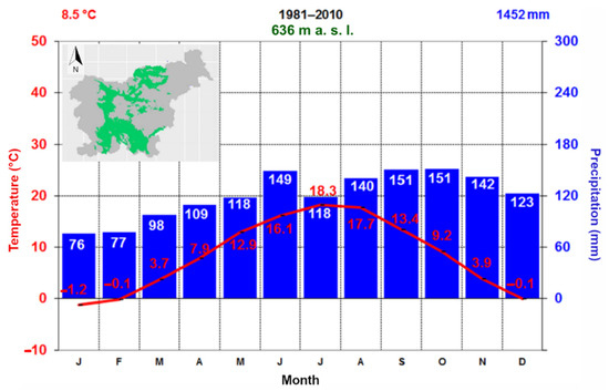
Figure 1.
Climograph of the moderate climate of hilly region, climate type at Farm1e and Farm1i (Reprinted with permission from Ref. [22]. Copyright 2016, Katja Kozjek). Numbers in upper corners represent average annual temperature (left) and precipitation (right).
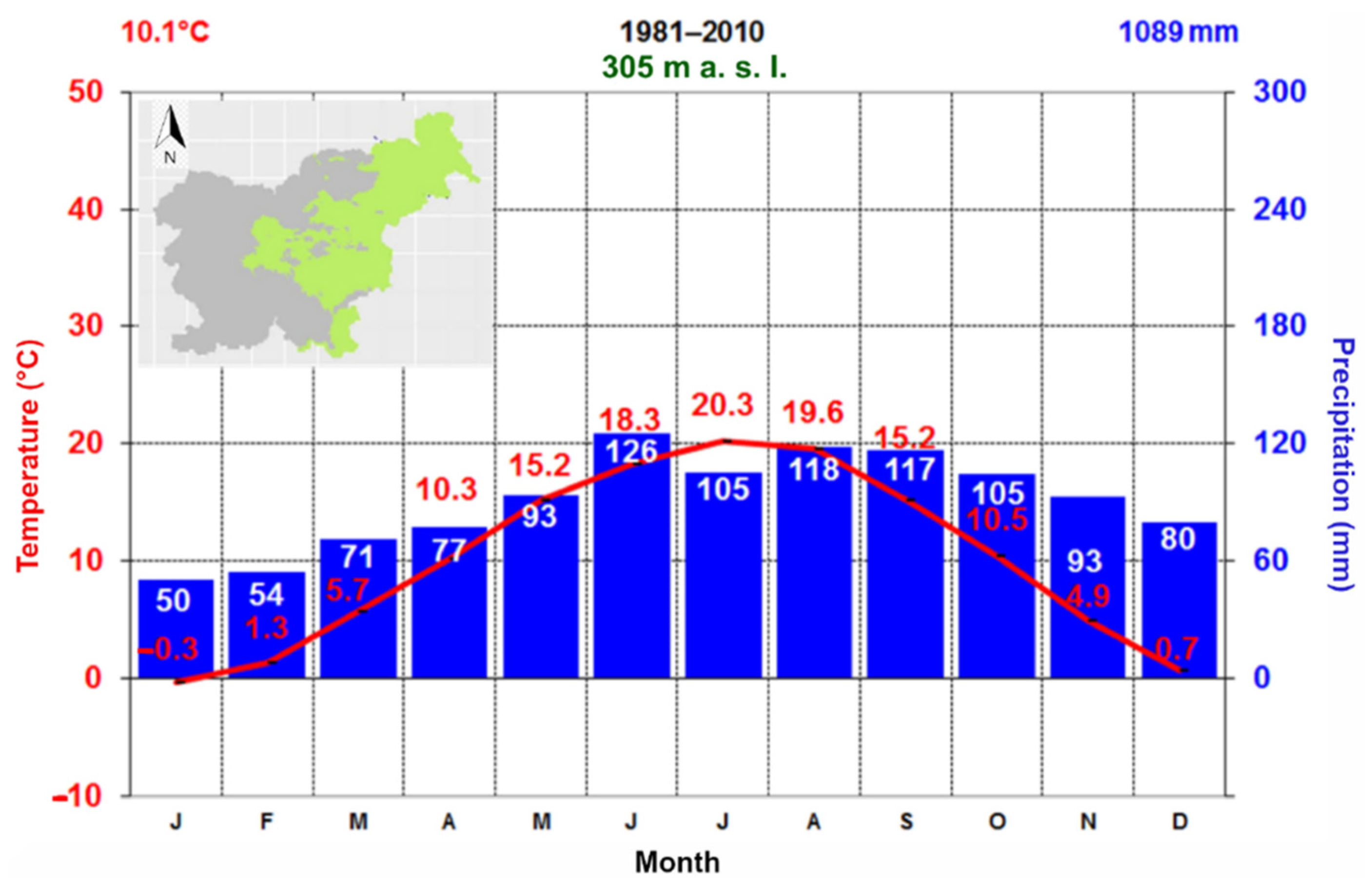
The third farm (Svecina-Farm2) is located in the lowlands at about 355 m above sea level. Their fertilization and mowing regime are also represented in Table 1. The climate type at Farm2 is the subcontinental climate (Figure 2), covering the most continental and driest region in Slovenia [22]. Annual precipitation mean in this region is slightly above 1000 mm, while monthly precipitation amounts range from 50 mm in January to 126 mm in June. In summer, the maximum temperature can be very high, thus the monthly mean temperature in July is above 20 °C. On the other hand, the minimum temperature in winter can drop fairly low, consequently, the monthly mean temperature in winter months is around 0 °C. As a result, the seasonal amplitude is greater than 20 °C. Snow mostly falls in winter. Both temperature and precipitation regime in this region show continental climate characteristics but they are not as strongly pronounced as in a typical continental climate. Though there are some similarities between the two climate types in our case study area, the subcontinental climate is drier and warmer compared the moderate climate of the hilly region and the continental influence is more pronounced.
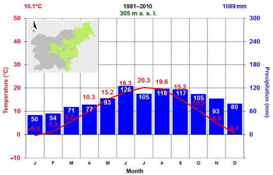
Figure 2.
Climograph of the subcontinental climate, climate type at Farm2 (Reprinted with permission from Ref. [22]. Copyright 2016, Katja Kozjek). Numbers in upper corners represent average annual temperature (left) and precipitation (right).
2.2. Modelling of the Grassland Growth Parameters and Yield
The LINGRA-N model ([23,24,25,26]—see the last one for all equations and to understand the model flow)—was used for modelling. In the model, the growth rate is determined according to solar radiation or air temperature, depending on which one prevails based on the integrated thresholds. The growth simulation in the model begins when the 10-day moving average of the daily air temperature exceeds the threshold temperature. The natural development cycle of grassland does not have the usual characteristics of crops, as regular mowing interrupts it. Therefore, the LINGRA-N model does not simulate the developmental stage of the plant as a phenological phase, but nevertheless uses the developmental stage (DVS) to mimic the simulation of plant development for comparisons between locations. This is defined as the temperature sum of average daily air temperatures above 0 °C from the beginning of the year, divided by the parameter TSUM1 (°C), which on average represents the temperature sum required for flowering to occur. There are four sets of input data relating to weather conditions, soil condition, ecophysiology, and grassland management. Atmospheric concentration of CO2 was set at 410 ppm, irrigation was not simulated, and water balance and growth were re-simulated each year.
In the past, the model was calibrated for two sites in Slovenia (Jablje and Rakičan) using field trial data. The simulations for Dactylis glomerata L. (dg) and Lolium perenne L. (lp) matched the data best, the index of agreement between predicted and observed values was 0.8, showing very good agreement (see [27] for more details). Since longer datasets for grassland crops are not available for the selected farms in the case study area, the model cannot be recalibrated, and mainly, previously calibrated plant parameters were used.
A review of phenological data from the Slovenian Environment Agency [28] revealed that there are three phenological stations near the selected farms (Table 2—sign F): Hočko Pohorje (F) is located at a higher altitude and is therefore well representative of Farm1e and Farm1i, while Starše and Kadrenci are comparable and more representative of Farm2. Flowering dates were compared with the sum of all positive average daily air temperatures from 1 January to the day of flowering. Flowering in the lowlands of the case study occurs sometime between 27 April and 1 May, which equals to a temperature sum of about 610 to 650 °C. At the higher Hočko Pohorje, the flowering phase occurs with a delay of several days, around 15 May, depending on the conditions in a single year. The corresponding temperature sum averages 873 °C, which is much higher than the sum for Farm2. The model accounts for the temperature sum, so 630 °C was used for Farm2 and 850 °C for the higher elevation Farm1e and Farm1i due to model better response to slightly lower values (showed in previous studies).
Table 2.
Meteorological and phenological stations in the vicinity of the selected farms.
As meteorological input, the data on daily maximum and minimum air temperatures, precipitation, wind speed, solar radiation energy, and morning value of partial vapor pressure are required. Datasets are available from the archive [28] for two meteorological stations near the selected farms (Table 2—sign M). Maribor Airport can be used for Farm2 with all data available for the period 2002–2020. For the higher elevation Farm1e and Farm1i, conditions are better reflected in Hočko Pohorje (M), where data for the period 2015–2020 are available with the exception of vapour pressure and solar radiation. Partial vapour pressure values can be calculated from morning values of air temperature and relative humidity according to partial and saturated vapour pressure equations of [29]. For solar radiation, the data from Maribor Airport, located below Hočko Pohorje, are more representative than calculations from the daily maximum and minimum temperatures, where quite large errors can occur.
In the soil data file, we set the field capacity for Farm1e and Farm1i to 0.3 and the wilting point to 0.15, and for Farm2 to 0.35 and 0.18, respectively. All values were estimated for the topsoil from the nearest measurements in similar soils by the Infrastructure Centre for Pedology and Environmental Protection (ICPVO). Soil temperature at the beginning of growth was set at 5°C. For mowing and fertilising, we used data for 2020 as a rough approximation, which was better than letting the model determine these dates itself.
In addition to yield model values throughout the period (daily and annual values), we analysed some other model outputs such as the ratio between actual and potential transpiration, also known as drought factor (TRANRF), actual root zone water content (SMACT—determined as the ration between the sum of the rate of net influx through the upper root zone boundary, the rate of net influx through the lower root zone boundary and the actual transpiration rate of crop, and the actual rooting depth), leaf area index (LAI—the one-sided green leaf area per unit ground surface area), reserve dry weight (WRE—the mass of the storage of carbohydrates), and root dry weight (WRT).
2.3. Drought Indices Based on Reanalysis and Remote Sensing
Two multi-scalar indices were selected for evaluation with the modelled grass yield based on their characteristics (addressing topsoil layer and vegetation condition) and reported ability to identify and monitor agricultural drought; the standardised precipitation evapotranspiration index (SPEI) and the vegetation health index (VHI).
SPEI [30] uses the basis of SPI [31] but includes an evapotranspiration component, allowing the index to account for the effect of evapotranspiration development through a basic surface water balance calculation (precipitation subtracted by potential evapotranspiration). It represents a standardised measure of what a certain value of surface water balance over the selected time period means in relation to the expected value of surface water balance for the same period. It can be used on different timescales. The values of the SPEI around 1 represent approximately one standard deviation of the surplus in surface water balance (wet conditions), while the value of −1 is approximately one standard deviation of the deficit (dry conditions). Drought is usually defined as a period when SPEI values fall below −1.
The SPEI was calculated with a daily temporal resolution using normalised generalised logistic distribution with limits set between −3 and 3 [32] using 1981–2020 as the reference period for distribution fitting. The name of the indicator is usually modified to include the time scale (accumulation period), which corresponds to the length of the rolling time window over which the total surface water balance is calculated: two months or 60 days for SPEI-2 and three months or 90 days for SPEI-3. This approach varies slightly from the more common approach, where SPEI is calculated monthly according to the calendar month. Due to standardisation, SPEI is applicable for all climate regimes and can be used to identify and monitor conditions associated with a variety of drought impacts including agriculture when shorter timescales (2–3 months) are considered. SPEI-2 and SPEI-3 were thus selected for the evaluation.
The equation below shows the general calculation of the SPEI:
where SPEIikdy is the z-value for the grid cell i over time scale k for day d and year y; SWBikdy is the surface water balance value for grid cell i over time scale k for day d and year y; SWBikd is the mean for grid cell i over time scale k for day d over the 30-year reference period; and σikd is the standard deviation of grid cell i over time scale k for day d over the 30-year reference period of 1981–2010. As surface water balance data are usually not normally distributed, especially on time scales of 12 months or less, a transformation using generalised logistic distribution is applied.
Precipitation and potential evapotranspiration data used as input data for the calculation of the SPEI were downscaled from ERA5 reanalysis to 5 km resolution [33] using quantile mapping based on a UERRA reanalysis dataset [34]. Precipitation data were downscaled directly, whereas potential evapotranspiration was derived from other downscaled variables (temperature, wind speed, humidity, solar radiation) using the Penman–Monteith method.
VHI [35,36] is one of the first indices used to monitor and identify drought-related agricultural impacts using remotely sensed data. Data in the visible, infrared, and near-infrared channels are used to identify and classify stress to vegetation due to drought. VHI is based on a combination of products extracted from vegetation signals, namely, the normalised difference vegetation index (NDVI) and from the land surface temperature (LST), both derived from MODIS satellite data. The NDVI is based on daily MOD09GQ [37] and LST on daily MOD11A1 [38] products. The spatial resolution of the VHI is 231 m, therefore the original 1000 m resolution of the MOD11A1 LST is downscaled to 231 m of the MOD09GQ reflectance.
The VHI consists of two components (i.e., VCI and TCI). The VCI is defined as follows [35,36]:
where NDVI is the smoothed 4-day NDVI, NDVImin, and NDVImax the corresponding multiyear minimum and maximum. The TCI is defined as follows [35,36]:
where T is the smoothed 4-day temperature, defined by the LST, and Tmin and Tmax are the corresponding multiyear minimum and maximum. The combination of VCI and TCI results in the VHI [35,36]:
where α defines the share of VCI and TCI in the VHI, which was set at 0.5 assuming equal weight of both indices. The values of VHI are provided as aggregated four-day measures, ranging from 0 (severe vegetation stress) to 100 (very favourable conditions). VHI thus relies on a negative correlation between NDVI and LST, since increasing land temperatures are assumed to act negatively on vegetation and cause stress.
Grid cells corresponding to the locations of the farms were used for evaluation with modelled grassland. In the case of the SPEI grid, the entire farmland is located inside one cell, whereas in the case of the VHI grid, the farmland extends over several cells. For VHI evaluation, we selected the cells that best represent permanent grassland (grid cells with the largest share of permanent grassland) based on the information provided by farm owners and drone scan images (Figure 3 and Figure 4).
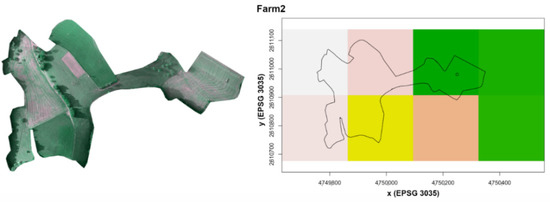
Figure 3.
Drone scan image of Farm1e (left) and selected grid cell (marked with a small circle) for remote sensing based VHI in the permanent grassland area on Farm1e (right—colours are not important, only cell layout is represented).
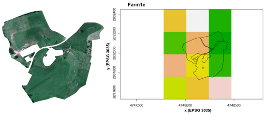
Figure 4.
Drone scan of Farm2 (left) and selected grid cell (marked with a small circle) for remote sensing based VHI in the permanent grassland area on Farm2 (right—colours are not important, only cell layout is represented).
2.4. Statistical Analysis
First, the annual values of modelled yield were compared with data from the Statistical Office of the Republic of Slovenia (SURS) on grassland yields, which are averaged values for all types of permanent grassland throughout Slovenia and with data gained from the assessments of agricultural advisors from the Institute of Agriculture and Forestry Maribor (KGZ MB), collected on the basis of field visits in the observed Alpine region. SURS data on the national scale were only shown to see whether regional and local data formed similar inter-annual variation. Index of agreement was used to compare annual modelled and assessed values.
Second, as from the above three sets, only model results are available on daily scale, modelled data (TRANRF, SMACT, WRE and WRT) for Farm2 with calibration for dg and lp in Jablje were compared with SPEI-2, SPEI-3, and VHI data using basic statistical methods. The main goodness-of-fit measure we calculated was the coefficient of determination (r2), which represents the proportion of total variance that can be explained by the regression model. The coefficient of determination values can range from 0 to 1, where higher values of r2 indicate better agreement between the compared data. Statistical significance (p) was determined using the t-test.
3. Results
3.1. Field Data and Model Simulations
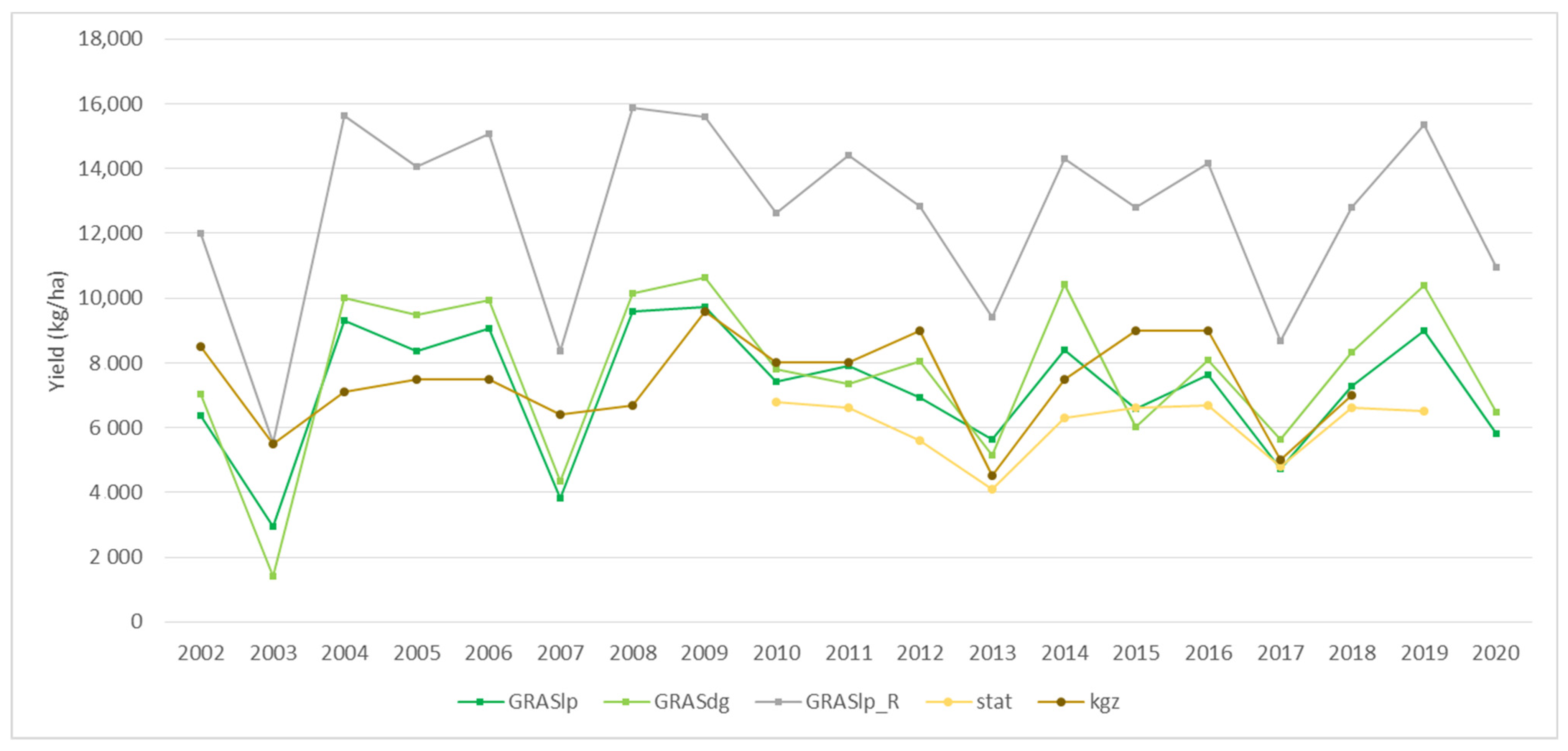
Model results of grassland yield for Farm2 were on an annual scale compared to estimated yields in the lower part of the Slovenian Alpine region and to national yield data from the statistical office (Figure 5). The latter (stat) was only used to compare the approximate level of yields, showing slightly lower values and lower variability within the data for the national level due to averaging. Furthermore, even the variability of yields of individual species is expected to be higher than the variability of yields of the whole meadow, even more so when we talk about all meadows in this area. Comparing the modelled yields to assess for the area (kgz), it can be seen that the calibration for Rakičan (GRASlp_R) is not suitable for use at this location, and yields were very overestimated. For the other two versions with parameters calibrated for Jablje, the modelled results agreed quite well with the assessed yields, with an index of agreement of 0.4 for the better one (GRASlp) and r2 of around 30% for both of them. This is how we decided to only use the mentioned two calibrations for further comparisons.
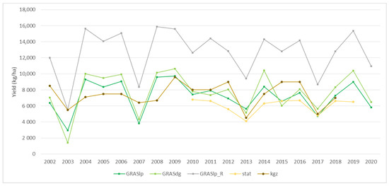
Figure 5.
Model results of annual grassland yield for Farm2 using the parameter set calibrated for Dactylis glomerata and Lolium perenne in Jablje (GRASdg and GRASlp), Lolium perenne in Rakičan (GRASlp_R); annual grassland yield from SURS (stat), and annual yield based on the KGZ MB agricultural advisors’ observations (kgz).
The model showed much lower yields than kgz in the years 2003, 2007, and 2015. On the other hand, the yield was much higher than kgz in 2008. The agreement between modelled and kgz yields was mainly very good from 2009 onward. For the two farms (Farm1e and 1i) at higher elevation, it was also observed that the two calibrations for Jablje were much better, although we had a very short period of meteorological data, only six years, which led to a less reliable comparison (not shown).
The model was after the described comparison further used with Jablje calibration to calculate the annual values of radiation use efficiency (RUE), which is defined as the ratio of total aboveground dry matter to total intercepted solar radiation. It responds intensely to drought when the efficiency of radiation use is much lower. Therefore, the annual variability of RUE is very similar to the variability of the drought factor (TRANRF) (not shown). Low values of RUE and TRANRF were obtained in the years 2003, 2007, 2013, 2015, 2017, and 2020. Roughly speaking, when annual conditions are drier than usual, RUE values are lower than 1.1 gDM/MJ PAR and TRANRF values are lower than 0.9. Based on this information (and yield values), we decided in which year we would observe the development using daily modelled data. Years 2017, 2018, and 2019 were chosen, showing various conditions from the dry with low yield in 2017 to the high yield in 2019.
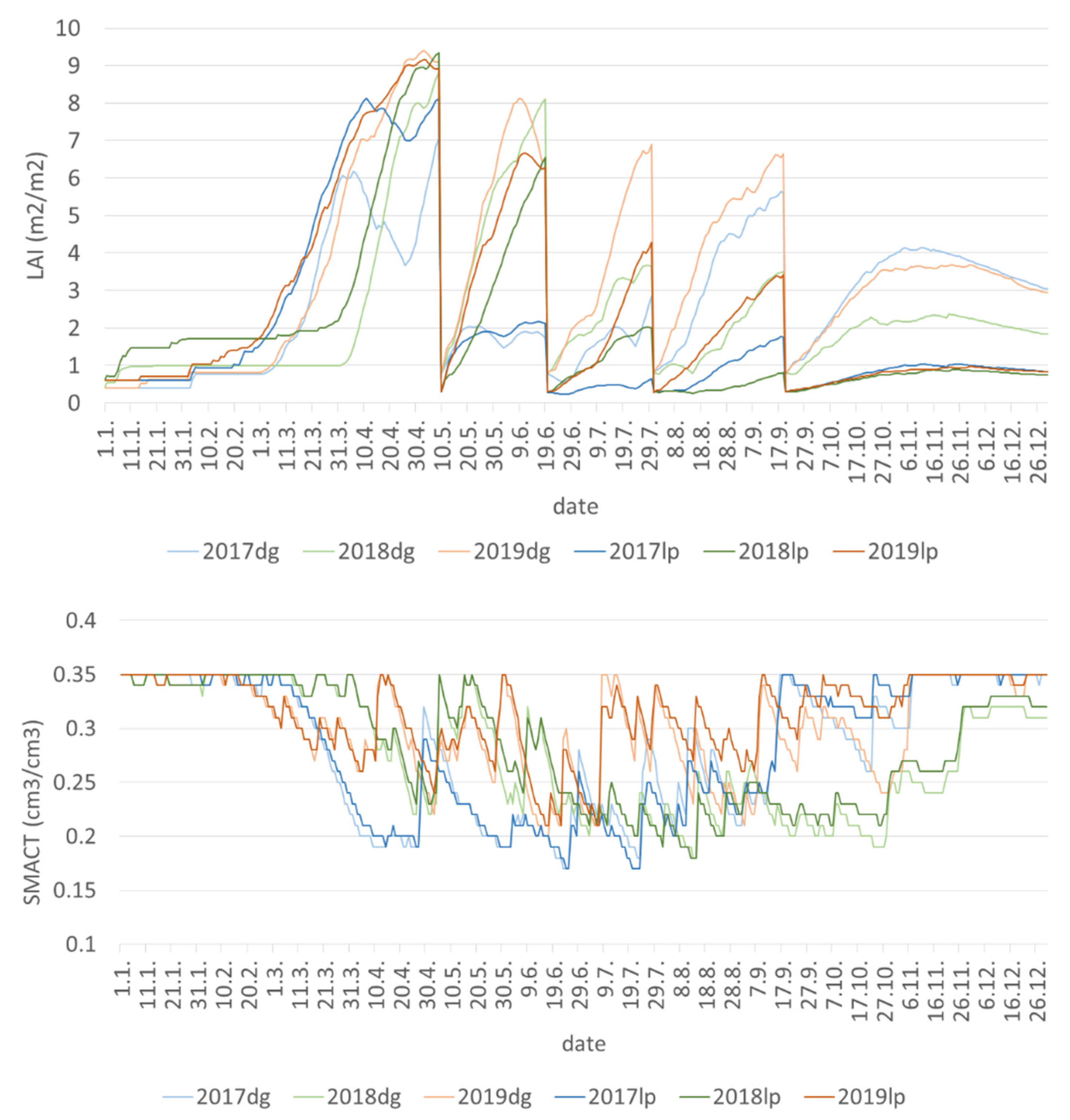
Leaf area index (LAI) showed poor development between the first and second mowing on Farm1e in 2017 and between the second and third mowing on Farm1i (not shown). Low soil water content (SMACT) and very low TRANRF values were also observed during this period, most evident between 1 and 20 April. In 2018, water scarcity was not as pronounced and started mainly after 10 July. On Farm2 (Figure 6), the poor performance of LAI in 2017 was also very noticeable (especially for dg) from 1 April. Water scarcity continued practically throughout the 2017 growing season. After the first mowing, both grasses (dg and lp) recovered only slightly in the model, after the second mowing, lp was in dormancy and dg was already developing somewhat, after the third mowing, dg recovered completely and lp barely, and after the fourth mowing, lp still did not recover. During the dry period, the roots did not reach their full potential, although assimilates were distributed there due to the lack of water. In 2017, this was most clearly reflected in the root dry weight (WRT—not shown) of lp. In general, lp is no longer active after the fourth mowing and after each mowing, the difference between lp and dg continues to increase. The effect of drought was also evident in both species in 2018 after the second mowing. The most optimal year was 2019 when it was only slightly dry after the second mowing.
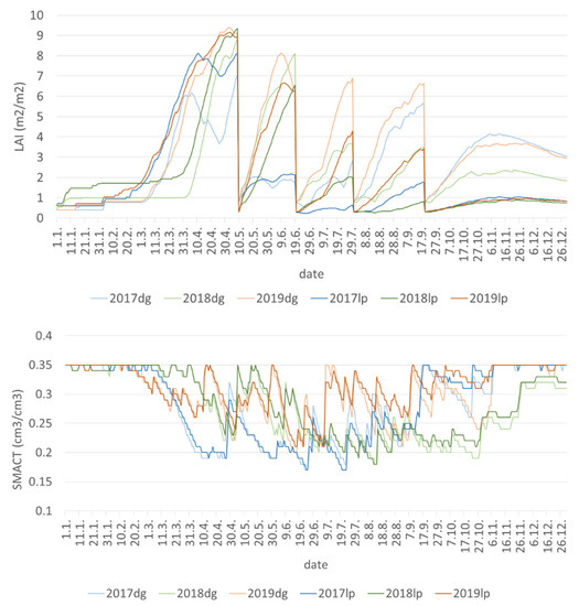
Figure 6.
Daily values of LINGRA-N model results for the period 2017–2019 for Farm2 using parameter set calibrated for Dactylis glomerata in Jablje (dg) and Lolium perenne in Jablje (lp). (Above): leaf area index (LAI), (below): actual soil moisture (SMACT).
3.2. Evaluation of Drought Indices Using Model Results
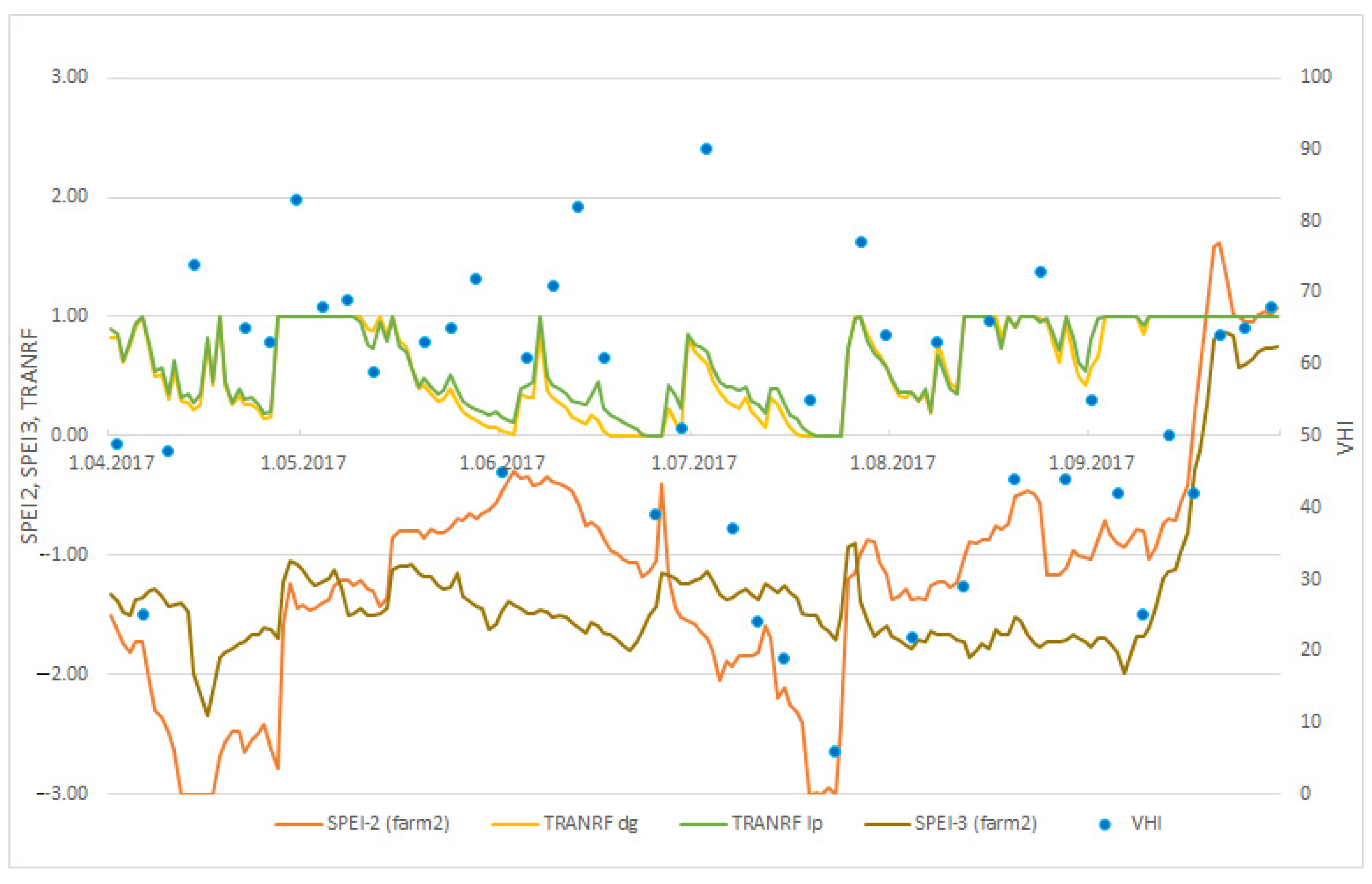
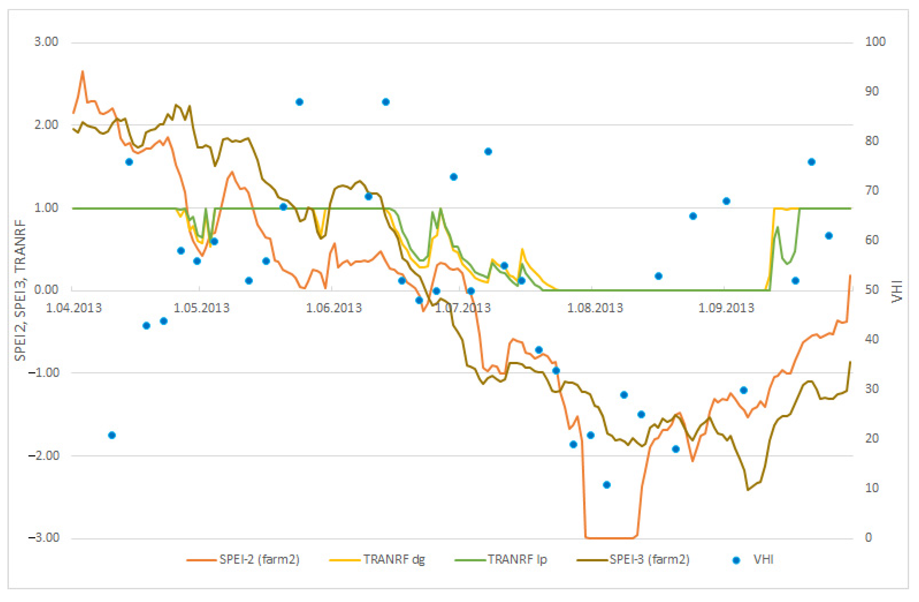
Time series comparison of the model results for Farm2 and SPEI-2, SPEI-3, and VHI indices were performed for dry years 2017, 2013, and 2003 to observe the correlation of indices under the most significantly dry conditions. In the previous section, the model results of three consecutive years were analysed, with the first year having the lowest yield and last year having the highest yield, taking into account one drought-impacted year (year 2017). However, in this section, the emphasis is solely on the years of data with high drought impact, considering that there are also numerous other factors that make the comparison of indices difficult and that the purpose was to validate drought. During the April–September 2017 period (Figure 7), the agreement between the indices was strongest during the summer months of June, July, and August, with a decreasing trend between 10 June and 1 July. There was a sudden increase in early July, followed by a steady decline toward the end of the month. Although the time series of the VHI index had some intervals of missing data, its trend was consistent with other indices, with a local maximum around 10 June, a global maximum around 1 July, and a decreasing trend first toward the end of June and then toward the end of July. Comparison of the results for 2013 (Figure 8) showed the best agreement between the indices in the summer period from late June to mid-September. Both the SPEI-2 and SPEI-3 indices caught two local minima in the TRANRF in early May and late June. The VHI index also showed a similar pattern.
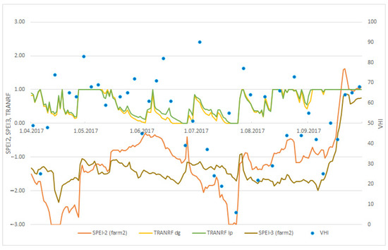
Figure 7.
Time series of the LINGRA-N model results of drought factor (TRANRF) using the parameter set calibrated for Dactylis glomerata in Jablje (dg) and Lolium perenne in Jablje (lp); time series of drought indices (VHI, SPEI-2 and SPEI-3) for Farm 2, all for 2017.

Figure 8.
Time series of the LINGRA-N model results of drought factor (TRANRF) using the parameter set calibrated for Dactylis glomerata in Jablje (dg) and Lolium perenne in Jablje (lp); time series of drought indices (VHI, SPEI-2, and SPEI-3) for Farm2, all for 2013.
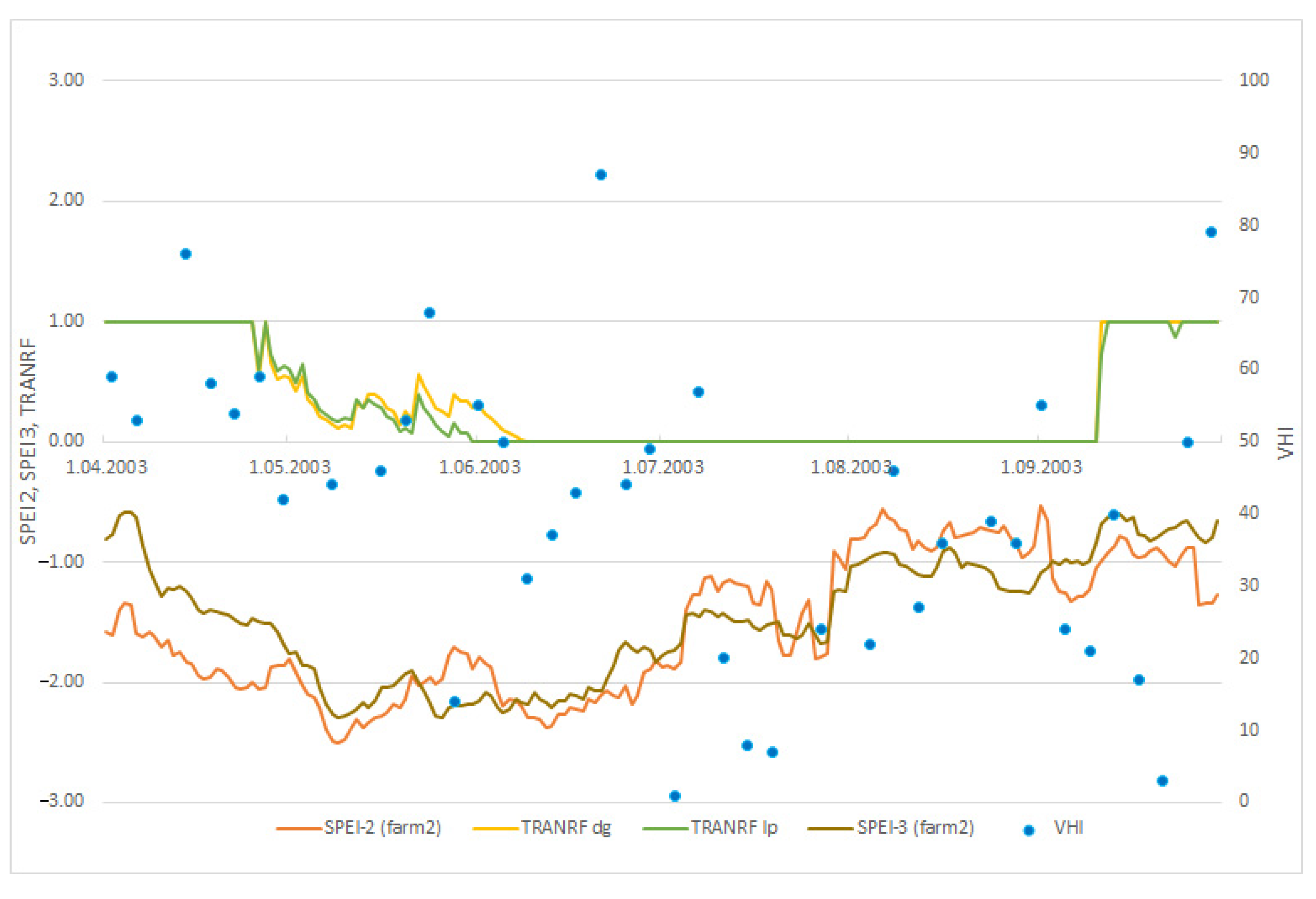
For 2003 (Figure 9), the comparison was similar to that for 2013, which was due to the prolonged drought in both years. The agreement between the model and satellite data indices was best for early summer from early May to mid-June, with a decreasing trend in both SPEI-2 and SPEI-3 and a local maximum in early June. Although the trends of SPEI-2 and SPEI-3 increased slightly from mid-June to early September, we could not find anything comparable in the TRANRF time series. Conversely, the VHI time series showed that the values fell below 40 (upper limit for drought) in early July and then remained in the interval around 10–20 (significant drought) until early September, when the TRANRF value has already risen to the maximum.
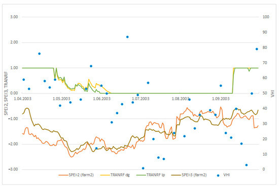
Figure 9.
Time series of the LINGRA-N model results of drought factor (TRANRF) using the parameter set calibrated for Dactylis glomerata in Jablje (dg) and Lolium perenne in Jablje (lp); time series of drought indices (VHI, SPEI-2 and SPEI-3) for Farm2, all for 2003.
Comparison of SPEI-2 and SPEI-3 Indices with TRANRF, SMACT, WRE, and WRT
As mentioned in the beginning of the previous chapter, we again took into account only the years of data with high drought impact, with the purpose being to emphasise only the impact of drought and not the impact of other factors on the drought evaluation. The best regression model results using the coefficient of determination (r2) for SPEI-3 compared to the model results (Table 3) were found for SMACT for the lp calibration on Farm1i, with the statistically significant value of 0.346 (p < 0.001), indicating that approximately 35% of the variability in SMACT is explained by SPEI-3. Another model drought indicator for which the linear regression model was calculated is WRT, with the highest r2 between WRT and SPEI-3 with the statistically significant value of 0.137 (p < 0.001).
Table 3.
Statistical analysis of drought index SPEI-3 at Farms1e and 1i and the LINGRA-N model results of yield (TRANRF, SMACT, WRE, WRT) for year 2017—shown are values of r2.
The results of the linear regression model for 2013 and 2003 for Farm2 and the same combination of indices (Table 4) had the highest values of r2 for the indices WRT and SPEI-3 in 2013: for dg is r2 = 0.868 (p < 0.001), and for lp is r2 = 0.809 (p < 0.001). Very high values of r2 were also found for SMACT using lp calibration, namely r2 = 0.735 (p < 0.001), which means that about 74% of the variability in SMACT is explained by the SPEI-3 index.
Table 4.
Statistical analysis of drought index SPEI-3 at Farm2 and the LINGRA-N model results of yield (TRANRF, SMACT, WRE, WRT) for years 2013 and 2003—shown are values of r2.
For SPEI-2 at higher elevation farms, the highest but relatively low values of the coefficient of determination were calculated for the comparison to SMACT for the lp calibration in 2017 (Table 5) with the value of r2 = 0.268 (p < 0.001). The results for 2013 for Farm2 (Table 6) were significantly better than the results for 2017 and 2003. The value of r2 was the highest for the combination of SPEI-2 and SMACT for 2013, which was r2 = 0.724 (p < 0.001).
Table 5.
Statistical analysis of drought index SPEI-2 at Farms1e and 1i and the LINGRA-N model results of yield (TRANRF, SMACT, WRE, WRT) for year 2017—shown are values of r2.
Table 6.
Statistical analysis of drought index SPEI-2 at Farm2 and the LINGRA-N model results of yield (TRANRF, SMACT, WRE, WRT) for years 2013 and 2003—shown are values of r2.
A high value of r2 was also found for TRANRF, namely, for both grass species, the value of r2 was greater than or equal to 0.6 (r2 = 0.600; p < 0.001 for dg, r2 = 0.667; p < 0.001 for lp). Nevertheless, the graphical representation (not shown) showed that the fit of the linear regression line to the data is not reliable due to the outliers (TRANRF = 0 and TRANRF = 1), which distort the result.
4. Discussion
The major advantage of models such as LINGRA [39] is that they can be used under different weather and soil conditions, in different environments, and in different regions of the world [40]. Due to weather influences, grassland areas show a pronounced annual variability [41] and it is important that livestock farms in Europe take this risk into account [42]. There is still a gap between what stakeholders in the agricultural sector need in terms of spatial resolution and the meteorological drought information available from observations or models [43], which is why remote sensing is also important to be included as much as possible.
Species responses to drought are not the same. Usually, dg tolerates drought better, while lp tolerates drought less well and sometimes even perishes. From the model-field yield comparison on annual basis, the best calibration option was chosen for further use of the daily modelled data. Several advances have been made in the last two decades in the development of drought indices using remote sensing [44], but the relationships between drought indices and agricultural drought impacts vary across Europe [45]. Given the recommended usage of the “extreme” years to determine which drought index should be selected for monitoring agricultural drought conditions [19], we focused on 2003, 2013, and 2017.
While SPEI-2 in 2017 better reflected the TRANRF maximum in early June than SPEI-3, the trend in SPEI-3 showed greater agreement with the trend in TRANRF. This is largely due to the nature of the SPEI-2 index, which contains more data than its smoothed version, the SPEI-3 index. In 2003, the value of TRANRF was 0 for a very long time, but SPEI increased slightly toward the end of the summer. A possible explanation could be that in the model, transpiration stopped completely for the plant and started again only when the drought ended permanently. However, both SPEI-2 and SPEI-3 indices were strongly correlated with the model variables TRANRF, SMACT, and WRT, with r2 higher than 0.5 and statistically significant in the lower elevation Farm2 in 2013, but not in the two higher elevation farms in 2017. The reason may also be a very short period of data in the higher elevation farms. The correlation was also poor in 2003 when the link between the model and the field data was also not so good. To monitor agricultural drought in the south and central U.S., research showed that SPEI best reflects soil moisture [19]. At the pan-European scale, short accumulation periods of SPEI are best associated with plant vegetation stress in most cases. For Europe as a whole, SPEI-3 and SPEI-4 in particular are well associated with vegetation conditions [45]. SPEI is also designed to capture climatic conditions that may cause drought occurrence, but topography is an important factor affecting its ability [44].
VHI has the potential to detect agricultural and vegetation-based drought, respectively, from both soil and vegetation-based perspectives [46]. In China, the overall performance of VHI in capturing soil moisture dynamics was relatively poor and subject to many uncertainties [47], but in Bavaria, Germany, VHI correlated well with soil moisture and yield data, especially in the summer months of July and August on agricultural land and grassland below 800 m, where water is the primary limiting factor for plant growth [46]. In the Slovenian Alpine region, it mainly follows the TRANRF and SPEI trajectories, but should probably not be the only one to use. Like others [19], we would like to emphasise that no single drought index can capture all aspects of agricultural drought.
Regardless of the purpose of using the agricultural drought index, the decision of which index to choose has a major impact on the accuracy of the information, which varies by crop, region, and spatial scale [48]. Remote sensing data based on vegetation condition provide a better picture of local drought conditions than drought indices based only on rainfall [19], so we recommend a combination of indices and modelling, or at least their evaluation.
A limitation of the study is that the original LINGRA-N model is a simplification of reality, as all models are. It was developed to simulate the growth of frequently mowed and intensively managed grassland, as occurs in the Netherlands [49], and it was not additionally calibrated (but previously calibrated version for another part of Slovenia was used). When data are available, we recommend a new calibration of the model, especially also by using other measurements that include not only yield (e.g., LAI). In addition, the inclination of the fields cannot be taken into account in the model. Crop yield is also affected by more than just moisture conditions, and below average yield is not necessarily indicative of dry conditions, but can be affected by other factors such as disease, pests, fertility, and cropping practices [19]. We made assumptions about the relationship between drought and yield or growth parameters, but tried to use several model variables to exclude other options as much as possible. Finally, crop models and drought indices rely to some extent on the same weather inputs, and this creates a kind of collinearity issue that can bias the results. The results of this study are specific to a case study in the Alpine region, but the method and results can be applied to other regions to determine the optimal drought indices for monitoring agricultural drought conditions.
5. Conclusions
The model results of annual grassland yield for three farms agreed well with the estimated yields in the lower part of the Slovenian Alpine region, with lower yields in the extremely dry year 2003 and in the dry years 2007, 2013 and 2017. LINGRA-N well described regrowth after defoliation (mowing), leaf area development stopped in lp after the fourth mowing, and after each mowing, the difference between lp and dg continued to increase. A time series comparison of the LINGRA-N results using the calibration for dg and lp and the drought indices VHI, SPEI-2, and SPEI-3 was performed for the dry years 2003, 2013, and 2017 to observe the correlation of the indices under the most significant drought conditions. Evaluation of the drought indices SPEI-2 and SPEI-3 showed that both indices were strongly correlated with the model variables TRANRF (drought factor), SMACT (actual root zone water content), and WRT (root dry weight). The VHI index also captured good local minima in the modelled TRANRF. All correlation between indices and the most drought-responsive modelled variables implies that the drought conditions were also well captured by the indices. The agreement between SPEI and TRANRF depends on the length and intensity of the drought. SPEI-2, which contains more data than its smoothed version, SPEI-3, better reflects the maximum of TRANRF during short-term drought events. Based on our case study, we recommend the inclusion of a variety of drought indices and a modelling approach to agricultural drought monitoring, as the combination of field measurement data, modelled data, and remote sensing data can greatly improve drought management practices.
Author Contributions
Conceptualisation, T.P. and A.S.; Methodology, T.P.; Validation, T.P. and Z.Ž.; Formal analysis, Z.Ž.; Resources, Ž.V. and Z.Č.; Writing—original draft preparation, T.P., Z.Ž. and Ž.V.; Writing—review and editing, Z.Č. and A.S.; Visualisation, Z.Ž.; Supervision, A.S.; Project administration, Ž.V.; Funding acquisition, A.S.; Contextualisation, Ž.V.; Project administration, Ž.V. All authors have read and agreed to the published version of the manuscript.
Funding
This paper was produced within the Alpine Drought Observatory (ADO) project, which was funded by the Alpine Space Programme (2018–2021).
Institutional Review Board Statement
Not applicable.
Informed Consent Statement
Not applicable.
Data Availability Statement
Not applicable.
Conflicts of Interest
The authors declare no conflict of interest. The funders had no role in the design of the study; in the collection, analyses, or interpretation of data; in the writing of the manuscript, or in the decision to publish the results.
References
- Cammalleri, C.; Naumann, G.; Mentaschi, L.; Formetta, G.; Forzieri, G.; Gosling, S.; Bisselink, B.; De Roo, A.; Feyen, L. Global Warming and Drought Impacts in the EU; Publications Office of the European Union: Luxembourg, 2020; Available online: https://ec.europa.eu/jrc/sites/jrcsh/files/pesetaiv_task_7_drought_final_report.pdf (accessed on 7 July 2021).
- Spinoni, J.; Naumann, G.; Barbosa, P.; Vogt, J. Meteorological Droughts in Europe: Events and Impacts, Past Trends and Future Projections; Publications Office of the European Union: Luxembourg, 2016; Available online: https://data.europa.eu/doi/10.2788/450449 (accessed on 2 December 2021).
- Sušnik, A.; Gregorič, G. Kmetijska suša v 21. Stoletju v Sloveniji. 28. Mišičev Vodarski Dan 2017. 2017. Available online: http://www.mvd20.com/LETO2017/R5.pdf (accessed on 3 November 2021).
- García-Herrera, R.; Díaz, J.; Trigo, R.M.; Luterbacher, J.; Fischer, E.M. A Review of the European Summer Heat Wave of 2003. Crit. Rev. Environ. Sci. Technol. 2010, 40, 267–306. [Google Scholar] [CrossRef]
- Stephan, R.; Erfurt, M.; Terzi, S.; Žun, M.; Kristan, B.; Haslinger, K.; Stahl, K. An inventory of Alpine drought impact reports to explore past droughts in a mountain region. Nat. Hazards Earth Syst. Sci. 2021, 21, 2485–2501. [Google Scholar] [CrossRef]
- Mastrotheodoros, T.; Pappas, C.; Molnar, P.; Burlando, P.; Manoli, G.; Parajka, J.; Rigon, R.; Szeles, B.; Bottazzi, M.; Hadjidoukas, P.; et al. More green and less blue water in the Alps during warmer summers. Nat. Clim. Chang. 2020, 10, 155–161. [Google Scholar] [CrossRef]
- Haslinger, K.; Schöner, W.; Anders, I. Future drought probabilities in the Greater Alpine Region based on COSMO-CLM experiments—Spatial patterns and driving forces. Meteorol. Z. 2015, 25, 137–148. [Google Scholar] [CrossRef]
- Calanca, P. Climate change and drought occurrence in the Alpine region: How severe are becoming the extremes? Glob. Planet. Chang. 2007, 57, 151–160. [Google Scholar] [CrossRef]
- EEA. The Alpine Region—Biodiversity, Energy and Water—European Environment Agency. 2020. Available online: https://www.eea.europa.eu/themes/regions/the-alpine-region/biodiversity-energy-water/biodiversity-energy-and-water (accessed on 6 November 2021).
- Rosbakh, S.; Leingärtner, A.; Hoiss, B.; Krauss, J.; Steffan-Dewenter, I.; Poschlod, P. Contrasting Effects of Extreme Drought and Snowmelt Patterns on Mountain Plants along an Elevation Gradient. Front. Plant Sci. 2017, 8, 1478. Available online: https://www.frontiersin.org/article/10.3389/fpls.2017.01478 (accessed on 17 November 2021). [CrossRef] [PubMed] [Green Version]
- Larcher, W. Physiological Plant Ecology, 4th ed.; Springer: Berlin/Heidelberg, Germany, 2003; Available online: https://link.springer.com/book/9783540435167 (accessed on 7 March 2022).
- Jäger, H.; Peratoner, G.; Tappeiner, U.; Tasser, E. Grassland biomass balance in the European Alps: Current and future ecosystem service perspectives. Ecosyst. Serv. 2020, 45, 101163. [Google Scholar] [CrossRef]
- Labadini, A.; Candiago, S.; Egarter Vigl, L.; Marsoner, T.; Tasser, E.; Roilo, S.; Romelli, C.; Carloni, R.; Pecher, C.; Summer, H.; et al. Ecosystem Services and Governance in the Alps: Tools and Tips for Effective Environmental Management and Territorial Development; Eurac Research: Bolzano, Italy, 2019; Available online: https://hdl.handle.net/10863/12097 (accessed on 19 November 2021).
- EEA. The Alpine Region—European Environment Agency. 2008. Available online: https://www.eea.europa.eu/publications/report_2002_0524_154909/biogeographical-regions-in-europe/alpine.pdf/view (accessed on 7 November 2021).
- Schucknecht, A.; Krämer, A.; Asam, S.; Mejia-Aguilar, A.; Garcia-Franco, N.; Schuchardt, M.A.; Jentsch, A.; Kiese, R. Vegetation traits of pre-Alpine grasslands in southern Germany. Sci. Data 2020, 7, 316. [Google Scholar] [CrossRef]
- Slovenian Environment Agency (ARSO). Report on Existing Monitoring Platforms and Potential Data for the Integration into ADO. 2020. Available online: https://www.alpine-space.org/projects/ado/d.t.1.1.2/dt1.1.2_regional-report_drought-monitoring.pdf (accessed on 7 November 2021).
- World Meteorological Organization (WMO) and Global Water Partnership (GWP). Handbook of Drought Indicators and Indices (M. Svoboda & B.A. Fuchs). Integrated Drought Management Programme (IDMP), Integrated Drought Management Tools and Guidelines Series 2. 2016. Available online: https://www.droughtmanagement.info/literature/GWP_Handbook_of_Drought_Indicators_and_Indices_2016.pdf (accessed on 7 December 2021).
- Bhuyan-Erhardt, U.; Erhardt, T.; Laaha, G.; Parajka, J.; Zang, C.; Menzel, A. Validation of drought indices using environmental indicators: Streamflow and carbon flux data. Agric. For. Meteorol. 2019, 265, 218–226. [Google Scholar] [CrossRef]
- Kloos, S.; Yuan, Y.; Castelli, M.; Menzel, A. Agricultural Drought Detection with MODIS Based Vegetation Health Indices in Southeast Germany. Remote Sens. 2021, 13, 3907. [Google Scholar] [CrossRef]
- Zeng, J.; Zhang, R.; Qu, Y.; Bento, V.A.; Zhou, T.; Lin, Y.; Wu, X.; Qi, J.; Shui, W.; Wang, Q. Improving the drought monitoring capability of VHI at the global scale via ensemble indices for various vegetation types from 2001 to 2018. Weather Clim. Extrem. 2022, 35, 100412. [Google Scholar] [CrossRef]
- Bowell, A.; Salakpi, E.E.; Guigma, K.; Muthoka, J.M.; Mwangi, J.; Rowhani, P. Validating commonly used drought indicators in Kenya. Environ. Res. Lett. 2021, 16, 084066. [Google Scholar] [CrossRef]
- Kozjek, K. Objektivna Opredelitev Podnebnih Regij Slovenije, Magistrsko Delo; Faculty of Mathematics and Physics, University of Ljubljana: Ljubljana, Slovenia, 2016; Available online: https://repozitorij.uni-lj.si/Dokument.php?id=106356&lang=slv (accessed on 3 March 2022).
- Bouman, B.; Schapendonk, A.; Stol, W.; Kraalingen, D.W.G. Description of the Growth Model LINGRA as Implemented in CGMS. Quantitative Approaches in Systems Analysis No. 7; AB-DLO: Wageningen, The Netherlands, 1996. [Google Scholar]
- Schapendonk, A.H.C.M.; Stol, W.; van Kraalingen, D.W.G.; Bouman, B.A.M. LINGRA, a sink/source model to simulate grassland productivity in Europe. Eur. J. Agron. 1998, 9, 87–100. [Google Scholar] [CrossRef]
- Diepen, C.A.; Boogaard, H.L.; Supit, I.; LAZAR, C.; Orlandi, S.; van der Goot, E.; Schapendonk, A. Methodology of the MARS Crop Yield Forecasting System. Vol. 2 Agrometeorological Data Collection, Processing and Analysis; DG JRC IPSC: Ispra, Italy, 2004. [Google Scholar]
- Wolf, J. User Guide for LINGRA-N: Simple Generic Model for Simulation of Grass Growth under Potential, Water Limited and Nitrogen Limited Conditions; Wageningen University: Wageningen, The Netherlands, 2012; Available online: https://www.wur.nl/en/Publication-details.htm?publicationId=publication-way-343434373232 (accessed on 28 March 2013).
- Pogačar, T.; Bogataj, L.K. Simulation of grass sward dry matter yield in Slovenia using the LINGRA-N model. Ital. J. Agron. 2018, 13, 44–56. [Google Scholar] [CrossRef] [Green Version]
- Slovenian Environment Agency (ARSO). 2021; Meteorological Data Archive. Available online: http://meteo.arso.gov.si/met/sl/archive (accessed on 5 September 2021).
- Huang, J. A Simple Accurate Formula for Calculating Saturation Vapor Pressure of Water and Ice. J. Appl. Meteorol. Climatol. 2018, 57, 1265–1272. [Google Scholar] [CrossRef]
- Vicente-Serrano, S.M.; Beguería, S.; López-Moreno, J.I. A Multiscalar Drought Index Sensitive to Global Warming: The Standardized Precipitation Evapotranspiration Index. J. Clim. 2010, 23, 1696–1718. [Google Scholar] [CrossRef] [Green Version]
- McKee, T.B.; Doesken, N.J.; Kleist, J. The Relationship of Drought Frequency and Duration to Time Scales; Dept. of Atmos Sci, Fort Collins University: Fort Colins, Colorado, 1993. [Google Scholar]
- Stagge, J.H.; Tallaksen, L.M.; Gudmundsson, L.; Van Loon, A.F.; Stahl, K. Candidate Distributions for Climatological Drought Indices (SPI and SPEI). Int. J. Climatol. 2015, 35, 4027–4040. [Google Scholar] [CrossRef]
- Hersbach, H.; Bell, B.; Berrisford, P.; Biavati, G.; Horányi, A.; Muñoz Sabater, J.; Nicolas, J.; Peubey, C.; Radu, R.; Rozum, I.; et al. ERA5 Hourly Data on Single Levels from 1979 to Present; Copernicus Climate Change Service (C3S); Climate Data Store (CDS): Reading, UK, 2018. [Google Scholar] [CrossRef]
- Bazile, E.; Abida, R.; Szczypta, C.; Verelle, A.; Soci, C.; LeMoigne, P. Project: 607193 UERRA, Deliverable D2.9: Ensemble Surface Reanalysis Report. 2017. Available online: https://www.uerra.eu/component/dpattachments/?task=attachment.download&id=283 (accessed on 23 November 2021).
- Kogan, F.N. Application of vegetation index and brightness temperature for drought detection. Adv. Space Res. 1995, 15, 91–100. [Google Scholar] [CrossRef]
- Kogan, F.N. Global Drought Watch from Space. Bull. Am. Meteorol. Soc. 1997, 78, 621–636. [Google Scholar] [CrossRef]
- Vermote, E.; Wolfe, R. MOD09GQ MODIS/Terra Surface Reflectance Daily L2G Global 250m SIN Grid V006 [Dataset]; NASA EOSDIS Land Processes DAAC: Sioux Falls, SD, USA, 2015. [Google Scholar] [CrossRef]
- Wan, Z.; Hook, S.; Hulley, G. MOD11A1 MODIS/Terra Land Surface Temperature/Emissivity Daily L3 Global 1km SIN Grid V006 [Dataset]; NASA EOSDIS Land Processes DAAC: Sioux Falls, SD, USA, 2015. [Google Scholar] [CrossRef]
- Barrett, P.D.; Laidlaw, A.S. Utilisation of Grazed Grass in Temperate Animal Systems; Murphy, J.J., Ed.; Wageningen Academic Publishers: Wageningen, The Netherlands, 2005. [Google Scholar] [CrossRef]
- Žalud, Z.; Trnka, M.; Ruget, F.; Hlavinka, P.; Eitzinger, J.; Schaumberger, A. Evaluation of Crop Model STICS in the Conditions of the Czech Republic and Austria; Sbornik Strecno: Strecno, Czech Republic, 2006. [Google Scholar]
- Herrmann, A.; Kelm, M.; Kornher, A.; Taube, F. Performance of grassland under different cutting regimes as affected by sward composition, nitrogen input, soil conditions and weather—A simulation study. Eur. J. Agron. 2005, 22, 141–158. [Google Scholar] [CrossRef]
- Trnka, M.; Eitzinger, J.; Gruszczynski, G.; Buchgraber, K.; Resch, R.; Schaumberger, A. A simple statistical model for predicting herbage production from permanent grassland. Grass Forage Sci. 2006, 61, 253–271. [Google Scholar] [CrossRef]
- García-León, D.; Contreras, S.; Hunink, J. Comparison of meteorological and satellite-based drought indices as yield predictors of Spanish cereals. Agric. Water Manag. 2019, 213, 388–396. [Google Scholar] [CrossRef]
- Lawal, S.; Hewitson, B.; Egbebiyi, T.S.; Adesuyi, A. On the suitability of using vegetation indices to monitor the response of Africa’s terrestrial ecoregions to drought. Sci. Total Environ. 2021, 792, 148282. [Google Scholar] [CrossRef] [PubMed]
- Bachmair, S.; Tanguy, M.; Hannaford, J.; Stahl, K. How well do meteorological indicators represent agricultural and forest drought across Europe? Environ. Res. Lett. 2018, 13, 034042. [Google Scholar] [CrossRef]
- Liu, Q.; Zhang, J.; Zhang, H.; Yao, F.; Bai, Y.; Zhang, S.; Meng, X.; Liu, Q. Evaluating the performance of eight drought indices for capturing soil moisture dynamics in various vegetation regions over China. Sci. Total Environ. 2021, 789, 147803. [Google Scholar] [CrossRef] [PubMed]
- Tian, L.; Yuan, S.; Quiring, S. Evaluation of six indices for monitoring agricultural drought in the south-central United States. Agric. For. Meteorol. 2018, 249, 107–119. [Google Scholar] [CrossRef]
- Quiring, S.M.; Papakryiakou, T.N. An evaluation of agricultural drought indices for the Canadian prairies. Agric. For. Meteorol. 2003, 118, 49–62. [Google Scholar] [CrossRef]
- Giannitsopoulos, M.L.; Burgess, P.J.; Richter, G.M.; Bell, M.J.; Topp, C.F.E.; Ingram, J.; Takahashi, T. Modelling the Interactions of Soils, Climate, and Management for Grass Production in England and Wales. Agronomy 2021, 11, 677. [Google Scholar] [CrossRef]


Publisher’s Note: MDPI stays neutral with regard to jurisdictional claims in published maps and institutional affiliations. |
© 2022 by the authors. Licensee MDPI, Basel, Switzerland. This article is an open access article distributed under the terms and conditions of the Creative Commons Attribution (CC BY) license (https://creativecommons.org/licenses/by/4.0/).