A Case Study in Desertified Area: Soybean Growth Responses to Soil Structure and Biochar Addition Integrating Ridge Regression Models

Abstract

Desertified land covers one-fourth of the world’s total land area. Meeting the high food demands in areas affected by desertification is a major problem. This case study provided fundamental information to demonstrate the potential for utilizing the desertified land. The soybean trial was established in two sandy clay loam soils (desertified land) and one silty clay loam soil. Two types of biochar were applied as treatments. We aimed to investigate the response of soybean plants to soil structure, soil nutrient condition, and biochar amendment in the two types of soil. In addition, ridge regression was employed to model the plant growth indicators by soil structure, soil nutrients condition, soil water content, and biochar amendment. We conclude that (1) overall soil productivity in sandy clay loam soil is lower than in silty clay loam soil. The sandy clay loam soil may have high efficacy for crop production due to its higher harvest index. (2) Aggregate size 0.5–1 mm, 1–2 mm, and 2–3 mm indicated more important in plant biomass formation in silty clay loam soil. The low aggregate stability of sandy clay loam soil made the field more vulnerable to wind erosion in the semi-arid monsoon climate. (3) Cob biochar and wood biochar increased soybean shoot biomass by 48.7% and 45.0% in silty clay loam soil. (4) The higher N-fixing ability of nodules in sandy clay loam soil indicates an advantage to reduce the use of N-fertilizers in desertified areas. (5) Exponential polynomial regression ameliorated the accuracy of prediction of plant growth indicators in comparison to linear regression.

1. Introduction

Desertified land occupies 3.6 × 10⁷ km², approximately 30% of the total land area in the world [1]. Three billion of the world’s population are affected by desertification and land degradation [2]. To combat desertification, an effective measure, “farmland shelterbelt network”, was pointed out by Long (2019) [1]. The farmlands combined with the shelterbelt network may increase agricultural harvests and improve economic growth [1]. This measure considered both nature of local community development and desertification techniques for sustainable desertification prevention.

In this case study, the investigated cropping fields are in front of the Tengger Desert in northwestern China (Figure 1). The edge area of the region was desertified and thus featured low water and nutrient-holding capacity. The land in the region was fallow before 1995, and the situation conversed with the local economy growth and farming system development until 1995. Nowadays, the local community invests in cropping in this area by overusing chemical fertilizer and irrigation to gain profit. Therefore, sustainably establishing a cropping system is critical for both productivity and agro-ecosystem health. A systematic investigation of soil physical structure, soil chemical properties, and soil amendment is needed to sustain the efficacy of crop production in the desertified area.

As a source of protein and oil, soybeans are produced in many countries and contribute about 67% of the world’s protein meal supply [3,4]. Additionally, the biological nitrogen fixation of soybean nodules can produce as much as 450 kg ha⁻¹ of nitrogen [5]. Leghemoglobin (Lb) takes 40% of all nodule protein and plays important role in N fixation. Lb supports the energy metabolism through its O₂-binding heme group in nodules for the demand of the symbiont N fixation [6]. Thus, Lb content is an important indicator of N-fixation activity. Soybean cropping in desertified land may provide a sustainable N source to relieve the overusing of N fertilizer.

Soil structure plays important role in soil fertility and agricultural productivity. It affects soil water transportation, plant seed germination, and microbial activity [7,8]. Aggregation is a crucial soil function for maintaining soil porosity and enhancing the stability of soil structure [9,10]. Soil aggregation forms from the rearrangement of particles by flocculation and cementation. Therefore, its abundance may indicate soil stability. Dry aggregate size distribution (ASD) is one of the major physical characteristics of soil, which affects soil fertility and stability. The aggregate fraction of 0.25–10 mm is considered a soil quality indicator since it determines soil water and air capacity [11,12]. Dry mean weight diameter (MWD) is a common index of dry ASD for evaluating soil aggregate stability. Higher MWD represents higher water permeability and air capacity in soil [11,13]. Soil aggregation may also be indicated by dry geometric mean diameter (GMD). Due to a strong correlation to soil erodible fraction, the GMD can be used as a predictor of wind erosion [14].

Organic matter has been reported to have positive effects on enhancing soil aggregation [15,16]. Biochar, as a kind of organic matter, is capable of enhancing soil structures and fertility qualities [17,18]. It presents in small clusters of soil particles or soil aggregates associated with the fine soil fraction (50 µm) [19,20,21,22]. Therefore, biochar can be a binding agent for organic matter in aggregate formation and thus alleviate aggregates degradation and strengthen soil stability [19,22]. Nevertheless, the effects of biochar on soil properties depend on many factors, such as the feedstock, pyrolysis process, and soil types. The biochar was also reported to not affect soil aggregation [23,24,25]. The specific mechanism of biochar’s effect on soil water retention, soil aggregation, soil stability, and their interrelationship with plant growth still needs to be well-demonstrated [26,27,28,29].

Further, by integrating soil structure, soil chemical properties, and biochar amendment, crop modeling may provide a reference cropping pattern from this field study to other desertified areas. Machine learning enables model prediction in multivariate and intricate datasets [30]. To avoid overfitting the model, the data usually are separated into train and test sets. The train set is used to compute a model parameter, and the test set validates the training result, tunes the model hyperparameters, and evaluates the generalization error [30]. The ridge regression model is employed in machine learning to solve problems in the estimation of models with correlated predictors [31,32]. Additionally, ridge regression is also used to overcome the parameter estimates fluctuation caused by multicollinearity [33]. The multicollinearity is a challenge for establishing a reliable crop model, especially in this multivariate study. Thus, it is appropriate to use ridge regression to predict crop growth indicators in this study.

The objectives of this study are to (a) investigate the response of soybean plants to the soil structure, soil nutrient condition, and biochar amendment in sandy clay loam soil (desertified land) and silty clay loam soil; (b) elucidate the interrelationship among soybean growth, soil structure, nitrogen fixation ability of nodule, and biochar; and (c) predict the soybean growth indicators by soil nutrients, soil aggregate sizes, soil water content, and biochar amendment by employing the ridge regression models.

2. Materials and Methods

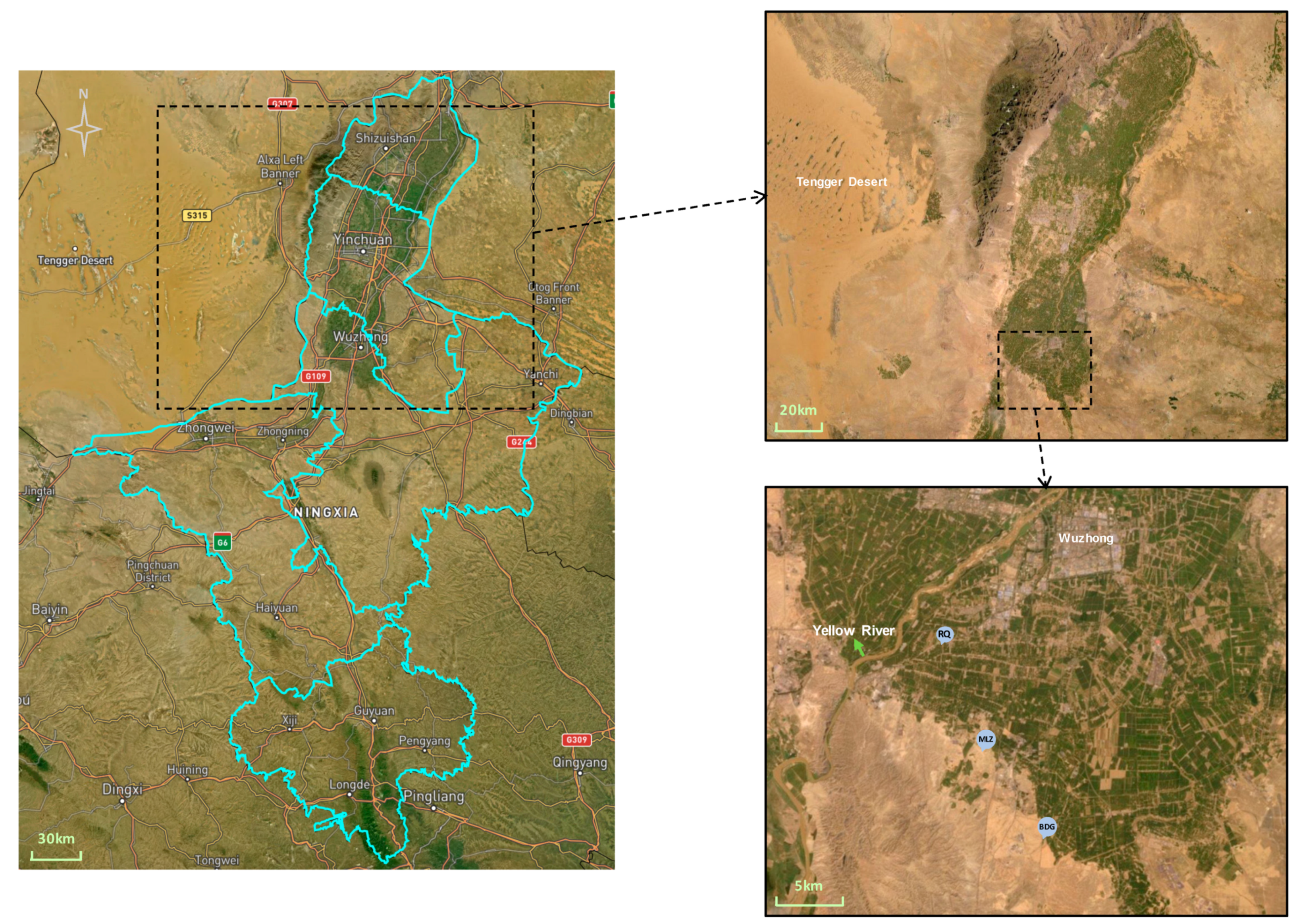
2.1. Study Site and Field Design

Soybean trials were performed on two sandy clay loam fields (desertified) and one silty clay loam field at three villages in Wuzhong city, Ningxia Hui Autonomous Region, China. The two sandy clay loam fields were located at Biandangou (BDG, 37.78840° N, 106.18311° E) and Miaoliangzi (MLZ, 37.85167° N, 106.11749° E) villages at the edge of the investigated region. The silty clay loam field was located at Renqiao (RQ, 37.91330° N, 106.07423° E) village in the vegetation-covered area. The study area is exposed to the Tengger Desert, which occupies 36,700 km² of land, and the distance to the desert is as close as 60 km (Figure 1). Therefore, these two sandy clay loam fields at the edge of the region are desertified fields. The soil texture in the three fields was characterized by sand, silt, and clay content as 45.4, 19.5, and 34.5% for BDG; 41.5, 23.8, and 32.6% for MLZ, and 4.1, 50.7, and 37.5% for RQ, respectively. The region is characterized as a semi-arid, temperate, continental monsoon climate. In 2016, the annual precipitation and evaporation evapotranspiration were 289.3 mm and 1297.7 mm, respectively. The average temperature was 10.2°C in the whole year and the annual sunshine hours was 3230.1. It was often windy from June to October and accompanied by wind erosion; the maximum wind velocity reached 10.7 m s⁻¹ m, and the annual mean wind velocity was 1.8 m s⁻¹. The average temperature was 23.8 °C, and the precipitation was 80.5 mm in the Wuzhong area during the cropping season from 17 May to 12 October. The sandy clay loam fields were irrigated two times per month, whereas the silty clay loam field was irrigated one time per month. Each field was divided into seven groups representing seven replications. Each replication group consisted of two treatments and control, i.e., (a) 20 t ha⁻¹ cob biochar (CB) application, (b) 20 t ha⁻¹ wood biochar (WB) application, and (c) without biochar (CK) application. The treatments and control were randomly distributed in each replication. Each treatment or control was represented by a plot in the field, and the plot size was 5 m by 2 m. Equivalent amounts of 50 and 60 kg ha⁻¹ of phosphorus and potassium fertilizer were applied in silty clay loam soil, while 60, 100, and 120 kg ha⁻¹ of equivalent nitrogen, phosphorus, and potassium fertilizer were applied in two sandy clay loam soils. The biochar used in the field study was produced at 450 °C from mixed wood (poplar and apple tree) and maize cob, with a particle size of less than 2 mm (

Table 1. Biochar characteristics.

Biochar Feedstock	Total (g kg−1)		Available (mg kg−1)		C/N
	C	N	K	P
Mixed wood	712	7.53	2698	191	95
Maize cob	755	5.1	3802	65	148

). The biochar was mixed with a cultivator at 15 cm depth before sowing. Then, soybean seeds (Glycine max L. var. Zhong Huang) were sown with a 35 cm row interval in each plot.

2.2. Plant Sampling and Analysis

At 90 days after planting, four spots were sampled in each plot; the plants in 15 cm width and 15 cm length of the area at each spot were sampled for plant biomass analysis. For plant sampling, the whole plant was carefully dug up at a depth of 25 cm, and then, the root system was rinsed carefully, and the nodules were removed. After plant sampling, shoots were separated from roots for measurements of plant dry weight. All plant materials were dried in an oven at 68 °C for 48 h; then, the dry weight was determined. At 120 days after planting, the plants were sampled in the same way for grain yield determination. Then, soybean seeds were removed from pods and dried for grain yield determination. After the dry weight was determined, the plant and grain materials were ground using a mill fitted with a 1 mm screen; then, they were sub-sampled for the analysis of plant total C (TC), total N (TN), phosphorus (P), potassium (K), and magnesium (Mg) concentrations. The N, P, and K concentrations in plant tissue were analyzed with an inductively coupled plasma optical emission spectrometer (ICP-OES; iCAP 6300 Duo). Harvest index (HI) is calculated as:

HI = grain yield/total biomass

2.3. Nodule Sampling and Leghemoglobin Content Analysis

Nodules were carefully collected from the roots after rinsing with water. The Lb content determination used the method by Ma et al. [34]. The nodules were ground, and 0.5 mg subsample was taken and mixed with 3 mL of Drabkin’s solution for Lb extraction. The mixture was centrifuged at 500× g for 15 min, and the supernatant was moved to a 10 mL tube. The Lb extraction was repeated twice with left ground nodules, and the supernatants were combined. The volume of combined supernatants was adjusted to 10 mL with Drabkin’s solution. Afterward, the combined supernatants were centrifuged at 20,000× g for 30 min. The Lb content was standardized with a solution of bovine hemoglobin.

2.4. Soil Sampling and Physicochemical Properties Analysis

After the last plant sampling, soil samples were taken for soil moisture, nutrients concentration, and aggregate structure analysis, i.e., (a) for the soil moisture analysis, the soil samples were taken by a core cutter with the 5 × 5 cm of height and diameter at the soil depth of 10–15 cm. The weight of the soil was immediately measured. Subsequently, the soil was dried at 105 °C to reach a constant weight; (b) for the soil nutrients concentration determination, the soil was sampled by a shovel at the depth of 10–15 cm. The TC, TN, and total sulfur (TS) contents of soil samples were determined by the dry combustion method [35] using an elemental determinator (TruSpec CNS). P, K, Mg, and calcium (Ca) were analyzed with an ICP-OES (iCAP 6300 Duo) via the method Mehlich-3 extraction, while (c) for the soil aggregate structure analysis, two spots in each plot were selected for soil sampling; the soil was taken by shovel carefully at the depth of 15 cm to avoid a damage of the soil structure. Then, 300 g of the collected soil samples were grouped by 0.25, 0.5, 1, 2, 3, 5, 7, and 10 mm sieves. Therefore, nine aggregate size classes (ASCs) were obtained (>10, 10–7, 7–5, 5–3, 3–2, 2–1, 1–0.5, 0.5–0.25, and <0.25 mm). Dry ASD was determined by the standard dry-sieving method [11].

Using the weights of these ASCs, MWD (mm) is calculated [36]:

$$\mathrm{MWD}={\displaystyle \sum }_{i=1}^n{x}_i{w}_i$$

where w_i is the weight percentage of each aggregate size class to the total sample, and x_i is the mean diameter of each aggregate size class (mm).

Dry GMD (mm) is calculated as [36]:

$$\mathrm{GMD}=\exp \left[{\displaystyle \sum }_{i=1}^n\frac{(w_i\log \left(x_i\right))}{w_1}\right]$$

where w_i is the weight percentage of each aggregate size class to the total sample, and x_i is the mean diameter of each aggregate size class (mm).

2.5. Ridge Regression Model

Ridge regression may overcome problems of multicollinearity in standard ordinary least square (OLS) regression [37]. The ridge regression model is also employed in machine learning to solve problems in the estimation of models with correlated predictors [38,39].

In usual multiple linear regression:

Y = β₀ + β₁X₁ + β₂X₂ + …+ β_pX_p + ε

where Y represents the response variable, X_j represents the predictor variable, β_j represents the average effect on Y of a one unit increase in X_j, and ε refers to the error term.

The OLS estimator minimizes the residual sum of squares (RSS):

$$\mathrm{RSS}={\sum }_i{(y_i-{\widehat{y}}_i)}^2$$

where $y_i$ is the observed response value; ${\widehat{y}}_i$ is the predicted response value calculated by the multiple linear regression model.

In ridge regression, the RSS is minimized by adding a penalty on the squared sum of the parameters. It introduces tuning parameter (α) to quantify the balance between bias and variance.

$$\mathrm{RSS}={\sum }_i{(y_i-{\widehat{y}}_i)}^2+\alpha {\sum }_j{\mathsf{\beta }}_j^2$$

where the α${\sum }_j{\mathsf{\beta }}_j^2$ is known as a shrinkage penalty, and α is the tuning parameter. The α may decrease the variance of the estimation while bias is introduced. The ridge regression model was performed on python 3.8.1 (Python Software Foundation, Beaverton, OR, USA).

2.6. Statistical Analysis

The variance analysis and multiple comparisons between treatments were conducted with the method of Duncan’s test using R 4.0.2 (R Studio, Boston, MA, USA). The relationships between plant growth indicators, plant nutrients content, soil physicochemical properties, and nodule Lb content were computed by the method of Pearson’s correlation at p < 0.05. The correlation was visualized with a cluster map employing python 3.8.1(Python Software Foundation, Beaverton, OR, USA). The dependent relationship between explanatory variables (soil properties, plant nutrients concentration, and Lb content) and response variables (plant growth indicators) was examined by redundancy analysis on the program R4.0.2.

3. Results

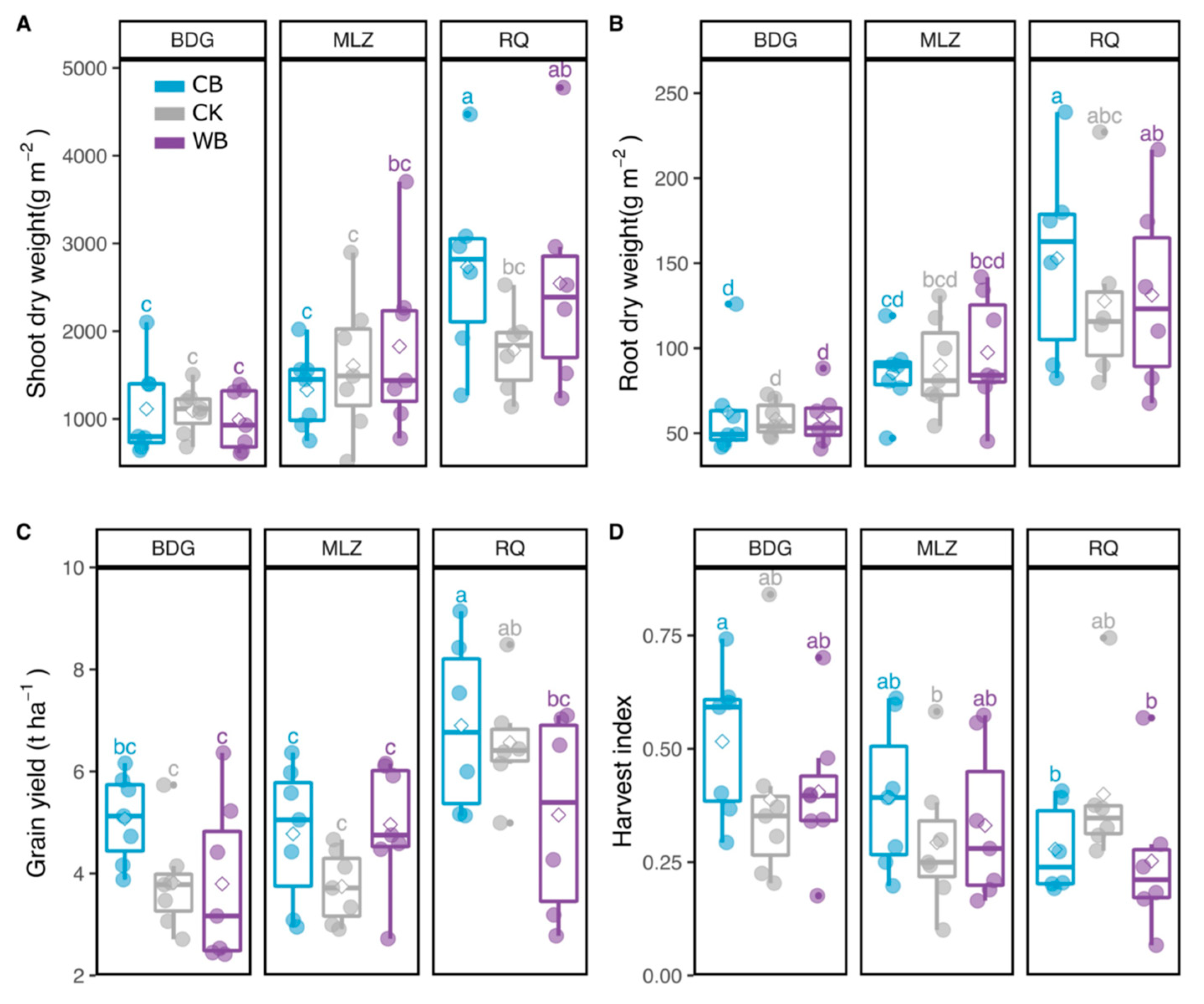
3.1. Biochar Effects on Plant Growth Indicators and Plant Nutrients Content

The CB and WB enhanced plant shoot dry weight by 48.7% and 45.0% in the field RQ in comparison to the CK, respectively (Figure 2A). Nevertheless, the enhancement was not found in the field BDG and MLZ. The field RQ indicated relatively a higher productivity than the field BDG and MLZ; there was no significant distinction of shoot dry weight between the three fields for the CK, while the shoot dry weight for the CB and WB treated soil in field RQ was significantly higher than in the BDG field. The root dry weight and grain yield were not significantly affected by biochar application, while they were significantly higher in the field RQ than BDG and MLZ for CK- and CB-treated soil (Figure 2B). Nevertheless, the mean value of the grain yield was increased by 29.7% and 35.1% by CB and WB application compared to the CK in the field MLZ (Figure 2C). The CB application also increased the mean value of the grain yield by 34.2% in the field BDG. The harvest index was not significantly affected by biochar in each field. However, the harvest index in the field BDG was significantly higher than in the field RQ for the CB-treated soil (Figure 2D).

The shoot TC, N, P, K, Mg, and root N and P concentration were not significantly enhanced by biochar in three fields (

Table 2. Plant nutrient concentrations under treatment of biochar in sandy clay loam (BDG and MLZ) and silty clay loam (RQ) soils.

Plant Nutrient Concentration (g kg−1)	BDG			MLZ			RQ
	CB	CK	WB	CB	CK	WB	CB	CK	WB
Shoot TC	467.09 ± 2.7 a	463.34 ± 3.58 a	466.8 ± 1.12 a	463.11 ± 2.88 a	463.23 ± 3.7 a	465.51 ± 1.7 a	468.59 ± 3.08 a	405.05 ± 67.55 a	406.56 ± 67.77 a
Shoot N	24.82 ± 0.64 a	23.29 ± 1.32 a	24.73 ± 1.24 a	24.84 ± 1.21 a	22.96 ± 0.78 a	25.54 ± 1.19 a	29.27 ± 1.69 a	29.17 ± 1.23 a	30.38 ± 1.61 a
Shoot P	3.7 ± 0.16 a	3.49 ± 0.18 a	3.7 ± 0.22 a	3.76 ± 0.21 a	3.66 ± 0.2 a	3.99 ± 0.26 a	3.55 ± 0.21 a	3.71 ± 0.17 a	3.94 ± 0.23 a
Shoot K	18.56 ± 0.44 a	16.96 ± 0.37 a	17.68 ± 0.69 a	16.6 ± 0.72 a	16.76 ± 1.14 a	17.28 ± 0.39 a	16.23 ± 0.56 a	17.4 ± 0.9 a	16.35 ± 0.91 a
Shoot Mg	5.48 ± 0.19 a	5.72 ± 0.3 a	5.42 ± 0.12 a	5.34 ± 0.14 a	5.14 ± 0.3 a	5.7 ± 0.2 a	5.1 ± 0.24 a	4.82 ± 0.15 a	4.56 ± 0.16 a
Root TC	467.49 ± 2.38 a	472.9 ± 4.02 a	468.26 ± 2.21 a	478.14 ± 2.65 a	463.87 ± 2.34 b	465.77 ± 1.8 b	477.71 ± 1.29 a	475.14 ± 1.54 a	480.19 ± 2.62 a
Root N	7.25 ± 0.17 a	8.17 ± 0.36 a	7.46 ± 0.33 a	7.12 ± 0.37 a	6.89 ± 0.3 a	7.08 ± 0.31 a	10.66 ± 0.56 a	10.08 ± 0.8 a	9.63 ± 0.63 a
Root P	1.37 ± 0.09 a	1.16 ± 0.08 a	1.14 ± 0.16 a	1.12 ± 0.15 a	1.19 ± 0.1 a	1.22 ± 0.13 a	1.3 ± 0.09 a	1.12 ± 0.15 a	1.09 ± 0.12 a
Root K	5.9 ± 0.24 a	5.25 ± 0.36 a	5.51 ± 0.36 a	5.51 ± 0.54 a	5.01 ± 0.54 a	4.91 ± 0.48 a	6.3 ± 0.3 a	5.98 ± 0.38 a	4.88 ± 0.39 b
Root Mg	1.82 ± 0.12 b	2.21 ± 0.06 a	1.8 ± 0.06 b	1.97 ± 0.15 a	2.34 ± 0.08 a	2.24 ± 0.14 a	2.25 ± 0.18 a	2.11 ± 0.22 a	1.79 ± 0.19 a

The means ± SE followed by a different letter within each column are significantly different at p < 0.05 using the Duncan-test.

). The CB application increased root C concentration by 3% in the field MLZ but not in the field BDG and RQ. The WB application indicated a lower root K concentration than the CK and CB in the field RQ. The CB and WB application significantly decreased the root Mg concentration by 17.6% and 18.6%, respectively, in the field BDG in comparison to the CK.

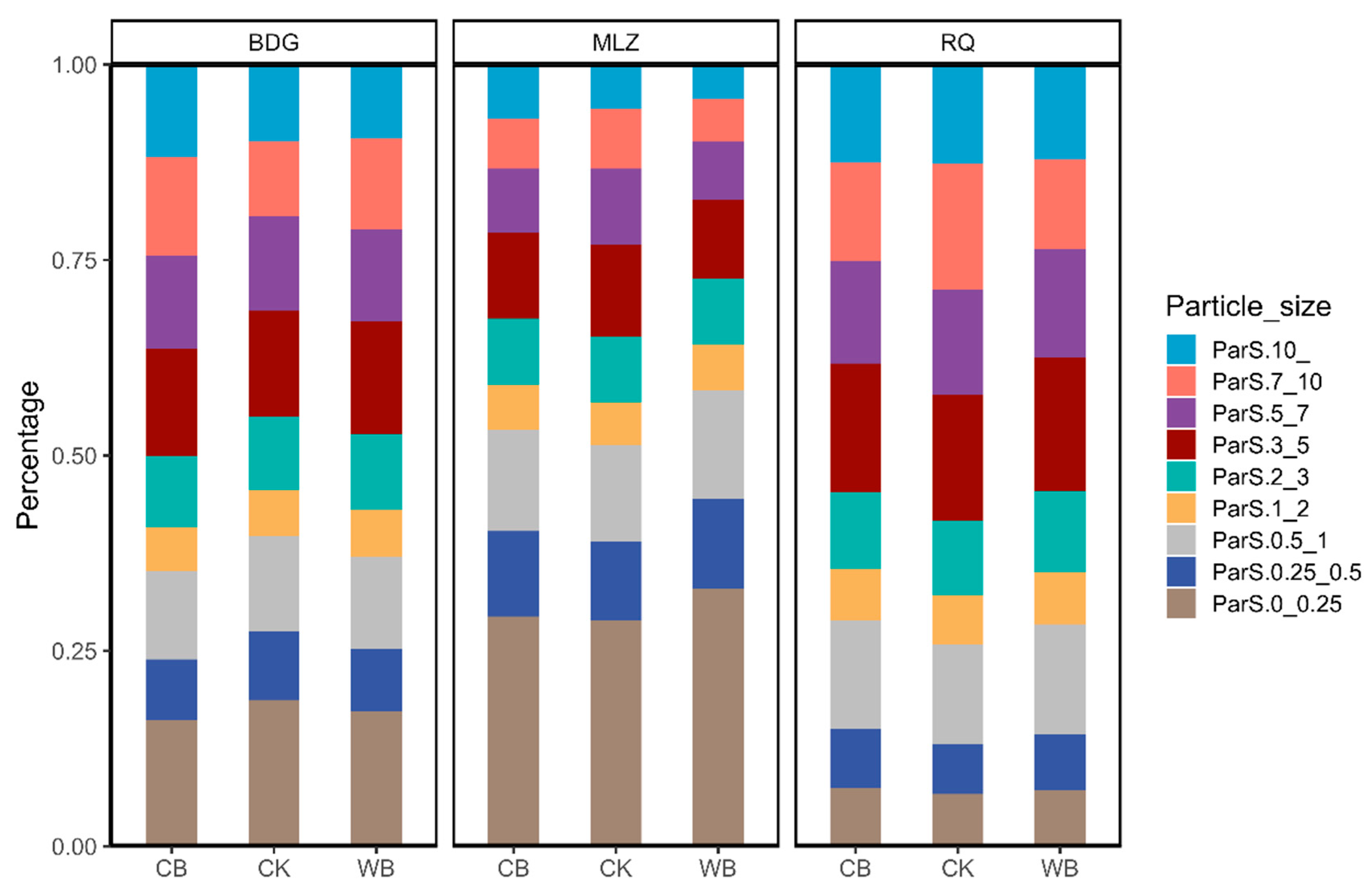
3.2. Biochar Effects on Lb Content and Soil Physicochemical Properties

The Lb content was not affected by biochar application, while it was significantly lower in the field RQ than BDG and MLZ for the CK- and WB-treated soil (Figure 3A). On the other hand, soil water content was much higher in the field RQ than BDG and MLZ for all three treatments (Figure 3B).

The MWD and GMD revealed no enhancement by biochar application, while they showed the lowest value in the field MLZ (Figure 3C,D). The GMD showed significantly higher in the field RQ than BDG for the CK, CB, and WB.

The CB application increased the proportion of 7–10 mm aggregates in the field BDG. The proportion of 0–0.25 mm, 0.25–0.5 mm, 0.5–1 mm, 1–2 mm, 2–3 mm, 3–5 mm, 5–7 mm, and >10 mm aggregates were not significantly affected by biochar in three fields (

Table 3. Soil aggregate size classes, nutrient concentrations, and porosity under treatment of biochar in sandy clay loam (BDG and MLZ) and silty clay loam (RQ) soils.

Soil Physicochemical Property	BDG			MLZ			RQ
	CB	CK	WB	CB	CK	WB	CB	CK	WB
>10 mm (%)	11.79 ± 1.63 a	9.76 ± 1.58 a	9.4 ± 1.67 a	6.94 ± 2.22 a	5.65 ± 1.01 a	4.4 ± 1.91 a	12.16 ± 1.64 a	12.18 ± 1.17 a	13.34 ± 1.31 a
7–10 mm (%)	12.66 ± 1.12 a	9.59 ± 1.01 b	11.63 ± 0.45 ab	6.28 ± 1.47 a	7.63 ± 0.97 a	5.37 ± 1.21 a	12.56 ± 1.58 a	15.12 ± 1.5 a	11.2 ± 0.89 a
5–7 mm (%)	11.85 ± 0.7 a	12.08 ± 0.88 a	11.79 ± 0.48 a	8.17 ± 0.98 a	9.77 ± 0.92 a	7.52 ± 1.21 a	12.96 ± 0.5 a	13.53 ± 0.68 a	13.39 ± 0.45 a
3–5 mm (%)	13.8 ± 0.47 a	13.54 ± 0.62 a	14.48 ± 0.9 a	10.93 ± 1.05 a	11.65 ± 0.82 a	10.03 ± 0.86 a	16.38 ± 0.39 a	15.96 ± 0.43 a	16.85 ± 0.46 a
2–3 mm (%)	9.02 ± 0.15 a	9.29 ± 0.5 a	9.66 ± 0.32 a	8.43 ± 0.5 a	8.43 ± 0.27 a	8.46 ± 0.37 a	9.91 ± 0.29 a	9.6 ± 0.35 a	10.12 ± 0.28 a
1–2 mm (%)	5.63 ± 0.08 a	5.91 ± 0.27 a	5.92 ± 0.19 a	5.69 ± 0.29 a	5.47 ± 0.23 a	5.82 ± 0.21 a	6.6 ± 0.36 a	6.33 ± 0.25 a	6.48 ± 0.24 a
0.5–1 mm (%)	11.29 ± 0.36 a	12.24 ± 0.58 a	11.82 ± 0.4 a	12.93 ± 0.62 a	12.4 ± 0.44 a	13.87 ± 0.57 a	13.82 ± 0.9 a	13.25 ± 0.75 a	13.44 ± 0.54 a
0.25–0.5 mm (%)	7.74 ± 0.36 a	8.69 ± 0.55 a	7.99 ± 0.37 a	10.88 ± 0.73 a	10 ± 0.42 a	11.47 ± 0.62 a	7.54 ± 0.67 a	6.78 ± 0.57 a	6.83 ± 0.38 a
0–0.25 mm (%)	16.17 ± 1.84 a	18.69 ± 1.27 a	17.23 ± 1.31 a	29.25 ± 2.98 a	28.89 ± 2.2 a	32.89 ± 3.46 a	7.85 ± 0.83 a	7.06 ± 0.64 a	7.11 ± 0.37 a
Soil TC (g kg−1)	26.46 ± 1.16 a	21.74 ± 0.58 b	22.68 ± 0.76 b	25.61 ± 0.93 a	23.59 ± 0.94 a	25.44 ± 1.16 a	36.31 ± 1.32 a	31.13 ± 0.77 b	33.6 ± 0.68 ab
Soil TN (g kg−1)	1.21 ± 0.03 a	1.12 ± 0.05 a	1.13 ± 0.05 a	1.03 ± 0.03 a	1 ± 0.02 a	1.07 ± 0.02 a	2.01 ± 0.08 a	1.87 ± 0.08 a	1.91 ± 0.03 a
Soil P (mg kg−1)	55.64 ± 2.84 a	56.3 ± 4.78 a	58.79 ± 4.86 a	46.17 ± 9.49 a	44.97 ± 5.42 a	49.76 ± 5.56 a	41.13 ± 4.87 a	36.37 ± 4.91 a	34.43 ± 1.6 a
Soil K (mg kg−1)	129.96 ± 24.53 a	134.48 ± 9.3 a	166.21 ± 13.81 a	124.49 ± 11.93 a	122.58 ± 7.85 a	114.09 ± 5.38 a	402.35 ± 49.77 a	287.2 ± 33.11 b	272.86 ± 12.08 b
Soil porosity (%)	42.19 ± 1.74 a	41.10 ± 1.20 a	40.64 ± 1.32 a	47.67 ± 1.56 a	46.59 ± 0.73 a	45.40 ± 1.25 a	45.07 ± 1.17 b	47.30 ± 1.12 ab	49.46 ± 1.22 a

The means ± SE followed by a different letter within each column are significantly different at p < 0.05 using the Duncan-test.

, Figure 4).

The CB application increased the soil TC concentration significantly in the field BDG and RQ (Table 3). The soil K concentration was also increased by the CB application in the field RQ. The soil N, P, and porosity were not significantly affected by biochar application.

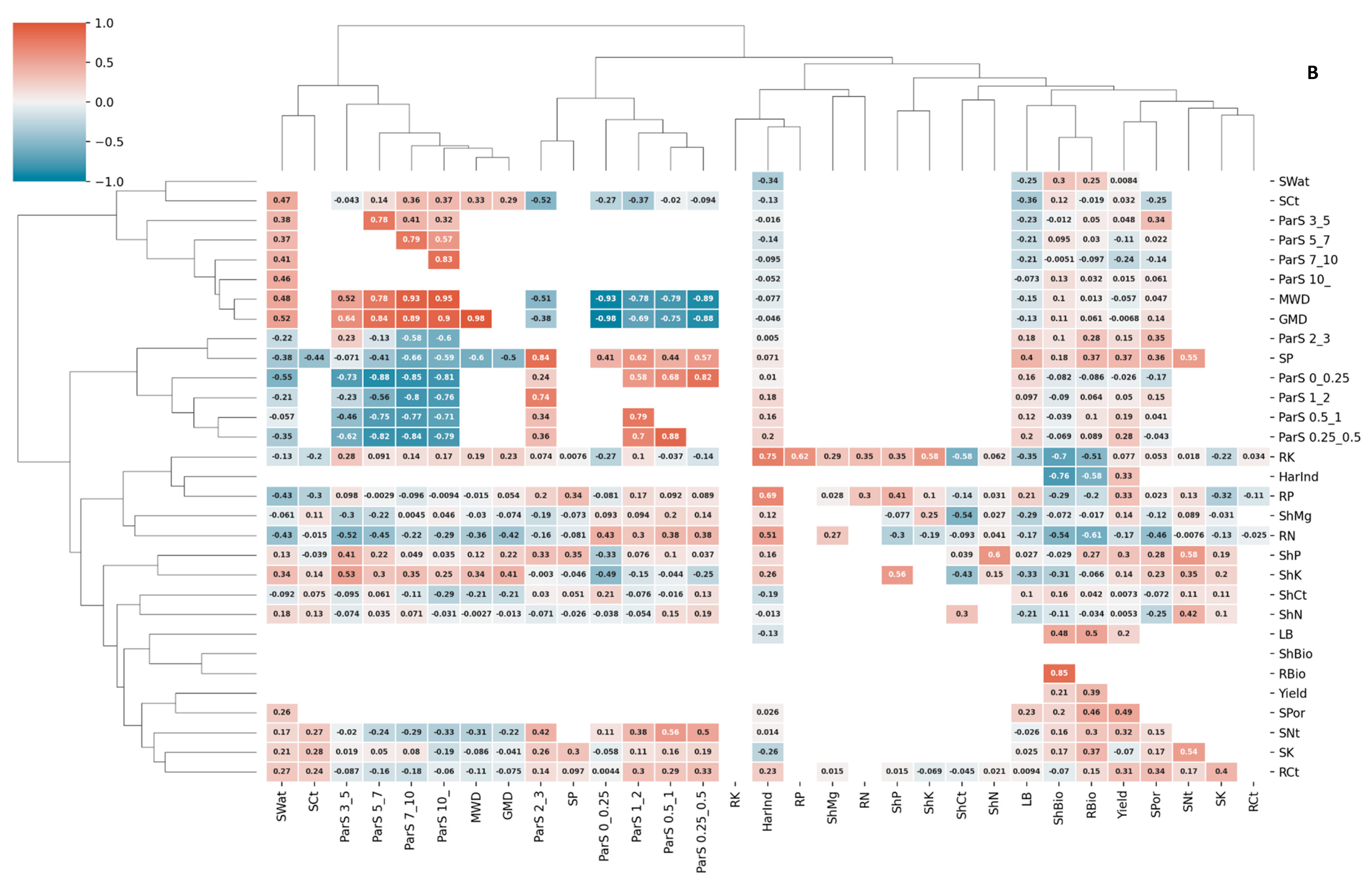
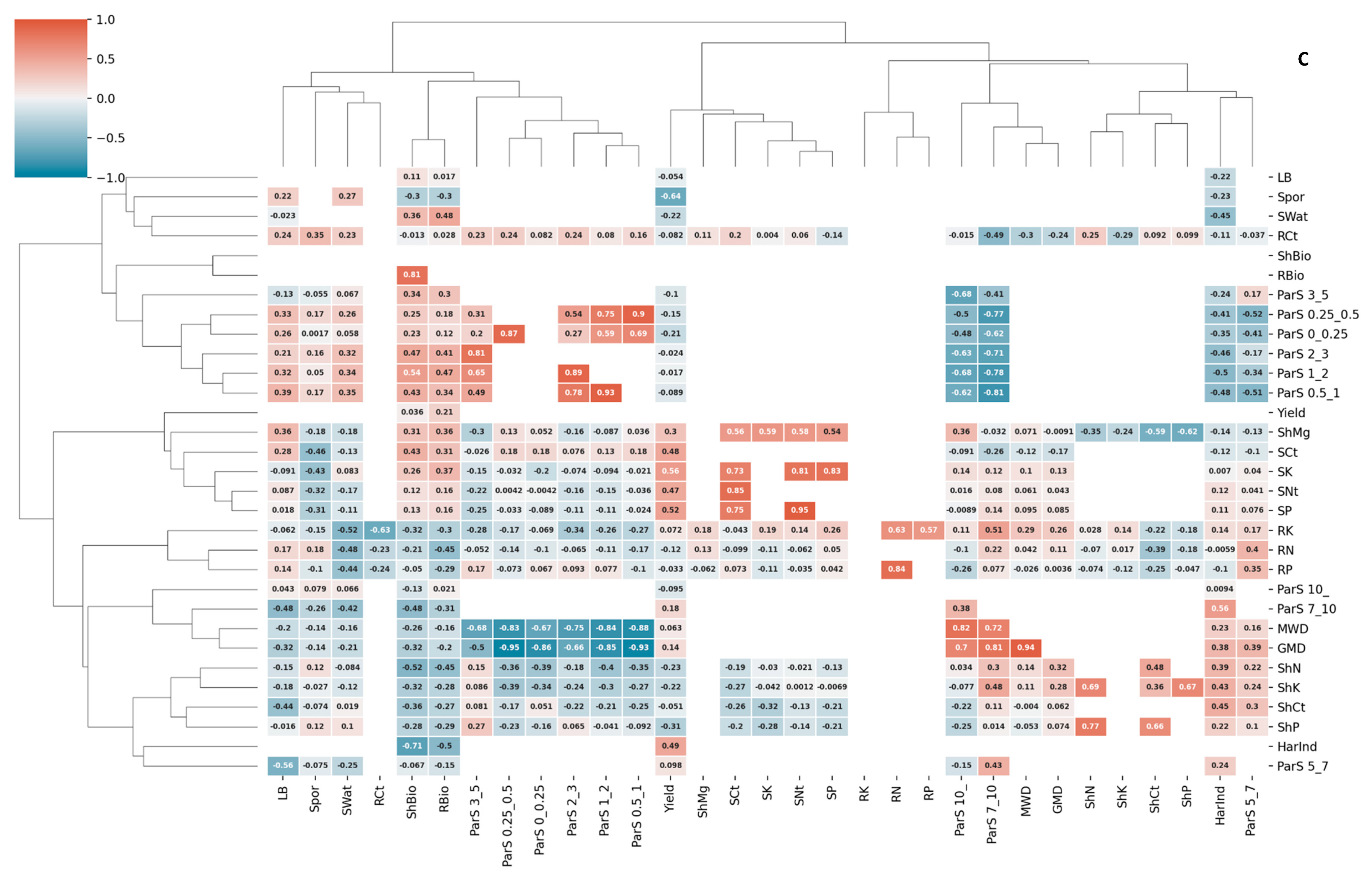
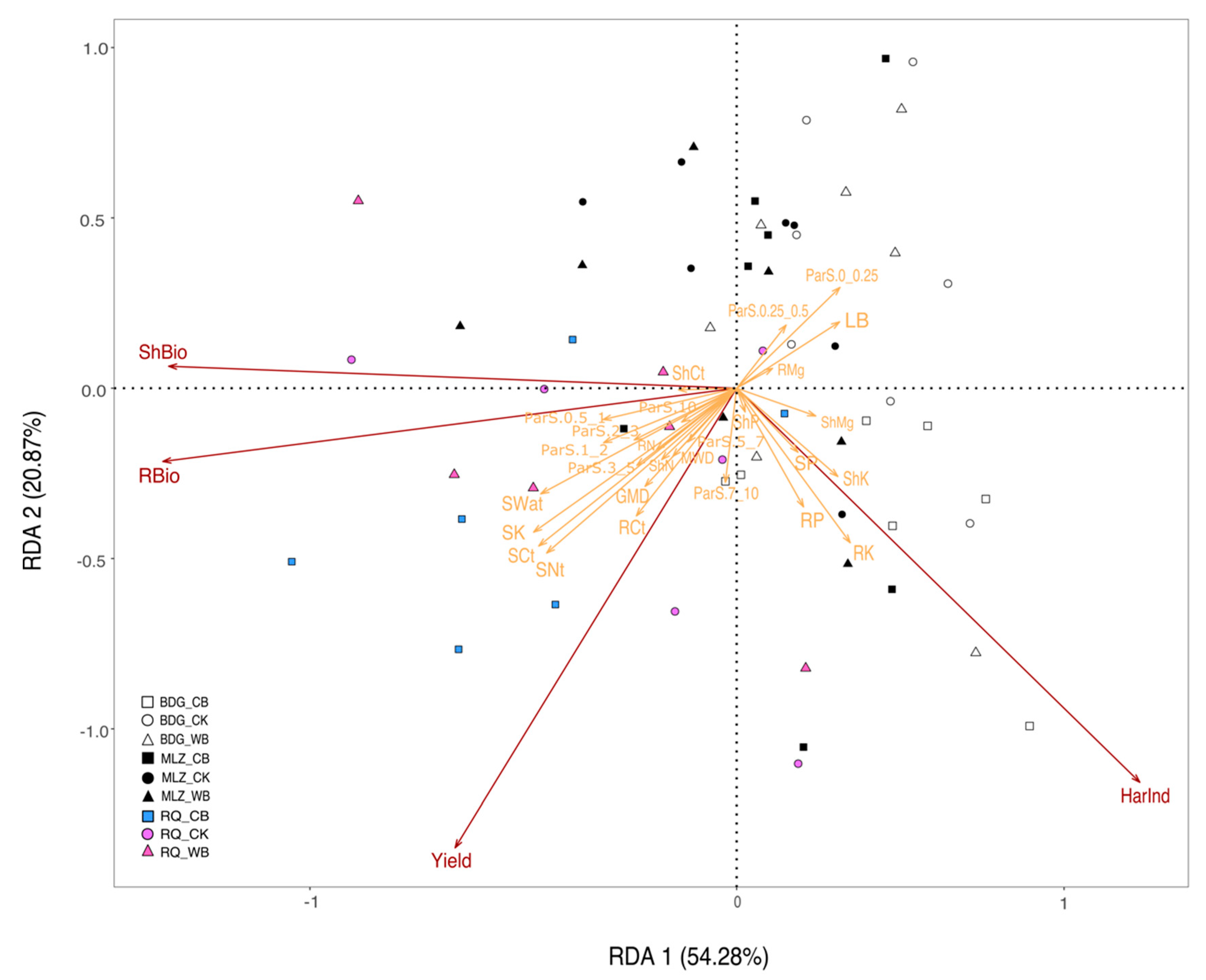
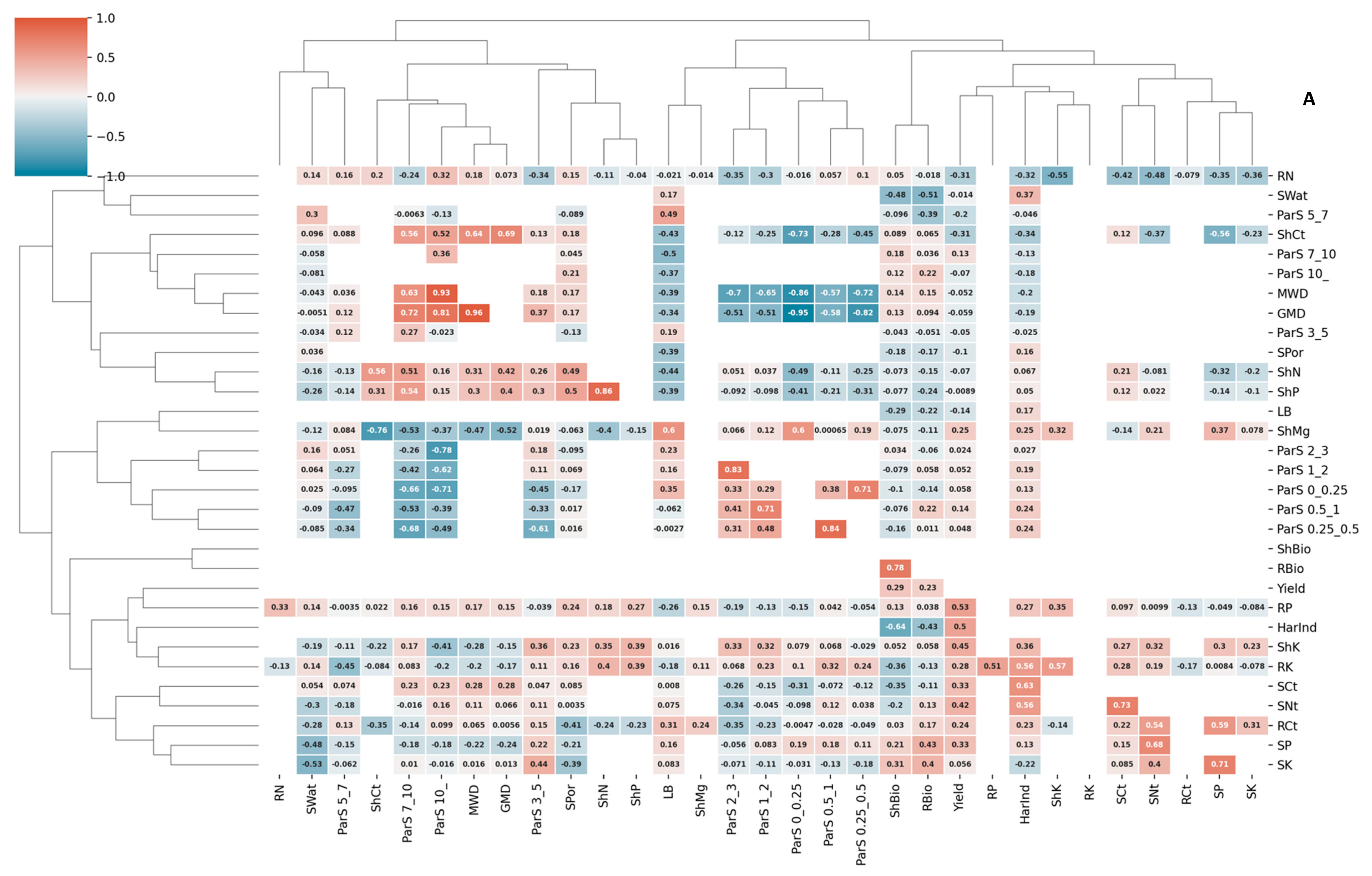
3.3. Correlations and Redundancy Analysis

For presenting the correlations between measurements, a cluster map was plotted separately for the data in three fields based on the Pearson correlation method (Figure 5). The hierarchical map indicates that all measurements can be classified into four clusters by correlations in each field. In all three fields, the soil water content was clustered separately, and the aggregate sizes 0–0.25 mm, 0.25–0.5 mm, 0.5–1 mm, 1–2 mm, and 2–3 mm were classified in the same cluster. The shoot biomass, root biomass, yield, harvest index, shoot K, root TC, root P, root K, soil TN, and soil K was classified in the same cluster in the field BDG and MLZ. The aggregate sizes 3–5 mm, 7–10 mm, >10 mm, MWD, and GMD were also classified in the same cluster in the field BDG and MLZ. Dissimilarly, the shoot biomass, root biomass, and aggregate size 3–5 mm were classified together with the aggregate sizes 0–0.25 mm, 0.25–0.5 mm, 0.5–1 mm, 1–2 mm, and 2–3 mm in RQ field. The aggregate sizes 5–7 mm, 7–10 mm, >10 mm, MWD, and GMD were classified in the same cluster with the harvest index, shoot TC, shoot N, shoot P, shoot K, root N, root P, and root K.

Specifically, the shoot biomass and root biomass showed a strong correlation with aggregate sizes 0.5–1 mm, 1–2 mm, and 2–3 mm and soil water content in the field RQ. However, these correlations were not observed in the other two fields. The yield and harvest index showed no correlation with any aggregate size in the three fields. The Lb content showed a stronger correlation with the aggregate sizes of 0–0.25 mm, 0.25–0.5 mm, 0.5–1 mm, 1–2 mm, and 2–3 mm in the RQ field than in the other two fields. The Lb content indicated the negative correlations with the aggregate size of 7–10 mm in all three fields. The soil K showed a strong correlation with shoot biomass and root biomass in three fields.

The RDA was conducted using the standardized data of response variables (red vectors in Figure 6) and explanatory variables (orange vector in Figure 6). The first and second RDA axes explained 54.28% and 20.87% of the total variance with the significance level at p < 0.001 and p < 0.05, respectively (Figure 6,

Table 4. Permutation test for RDA under reduced model.

		Df	Variance	F	Pr (>F)	Signif.
Model		28	3.14359	4.064	0.001	***
Axis	RDA1	1	2.17135	139.448	0.001	***
	RDA2	1	0.83498	53.624	0.042	*
	RDA3	1	0.09565	6.143	1
	RDA4	1	0.04161	2.672	1
Explanatory variables	LB	1	0.25295	7.7685	0.002	**
	SWat	1	0.61597	18.9176	0.001	***
	SPor	1	0.0523	1.6061	0.221
	ParS.10_	1	0.026	0.7985	0.451
	ParS.7_10	1	0.18183	5.5843	0.005	**
	ParS.5_7	1	0.03474	1.0669	0.321
	ParS.3_5	1	0.00306	0.0941	0.953
	ParS.2_3	1	0.00229	0.0703	0.966
	ParS.1_2	1	0.01708	0.5246	0.596
	ParS.0.5_1	1	0.03285	1.009	0.374
	ParS.0.25_0.5	1	0.04492	1.3795	0.254
	ParS.0_0.25	1	0.21643	6.6471	0.007	**
	MWD	1	0.13205	4.0555	0.03	*
	GMD	1	0.05726	1.7586	0.174
	SCt	1	0.19856	6.098	0.005	**
	SNt	1	0.0222	0.6818	0.498
	SP	1	0.04169	1.2803	0.26
	SK	1	0.15023	4.6137	0.02	*
	ShCt	1	0.06954	2.1358	0.096
	ShN	1	0.04044	1.2421	0.279
	ShP	1	0.0867	2.6627	0.075
	ShK	1	0.10648	3.2703	0.046	*
	ShMg	1	0.03127	0.9604	0.405
	RCt	1	0.03391	1.0413	0.379
	RN	1	0.06323	1.9418	0.143
	RP	1	0.20455	6.2822	0.004	**
	RK	1	0.26496	8.1373	0.002	**
	RMg	1	0.00711	0.2184	0.83
Residual		31	1.00939

Df, degree of freedom; Variance, the variance of accumulated constrained eigenvalues; F, F-value; Pr(>F), p-value; Signif., significance level; Signif. codes: ***: p < 0.001, **: p < 0.01, *: p < 0.05.

). Transformed observations in triplot indicated separations between the field BDG and RQ, MLZ, and RQ, respectively. For the field BDG, the triplot showed a separation between CK and CB (Figure 6).

The importance of the model, axes, and the explanatory variables were tested for RDA (Table 4). The significance level of the RDA model reveals that the data can be explained by the model properly. The RDA1 axis explained the most of variables and showed significant importance (Table 4). The Lb, soil water content, aggregate 7–10 mm, aggregate 0–0.25 mm, MWD, soil TC, soil K, shoot K, root P, and root K indicated significant importance in explaining plant growth indicators.

3.4. Ridge Regression

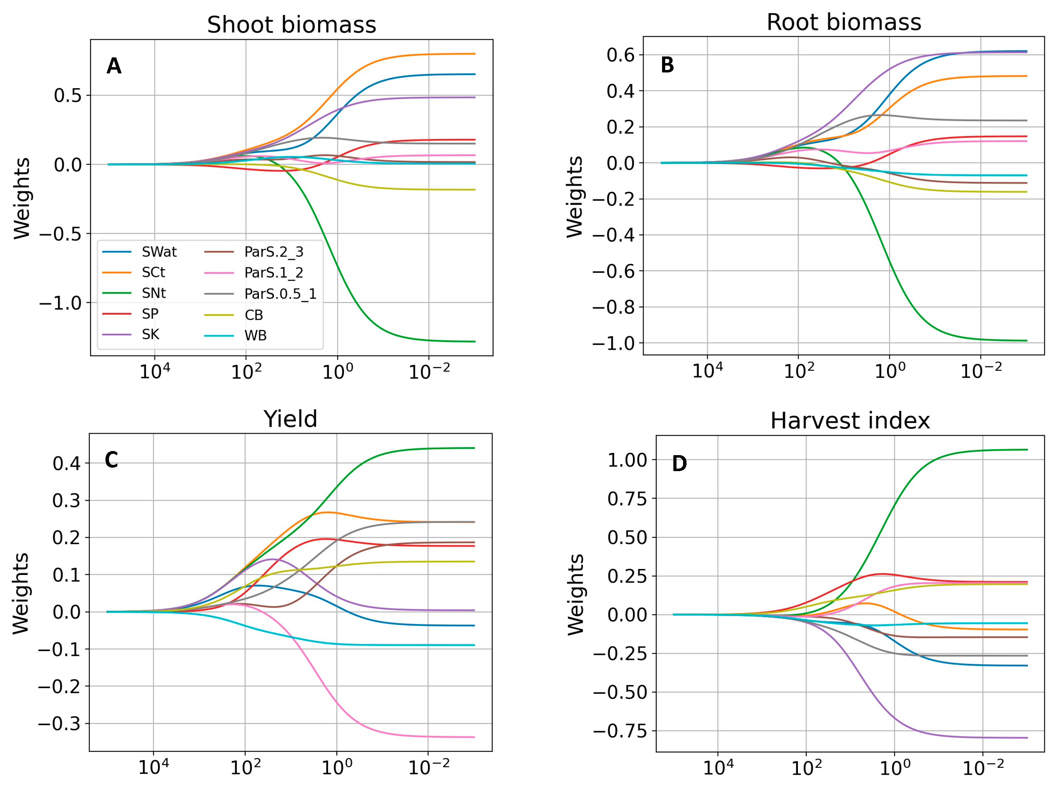
3.4.1. Determination of Regularization Parameter

The trace plot of ridge regression was visualized to show the values of the regression coefficient responding to α (Figure 7). In the trace plot, where the most coefficient estimates tend to be zero, the value of α is considered to be optimal for the regression. In the trace plot of shoot biomass, root biomass, yield, and harvest index (Figure 7), most of the coefficient estimates start to shrink towards zero at α = 10. Additionally, we used cross-validation to verify the values of α. The values 0.1, 1, and 10 for α are compared for cross-validation based on the performance of the model. Then, a value of α was selected considering the smallest loss of cross-validation. Those optimal values of α selected in the trace plot were validated here, and these values of α were used for regression model establishment.

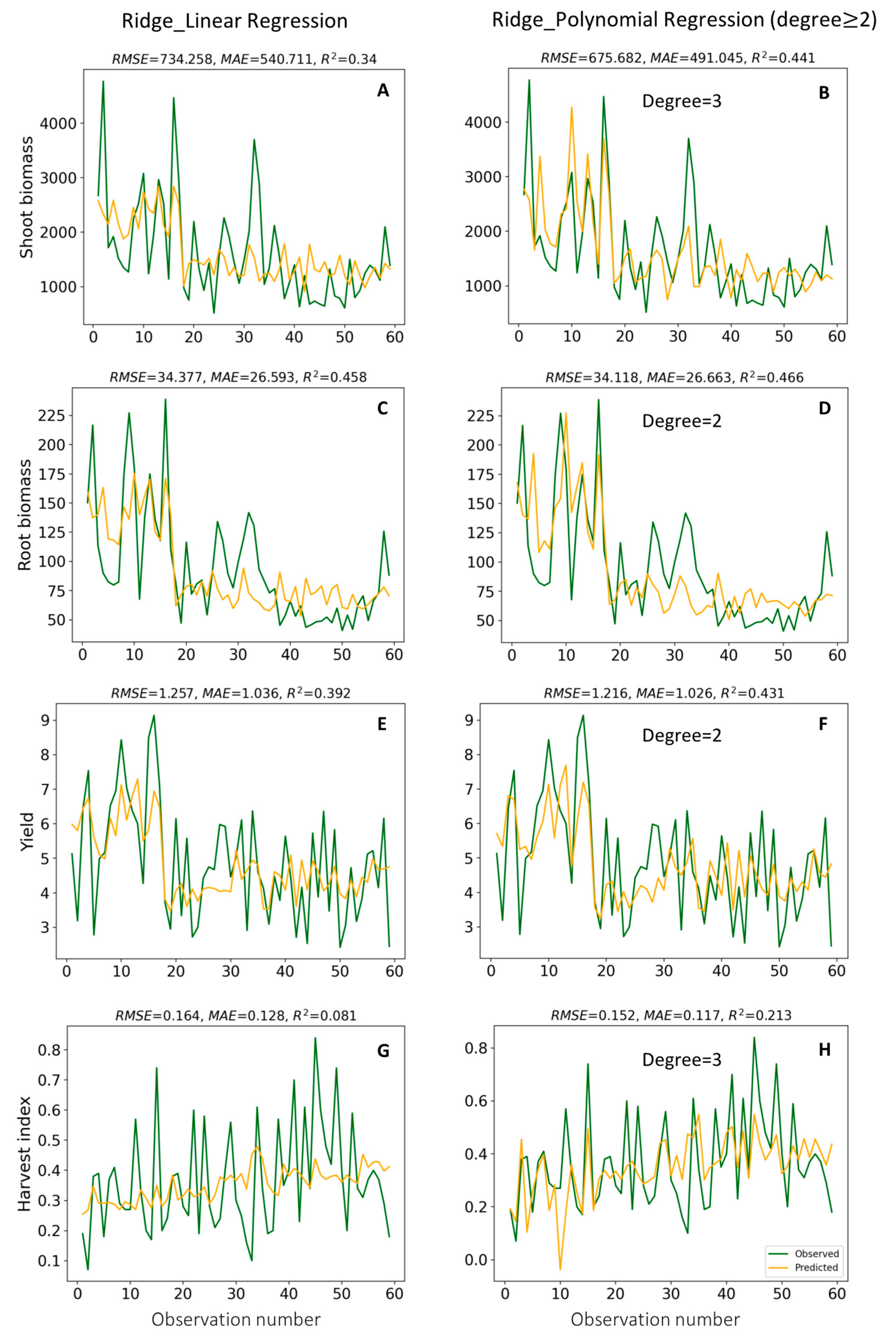
3.4.2. Prediction of Soybean Growth Indicators

We examined a range of exponential degrees for the polynomial model to determine an optimal regression method. We observed that a higher degree accompanies a better training score, but the testing score will reach a peak at a degree and then present a decline subsequently with the degree increasing. In this case, the regression is easier to be overfitted. On contrary, linear polynomial regression is liable to be underfitted (Figure 8). Therefore, an optimal exponential degree should be considered by a balance of the determinant coefficient of the train-set and test-set data. By conducting a range of tests, we confirmed the quadratic polynomial regression is optimal for root biomass and yield prediction, while the cubic polynomial regression is optimal for shoot biomass and harvest index prediction (Figure 8).

Overall, the prediction accuracy of the exponential polynomial model is better than the linear regression model (Figure 8). Predictions of shoot biomass and harvest index revealed a much better correspondence with observed values, while the exponential polynomial model was employed in comparison to the linear regression model (Figure 8A,B,G,H). The correspondence of predicted root biomass and yield with observed values was not much improved by employing the exponential polynomial model in comparison to the linear regression model (Figure 8C–F).

4. Discussion

4.1. Plant Growth

The biochar has been observed to increase the yield or plant biomass of leguminous crops [38,39,40,41,42,43]. It was also reported that the grain yield of soybean and common bean was increased ranging from 23% to 54% by biochar [38,44]. Biochar showed the potential to enhance plant growth and grain yield formation. On the other hand, it was also reported that 10 t ha⁻¹ of biochar application showed no increase in soybean yield [45], and some research even indicated inhibition of plant growth by biochar application [44,46,47,48]. It shows the intricacy of the effect of biochar on plant growth. In this study, the cob biochar increased the shoot biomass but not the grain yield in the silty clay loam soil, thus resulting in a low harvest index. By all appearances, the shoot growth and seed development were imbalanced for soybean production. It might be caused by the vegetative growth of soybean competing for water and nutrients with reproductive growth [49]. It has also been reported that the meristems allocation is influenced by shoot competition [49]. The shoot competition was also reflected in the correlations between the biomass or grain yield and soil water content in silty clay loam soil. The correlation between the soil water content and shoot biomass or root biomass was positive in the silty clay loam soil, while the grain yield showed a negative correlation with the soil water content. Water supply promoted the biomass increase but resulted in excessive vegetative growth, and thus, the reproductive growth was restricted. Generally, the increase of plant height costs lateral growth when it is in adequate water conditions [50,51,52]. On the other hand, in sandy clay loam soils, the biomass was limited by the low soil water content; in turn, the meristems allocation to the grain yield was balanced. Especially, in the field BDG, the harvest index was relatively higher than in the other two fields. In addition, the RDA results also supports the above demonstration since the data distribution of the field BDG tends to be closer to the harvest index than the other two fields in the RDA plot. It reflects that the field BDG explains more harvest index. Especially, the data cluster of cob biochar in the field BDG showed the closest relationship with the harvest index. By contrast, the data distribution of the silty clay loam soil is close to shoot and root biomass. The performance of the yield in cob-biochar-treated plots in sandy clay loam soils was better than in control plots even if there was no significant difference in statistics. It still shows the potential of cob biochar application to enhance soil productivity in desertified areas.

4.2. Soil Aggregation

The use of biochar showed no significant effect on most soil aggregate sizes in this study. In parallel, it was also reported that biochar was ineffective in soil aggregation [23]. Soil aggregate stability could be enhanced by organic matter. Especially, the humic substances, which are usually derived from organic matter decomposition, could serve as a soil conditioner to enhance aggregate stability [53]. Although biochar is organic matter, it could not be readily decomposed in the soil, so it is not an ideal organic source of humic substances.

Soil aggregation has been reported to be based on soil type, and therefore, the soil structure is highly related to soil type [11]. Ciric et al. (2012) found soil type has a significant effect on all aggregate size classes (ASCs) and structure indices [11]. In this study, the ASCs distribution also varied in the silty clay loam soil and sandy clay loam soils. In all ASCs, aggregate sizes 0.5–1 mm, 1–2 mm, and 2–3 mm play important roles in plant biomass formation in the silty clay loam soil due to the positive correlation between these aggregate sizes with the shoot and root biomass in the silty clay loam soil. We noticed that these aggregate sizes also showed a positive correlation with the soil water content. A high proportion of agronomically valuable aggregates usually corresponds to soils with optimal water-holding capacity [13]. Therefore, the variation of the water content with these aggregate sizes may affect soybean biomass.

The silty clay loam soil showed the highest value of mean weight diameter (MWD) and geometric mean diameter (GMD), which differed from the sandy clay loam soils. Higher MWD represents higher water permeability, air capacity, and aggregate stability in soil [11,13]. The low MWD of sandy clay loam soils showed a negative effect of desertification on the soil structure and soil water content in the study area. The GMD is regarded as a predictor of wind erosion [14]. The low GMD of sandy clay loam soils indicated that the desertification made the field more vulnerable to wind erosion and reduced the soil aggregate stability. Causally, wind erosion removes more unstable aggregates from the soil surface [14,54]. The removal of microaggregates, which contain large amounts of nutrients and organic carbon, leads to a decrease in soil fertility [14,55]. Gradually, the soil sinks into such a dead circulation, and the soil quality turns lower and lower. To maintain soil productivity, protection of the land by field management should be considered. Such managements include crop residues management, proper fertilizer, and irrigation application, incorporation, and biological N-fixation introduction [56].

4.3. Nitrogen Fixation Ability

Chemical N fertilizer is a major source of N input in cropping systems. It may lead to a cost of energy and labor during fertilizer product transporting and application. In addition, the N leaching and fertilizer transportation will result in environmental damage [57,58]. Biological N fixation is a sustainable N source in the soybean cropping system, and it can produce as much as 450 kg ha⁻¹ of N by nodules [5]. The Lb takes 40% of all nodule protein and plays important role in N fixation [6]. The Lb responded to the aggregate sizes 0–0.25 mm, 0.25–0.5 mm, 0.5–1 mm, 1–2 mm, and 2–3 mm but not to 7–10 mm, according to their correlations. The better ventilation between aggregate sizes 0–0.25 mm, 0.25–0.5 mm, 0.5–1 mm, 1–2 mm, and 2–3 mm provides more O₂ for Lb, and thus, the Lb may support the energy metabolism through its O2-binding heme group in nodules for the demand of the symbiont N fixation [6]. The low water content of sandy clay loam soil resulted in a high soil air content. Consequently, the sandy clay loam soil indicated a higher Lb content than silty clay loam soil, and thus, the high N-fixation ability of the soybean cropping system in desertified land may provide a sustainable N source to relieve the overusing of N fertilizer. It is of vital consequence to the protection of vulnerable ecosystems in the desertified area.

4.4. Modelling of Plant Growth Indicators

To sustain the soil productivity and conserve the agri-ecosystem, the modeling for precise control of field management is crucial. The modeling of plant growth indicators may provide a reference quantity for fertilization, irrigation, and soil amendment application according to the accurate requirement of plant growth. The model of OLS regression ignores the problems of multicollinearity, which renders parameter estimates’ fluctuation. Ridge regression may solve the problems of multicollinearity [33,37] and improve the accuracy of prediction [31,32]. The addition of shrinkage penalty, will improve the model performance of exponential polynomial regression or linear regression in the machine learning techniques. The modeling is liable to be overfitted while we conduct exponential polynomial regression. Proper exponential degree determination will facilitate solving problems of overfitting [59]. We obtained the optimal exponential degrees for plant growth indicator prediction by balancing the performance of the train-set and test-set in the model.

The cubic polynomial regression ameliorated the accuracy of prediction of the shoot biomass and harvest index largely in comparison to the linear regression since the predicted values showed good correspondence to observed values. Although the quadratic polynomial regression performed better than the linear regression to predict the root biomass and grain yield, the difference was not large. Overall, the predicted values of the shoot biomass, root biomass, and grain yield showed a good correspondence with observed values as well as a good R². Even so, the bias between the predicted and observed values remained. The predictors of soil nutrients, soil aggregate sizes, and biochar can predict the shoot biomass, root biomass, and grain yield, but the prediction accuracy still needs to be improved. On the other hand, it is hard to estimate harvest index by soil nutrients, soil aggregate sizes, and biochar due to the weak performance of the model with quite low R². As discussed above, the harvest index patterns are varied in different types of soil. The meristems allocation to the grain yield was balanced in the sandy clay loam soils but imbalanced in the silty clay loam soil. Therefore, balancing the vegetative and reproductive growth of plants by field management is crucial to improving soybean production.

5. Conclusions

Desertified land occupies a large area of the world. Two major measures together for combating desertification are controlling its expansion and managing to utilize desertified land for agricultural production. The measures facilitate meeting the high demand for food in the desertification-affected area. This case study provided fundamental information to demonstrate the potential for utilizing the desertified land. Even if the overall soil productivity in sandy clay loam soil is lower than in silty clay loam soil, the harvest index indicated similarities between the two kinds of soils, or the average harvest index of sandy clay loam soil even tends to be higher. It demonstrates that the sandy clay loam soil may also have high efficacy for crop production while the balance between vegetative and reproductive growth is well manipulated.

Soil type dominated the influence on plant growth and soil aggregation rather than biochar. Aggregate sizes 0.5–1 mm, 1–2 mm, and 2–3 mm indicated more importance in plant biomass formation in silty clay loam soil. The soil aggregate sizes 0–0.25 mm, 0.25–0.5 mm, 0.5–1 mm, 1–2 mm, and 2–3 mm are ideal for Lb formation, but the size of 7–10 mm is negatively related to the Lb formation. The low aggregate stability of sandy clay loam soil drove the field more vulnerable to wind erosion in the semi-arid monsoon climate. The biochar produced by maize cob may increase shoot biomass in silty clay loam soil but not in sandy clay loam soil. However, biochar application showed limiting effect on root biomass, grain yield, and harvest index.

The higher N-fixing ability of nodules in sandy clay loam soil indicates an advantage to reduce the use of N-fertilizers in desertified areas. The N fixation thus reduces cropping cost and alleviates the pressure of fertilizer overusing on ecosystem health. Therefore, legume cultivation can be a strategic measure for establishing a sustainable cropping system in desertified areas.

Exponential polynomial regression ameliorated the accuracy of prediction of plant growth indicators in comparison to linear regression. Shoot biomass, root biomass, and grain yield can be predicted by soil nutrients, soil aggregate sizes, and biochar, but the prediction accuracy still needs to be improved in further study.

References

1. Longjun, C. UN convention to combat desertification. In Encyclopedia of Environmental Health; Elsevier: Amsterdam, The Netherlands, 2019; pp. 238–251. [Google Scholar]
2. UNCCD. United Nations Convention to Combat Desertification. 2022. Available online: https://www.unccd.int/our-work/land-life-programme (accessed on 30 May 2022).
3. Qin, L.; Jiang, H.; Tian, J.; Zhao, J.; Liao, H. Rhizobia: Enhance acquisition of phosphorus from different sources by soybean plants. Plant Soil 2011, 349, 25–36. [Google Scholar] [CrossRef]
4. Dos Santos Silva, F.C.; Sediyama, T.; de Cássia Teixeira Oliveira, R.; Borém, A.; da Silva, F.L.; Bezerra, A.R.G.; da Silva, A.F. Economic Importance and Evolution of Breeding. In Soybean Breeding; Da Silva, F.L., Gomes Bezerra, A.R., da Silva, A.F., Eds.; Springer: Cham, Switzerland, 2017; p. 3. [Google Scholar]
5. Salvagiotti, F.; Cassman, K.G.; Weiss, A.; Dobermann, A. Nitrogen Uptake, Fixation and Response to N Fertilizer in Soybeans. Field Crops Res. 2008, 108, 1–13. [Google Scholar] [CrossRef] [Green Version]
6. Jiang, S.; Jardinaud, M.F.; Gao, J.; Pecrix, Y.; Wen, J.; Mysore, K.; Xu, P.; Sanchez-Canizares, C.; Ruan, Y.; Li, Q.; et al. NIN-like protein transcription factors regulate leghemoglobin genes in legume nodules. Science 2021, 374, 625–628. [Google Scholar] [CrossRef]
7. Pirmoradian, N.; Sepaskhah, A.R.; Hajabbasi, M.A. Application of fractal theory to quantify soil aggregate stability as influence by tillage treatments. Biosyst. Eng. 2005, 90, 227–234. [Google Scholar] [CrossRef]
8. Wei, C.; Gao, M.; Shao, J.; Xie, D.; Pan, G. Soil aggregate and its response to land management practices. China Particuology 2006, 4, 211–219. [Google Scholar] [CrossRef]
9. Barthès, B.; Roose, E. Aggregate stability as an indicator of soil susceptibility to runoff and erosion; validation at several levels. Catena 2022, 47, 133–149. [Google Scholar] [CrossRef] [Green Version]
10. Cantón, Y.; Solé-Benet, A.; Asensio, C.; Chamizo, S.; Puigdefábregas, J. Aggregate stability in range sandy loam soils relationships with runoff and erosion. Catena 2009, 77, 192–199. [Google Scholar] [CrossRef] [Green Version]
11. Ciric, V.; Manojlovic, M.; Nesic, L.; Belic, M. Soil dry aggregate size distribution: Effects of soil type and land use. J. Soil Sci. Plant Nutr. 2012, 12, 689–703. [Google Scholar] [CrossRef] [Green Version]
12. Bünemann, E.K.; Bongiorno, G.; Bai, Z.; Creamer, R.E.; De Deyn, G.; de Goede, R.; Fleskens, L.; Geissen, V.; Kuyper, T.W.; Mader, P.; et al. Soil Quality—A Critical Review. Soil Biol. Biochem. 2018, 120, 105–125. [Google Scholar] [CrossRef]
13. Smirnova, L.G.; Novykh, L.L.; Pelekhotse, E.A. Physical properties of chernozems on slopes in the landscape farming system. Eurasian Soil Sci. 2006, 39, 278–282. [Google Scholar] [CrossRef]
14. Shahabinejad, N.; Mahmoodabadi, M.; Jalalian, A.; Chavoshi, E. The fractionation of soil aggregates associated with primary particles influencing wind erosion rates in arid to semiarid environments. Geoderma 2019, 356, 113936. [Google Scholar] [CrossRef]
15. McKenzie, B.M.; Tisdall, J.M.; Vance, W.H. Soil Physical Quality. In Encyclopedia of Agrophysics; Encyclopedia of Earth Sciences Series; Gliński, J., Horabik, J., Lipiec, J., Eds.; Springer: Dordrecht, The Netherlands, 2011; pp. 770–777. [Google Scholar]
16. Magdoff, F. Soil Quality and Management. In Agroecology; CRC Press: Boca Raton, FL, USA, 2018; pp. 349–364. [Google Scholar]
17. Atkinson, C.J.; Fitzgerald, J.D.; Hipps, N.A. Potential mechanisms for achieving agricultural benefits from biochar application to temperate soils: A review. Plant Soil 2010, 337, 1–18. [Google Scholar] [CrossRef]
18. Biederman, L.A.; Harpole, W.S. Biochar and its effects on plant productivity and nutrient cycling: A meta-analysis. GCB Bioenergy 2013, 5, 202–214. [Google Scholar] [CrossRef]
19. Brodowski, S.; John, B.; Flessa, H.; Amelung, W. Aggregate occluded black carbon in soil. Eur. J. Soil Sci. 2006, 57, 539–546. [Google Scholar] [CrossRef]
20. Liang, B.; Lehmann, J.; Solomon, D.; Sohi, S.; Thies, J.E.; Skjemstad, J.O.; Luizão, F.J.; Engelhard, M.H.; Neves, E.G.; Wirick, S. Stability of biomass-derived black carbon in soils. Geochim. Cosmochim. Acta 2008, 72, 6069–6078. [Google Scholar] [CrossRef]
21. Purakayastha, T.J.; Kumari, S.; Sasmal, S.; Pathak, H. Biochar carbon sequestration in soil-A myth or reality? Int. J. Bio Resour. Stress Manag. 2015, 6, 623–630. [Google Scholar] [CrossRef]
22. Kumari, K.G.I.D.; Moldrup, P.; Paradelo, M.; Elsgaard, L.; de Jonge, L.W. Soil Properties Control Glyphosate Sorption in Soils Amended with Birch Wood Biochar. Water Air Soil Pollut. 2016, 227, 174. [Google Scholar] [CrossRef]
23. Busscher, W.J.; Novak, J.M.; Evans, D.E.; Watts, D.W.; Niandou, M.A.S.; Ahmedna, M. Influence of pecan biochar on physical properties of a Norfolk loamy sand. Soil Sci. 2010, 175, 10–14. [Google Scholar] [CrossRef] [Green Version]
24. Peng, X.; Ye, L.L.; Wang, C.H.; Zhou, H.; Sun, B. Temperature- and duration-dependent rice straw-derived biochar: Characteristics and its effects on soil properties of an Ultisol in southern China. Soil Tillage Res. 2011, 112, 159–166. [Google Scholar] [CrossRef]
25. Hardie, M.; Clothier, B.; Bound, S.; Oliver, G.; Close, D. Does biochar influence soil physical properties and soil water availability? Plant Soil 2014, 376, 347–361. [Google Scholar] [CrossRef]
26. Sohi, S.; Lopez-Capel, E.; Krull, E.; Bol, R. Biochar, climate change and soil: A review to guide future research. Capel 2009, 5, 17–31. [Google Scholar]
27. Ma, H.; Shurigin, V.; Jabborova, D.; Dela Cruz, J.A.; Dela Cruz, T.E.; Wirth, S.; Bellingrath-Kimura, S.D.; Egamberdieva, D. The Integrated Effect of Microbial Inoculants and Biochar Types on Soil Biological Properties, and Plant Growth of Lettuce (Lactuca sativa L.). Plants 2022, 11, 423. [Google Scholar] [CrossRef] [PubMed]
28. Egamberdieva, D.; Li, L.; Ma, H.; Wirth, S.; Bellingrath-Kimura, S.D. Soil amendments with different maize biochars, to varying degrees, improve chickpea growth under drought by improving symbiotic performance with Mesorhizobium ciceri and soil bio-chemical properties. Front. Microbiol. 2019, 10, 2423. [Google Scholar] [CrossRef]
29. Egamberdieva, D.; Shurigin, V.; Alaylar, B.; Ma, H.; Müller, M.E.H.; Wirth, S.; Reckling, M.; Bellingrath-Kimura, S.D. The effect of biochars and endophytic bacteria on growth and root rot disease incidence of Fusarium infested narrow-leafed lupin (Lupinus angustifolius L.). Microorganisms 2020, 8, 496. [Google Scholar] [CrossRef] [PubMed] [Green Version]
30. Salazar, J.J.; Garland, L.; Ochoa, J.; Pyrcz, M.J. Fair train-test split in machine learning: Mitigating spatial autocorrelation for improved prediction accuracy. J. Pet. Sci. Eng. 2022, 209, 109885. [Google Scholar] [CrossRef]
31. Bedoui, A.; Lazar, N.A. Bayesian empirical likelihood for ridge and lasso regressions. Comput. Stat. Data Anal. 2020, 145, 106917. [Google Scholar] [CrossRef]
32. Panzone, L.; Ulph, A.; Areal, F.; Grippo, V. A ridge regression approach to estimate the relationship between landfill taxation and waste collection and disposal in England. Waste Manag. 2021, 129, 95–110. [Google Scholar] [CrossRef]
33. Lipovetsky, S. Two-parameter ridge regression and its convergence to the eventual pairwise model. Math. Comput. Model. 2006, 44, 304–318. [Google Scholar] [CrossRef]
34. Ma, H.; Egamberdieva, D.; Wirth, S.; Bellingrath-Kimura, S.D. Effect of biochar and irrigation on soybean-rhizobium symbiotic performance and soil enzymatic activity in field rhizosphere. Agronomy 2019, 9, 626. [Google Scholar] [CrossRef] [Green Version]
35. Nelson, D.W.; Sommers, L.E. Total carbon, organic carbon and organic matter. In Methods of Soil Analysis; Part 2. Agronomy Monographs, 9; Page, A.L., Ed.; ASA and SSSA: Madison, WI, USA, 1982; pp. 539–579. [Google Scholar]
36. Hillel, D. Introduction to Environmental Soil Physics; Elsevier: Amsterdam, The Netherlands, 2004; 494p. [Google Scholar]
37. Friendly, M. The Generalized Ridge Trace Plot: Visualizing Bias and Precision. J. Comput. Graph. Stat. 2013, 22, 50–68. [Google Scholar] [CrossRef] [Green Version]
38. Rondon, M.A.; Lehmann, J.; Ramírez, J.; Hurtado, M. Biological nitrogen fixation by common beans (Phaseolus vulgaris L.) increases with bio-char additions. Biol. Fertil. Soils 2007, 43, 699–708. [Google Scholar] [CrossRef]
39. Oram, N.J.; van de Voorde, T.F.J.; Ouwehand, G.-J.; Bezemer, T.M.; Mommer, L.; Jeffery, S.; Van Groenigen, J.W. Soil amendment with biochar increases the competitive ability of legumes via increased potassium availability. Agric. Ecosyst. Environ. 2014, 191, 92–98. [Google Scholar] [CrossRef] [Green Version]
40. Ma, H.; Egamberdieva, D.; Wirth, S.; Li, Q.; Omari, R.A.; Hou, M.; Bellingrath-Kimura, S.D. Effect of biochar and irrigation on the interrelationships among soybean growth, root nodulation, plant P uptake, and soil nutrients in a sandy field. Sustainability 2019, 11, 6542. [Google Scholar] [CrossRef] [Green Version]
41. Egamberdieva, D.; Reckling, M.; Wirth, S. Biochar-based inoculum of Bradyrhizobium sp. improves plant growth and yield of lupin (Lupinus albus L.) under drought stress. Eur. J. Soil Biol. 2017, 78, 38–42. [Google Scholar] [CrossRef]
42. Egamberdieva, D.; Zoghi, Z.; Nazarov, K.; Wirth, S.; Bellingrath-Kimura, S.D. Plant growth response of broad bean (Vicia faba, L.) to biochar amendment of loamy sand soil under irrigated and drought conditions. Environ. Sustain. 2020, 3, 319–324. [Google Scholar] [CrossRef]
43. Egamberdieva, D.; Wirth, S.; Behrendt, U.; Abd_Allah, E.F.; Berg, G. Biochar treatment resulted in a combined effect on soybean growth promotion and a shift in plant growth promoting rhizobacteria. Front. Microbiol. 2016, 7, 209. [Google Scholar] [CrossRef] [Green Version]
44. Mete, F.Z.; Mia, S.; Dijkstra, F.A.; Abuyusuf, M.; Iqbal Hossain, A.S.M. Synergistic effects of biochar and NPK Fertilizer on soybean yield in an alkaline soil. Pedosphere 2015, 25, 713–719. [Google Scholar] [CrossRef]
45. Yooyen, J.; Wijitkosum, S.; Sriburi, T. Increasing yield of soybean by adding biochar. J. Environ. Res. Dev. 2015, 9, 1066–1074. [Google Scholar]
46. Steiner, C.; Teixeira, W.G.; Lehmann, J.; Nehls, T.; de Macedo, J.L.V.; Blum, W.E.H.; Zech, W. Long term effects of manure, charcoal and mineral fertilization on crop production and fertility on a highly weathered Central Amazonian upland soil. Plant Soil 2007, 291, 275. [Google Scholar] [CrossRef] [Green Version]
47. Kimetu, J.M.; Lehmann, J.; Ngoze, S.O.; Mugendi, D.N.; Kinyangi, J.M.; Riha, S.; Verchot, L.; Recha, J.W.; Pell, A.N. Reversibility of soil productivity decline with organic matter of differing quality along a degradation gradient. Ecosystems 2008, 11, 726. [Google Scholar] [CrossRef]
48. Van Zwieten, L.; Rose, T.; Herridge, D.; Kimber, S.; Rust, J.; Cowie, A.; Morris, S. Enhanced biological N2 fixation and yield of faba bean (Vicia faba L.) in an acid soil following biochar addition: Dissection of causal mechanisms. Plant Soil 2015, 395, 7–20. [Google Scholar] [CrossRef] [Green Version]
49. Bonser, S.P.; Aarssen, L.W. Allometry and plasticity of meristem allocation throughout development in Arabidopsis thaliana. J. Ecol. 2001, 89, 72–79. [Google Scholar] [CrossRef]
50. Caton, B.P.; Foin, T.C.; Hill, J.E. Phenotypic plasticity of Ammannia spp. in competition with rice. Weed Res. 1997, 37, 33–38. [Google Scholar] [CrossRef]
51. Huhta, A.P.; Tuomi, J.; Rautio, P. Cost of apical dominance in two monocarpic herbs, Erysimum strictum and Rhinanthus minor. Can. J. Bot. 2000, 78, 591–599. [Google Scholar]
52. Wang, P.; Weiner, J.; Cahill, J.F.; Zhou, D.W.; Bian, H.F.; Song, Y.T.; Sheng, L.X. Shoot competition, root competition and reproductive allocation in Chenopodium acuminatum. J. Ecol. 2015, 102, 1688–1696. [Google Scholar] [CrossRef]
53. Imbufe, A.U.; Patti, A.F.; Burrow, D.; Surapaneni, A.; Jackson, W.R.; Milner, A.D. Effects of potassium humate on aggregate stability of two soils from Victoria, Australia. Geoderma 2005, 125, 321–330. [Google Scholar] [CrossRef]
54. Zhao, H.L.; Yi, X.Y.; Zhou, R.L.; Zhao, X.Y.; Zhang, T.H.; Drake, S. Wind erosion and sand accumulation effects on soil properties in Horqin Sandy Farmland, Inner Mongolia. CATENA 2006, 65, 71–79. [Google Scholar] [CrossRef]
55. Zobeck, T.M.; Baddock, M.; Van Pelt, R.S.; Tatarko, J.; Acosta-Martinez, V. Soil property effects on wind erosion of organic soils. Aeolian Res. 2013, 10, 43–51. [Google Scholar] [CrossRef]
56. Gurmessa, B.; Demissie, A.; Lemma, B.; Biyensa, G. Susceptibility of soil to wind erosion in arid area of the Central Rift Valley of Ethiopia. Environ. Syst. Res. 2015, 4, 101. [Google Scholar] [CrossRef] [Green Version]
57. Gong, H.; Meng, D.; Li, X.; Zhu, F. Soil Degradation and Food Security Coupled with Global Climate Change in Northeastern China. Chin. Geogr. Sci. 2013, 23, 562–573. [Google Scholar] [CrossRef] [Green Version]
58. Massah, J.; Azadegan, B. Effect of Chemical Fertilizers on Soil Compaction and Degradation. Agric. Mech. Asia Afr. Lat. Am. 2016, 47, 44–50. [Google Scholar]
59. Camacho, F.; Fuster, B.; Li, W.; Weiss, M.; Ganguly, S.; Lacaze, R.; Baret, F. Crop specific algorithms trained over ground measurements provide the best performance for GAI and fAPAR estimates from Landsat-8 observations. Remote Sens. Environ. 2021, 260, 112453. [Google Scholar] [CrossRef]
Figure 1. Sites distribution of the field trial near the Tengger Desert in Ningxia. RQ, Renqiao village (silty clay loam soil); MLZ, Miaolaingzi village (desertified land, sandy clay loam soil); BDG, Biandangou village (desertified land, sandy clay loam soil).
Agronomy 12 01341 g001
Figure 2. Effects of biochar on plant shoot dry weight (A), root dry weight (B), grain yield (C), and harvest index (D) in sandy clay loam (BDG and MLZ) and silty clay loam (RQ) soils. Error bars (standard error) followed by a different letter within each column are significantly different at p < 0.05 using the Duncan test.
Agronomy 12 01341 g002
Figure 3. Effects of biochar on nodule leghemoglobin content (A), soil water content (B), mean weight diameter (C), and geometric mean diameter (D) in sandy clay loam (BDG and MLZ) and silty clay loam (RQ) soils. Error bars (standard error) followed by a different letter within each column are significantly different at p < 0.05 using the Duncan test.
Agronomy 12 01341 g003
Figure 4. The stackplot of aggregate size distribution in sandy clay loam (BDG and MLZ) and silty clay loam (RQ) soils.
Agronomy 12 01341 g004
Figure 5. Cluster map of correlations of the plant growth indicators, soil aggregate classes, soil structure indices, soil nutrients content, plant nutrients concentration, nodule leghemoglobin content, soil water content, and soil porosity in sandy clay loam (BDG, (A) and MLZ, (B)) and silty clay loam (RQ, (C)) soils. Spor, soil porosity. The color bar indicates the Pearson correlation coefficient. The columns/rows of the data matrix are re-ordered according to the hierarchical clustering result.
Agronomy 12 01341 g005aAgronomy 12 01341 g005bAgronomy 12 01341 g005c
Figure 6. RDA-ordination triplot of variables in sandy clay loam (BDG and MLZ) and silty clay loam (RQ) soils. Response variables are shown in the red vector; explanatory variables are shown in the orange vector. ShBio, shoot biomass; Rbio, root biomass; Yield, grain yield; Harlnd, harvest index; LB, leghemoglobin content; SCt, soil total C content; SNt, soil total N content; SP, soil P content; SK, soil K content; Swat, soil water content; MWD, mean weight diameter; GMD, geometric mean diameter; ParS, particle size; ShCt, shoot C concentration; ShN, shoot N concentration; ShP, shoot P concentration; ShK, shoot K concentration; ShMg, shoot Mg concentration; RCt, root C concentration; RN, root N concentration; RP, root P concentration; RK, root K concentration; RMg, root Mg concentration.
Agronomy 12 01341 g006
Figure 7. Ridge trace plots for estimates of data regression of plant growth indicators ((A) shoot biomass, (B) root biomass, (C) grain yield, and (D) harvest index). Weights represents regression coefficient, Alpha represents tuning parameter.
Agronomy 12 01341 g007
Figure 8. Predicted vs. observed plant growth indicators ((A,B) shoot biomass, (C,D) root biomass, (E,F) grain yield, (G,H) harvest index) by ridge linear regression (A,C,E,G) and exponential polynomial regression (B,D,F,H). The degree represents the number of exponent.
Agronomy 12 01341 g008