Article

Dynamic Mapping of Paddy Rice Using Multi-Temporal Landsat Data Based on a Deep Semantic Segmentation Model

1
Key Laboratory of Environment Remediation and Ecological Health, Ministry of Education, College of Environmental Resource Sciences, Zhejiang University, Hangzhou 310058, China
2
Institute of Applied Remote Sensing and Information Technology, Zhejiang University, Hangzhou 310058, China
3
Key Laboratory of Agricultural Remote Sensing and Information Systems, Hangzhou 310058, China
4
School of Automation, Hangzhou Dianzi University, Hangzhou 310018, China
5
Key Laboratory of Geoscience Big Data and Deep Resource of Zhejiang Province, School of Earth Sciences, Zhejiang University, Hangzhou 310027, China
6
Key Laboratory of Digital Earth Science, Aerospace Information Research Institute, Chinese Academy of Sciences, Beijing 100094, China
7
School of Geographical Science, Fujian Normal University, Fuzhou 350007, China
8
Department of Geography and Spatial Information Techniques, Ningbo University, Ningbo 315211, China
*
Author to whom correspondence should be addressed.
Agronomy 2022, 12(7), 1583; https://doi.org/10.3390/agronomy12071583
Submission received: 19 May 2022 / Revised: 27 June 2022 / Accepted: 28 June 2022 / Published: 29 June 2022

Abstract

:
Timely, accurate, and repeatable crop mapping is vital for food security. Rice is one of the important food crops. Efficient and timely rice mapping would provide critical support for rice yield and production prediction as well as food security. The development of remote sensing (RS) satellite monitoring technology provides an opportunity for agricultural modernization applications and has become an important method to extract rice. This paper evaluated how a semantic segmentation model U-net that used time series Landsat images and Cropland Data Layer (CDL) performed when applied to extractions of paddy rice in Arkansas. Classifiers were trained based on time series images from 2017–2019, then were transferred to corresponding images in 2020 to obtain resultant maps. The extraction outputs were compared to those produced by Random Forest (RF). The results showed that U-net outperformed RF in most scenarios. The best scenario was when the time resolution of the data composite was fourteen day. The band combination including red band, near-infrared band, and Swir-1 band showed notably better performance than the six widely used bands for extracting rice. This study found a relatively high overall accuracy of 0.92 for extracting rice with training samples including five years from 2015 to 2019. Finally, we generated dynamic maps of rice in 2020. Rice could be identified in the heading stage (two months before maturing) with an overall accuracy of 0.86 on July 23. Accuracy gradually increased with the date of the mapping date. On September 17, overall accuracy was 0.92. There was a significant linear relationship (slope = 0.9, r2 = 0.75) between the mapped areas on July 23 and those from the statistical reports. Dynamic mapping is not only essential to assist farms and governments for growth monitoring and production assessment in the growing season, but also to support mitigation and disaster response strategies in the different growth stages of rice.

1. Introduction

Rice provides the most important staple food for most of the world’s population, especially in Asia, Africa, and Latin America [1,2]. With the growth in population, it impacts food supply systems worldwide, making the development of sustainable natural resources management programs urgent. Although food supply shortage has been alleviated, food security is still an issue that cannot be ignored [1,3,4,5,6]. The number of people affected by severe food insecurity, which is another measure that approximates hunger, shows a similar upward trend. The COVID-19 pandemic is spreading across the globe, clearly posing a serious threat to food security [7]. Despite the significance of food supplementation, the effects of paddy rice agriculture on human well-being, including water use, climate change, and disease transmission cannot be ignored [3,4,5,6,8].
The launch of Landsat 8 provides more satellite remote sensing (RS) data and makes crop type identification and finer resolution mapping realistic [9,10]. Landsat data have been widely used for agricultural studies as it provides almost 40 years of data archives, is freely available, and is easier for visualization purposes [3,11,12,13,14]. Several researchers have worked on temporal Landsat data to monitor growing dynamics for paddy rice and other crop classification. In some research, the temporal data were directly used [3,4,15,16]. Some research used original VI values as input to extract temporal features from the time series [17,18,19]. In these studies, RS time series data were used to describe the vegetation conditions over different periods and have been widely employed to produce crop distribution maps [20].
While rich data and methods provide many choices for end-of-season crop mapping, in practice, end-of-season maps have obvious time lag. Dynamic crop mapping is of great importance for guiding agricultural measures, such as agricultural water, fertilization management, and harvest transportation coordination. In addition, it is also used to deal with emergencies, such as extreme climate [21]. The early-season crop map is the basis of crop yield estimation during the growing season. When extreme climatic phenomena, such as drought, flood, and typhoon, occur in the process of crop growth, timely mapping can obtain the disaster situation of crops, and carry out disaster statistics, disaster assessment, insurance claims, and so on. The end-of-season crop classification uses all available satellite observations throughout the whole season to obtain crop phenology, including field preparation, crop seed, life cycle, harvest stage, and post-harvest, which have the potential for discriminating certain crops with a special growth trend from static objects, such as buildings and other crops. However, images of several key periods, such as the “initial spring green-up phase” and the “transplanting phase”, are sufficient for accurate crop mapping [22]. Considering real world applications, such as crop yield and production prediction, a more useful way to conduct classification is to only use in-season data to assess timely, accurate, and repeatable crop mapping. Therefore, it is necessary to develop an effective strategy and model based on the historical images and apply the classifier to the flowing year in a timely manner. Some methods have proposed to select key dates representing discriminative phenological stages to classify time series data. However, the selection of key dates is a complex step for operational land cover mapping because the acquisition of (cloud free) images is not ensured at the key dates, and climatic change or human activities may change these key dates from one year to another [23]. Another challenge will inevitably emerge when less satellite observations can be utilized in the early season crop classification due to cloud contamination.
For most of the researchers devoted to crop classification and mapping, traditional algorithms such as Maximum Likelihood Classifier (MLC) [24], Random Forest (RF) [25], and Support Vector Machine (SVM) [26,27] were used. These methods usually work at the pixel-level of remote sensing images. Dealing with temporal the Vegetation Index (VI) and time series VI metrics, they extract phenological features and temporal domain of the phenomenon to identify crops. In addition, complex mathematical algorithms, such as the Time-Weighted Dynamic Time Warping Method [28], rely on domain knowledge and expertise.
In short, the rice extraction and dynamic crop mapping relies on time series data and model design. It is not an easy task to find a suitable approach relying on traditional statistical methods and machine learning algorithms. Some challenges are:
  • Variations between crops and different years make it more difficult to find a unified model. The differentiation is dynamic between images derived at different dates. The phenological similarity of images in different years is not explored to identify the rice [29];
  • These methods rely on hand-engineered features, and most appearance descriptors depend on a set of free parameters, which are commonly set by user experience via experimental trial-and-error or cross-validation [30];
  • These methods ignore global spatial information. Contextual features have proven to be very useful for classification [20,29,30].
Using convolutional kernels and the max-pooling method, convolutional neural networks (CNNs) can automatically extract high-level features from the original data [31]. Therefore, CNNs have attracted attention for their ability to automatically discover relevant contextual features in classification problems, including the research field of remote sensing [32,33]. Paddy rice extraction is benefitting from the developmental surge in CNNs as well. Although CNNs are powerful classifiers, its performance is limited because different sub-images (or blocks) are classified independently, and global features cannot be extracted from a small local sub-image [29]. Compared with patch classification, the pixel-to-pixel (end-to-end) framework is more popular for its ability to learn global context features and its high process effectiveness. Semantic segmentation networks have been introduced to the field of RS image classification. Therefore, we formulated the rice extraction as a semantic segmentation problem. There are three state-of-the-art deep learning architectures often used in the semantic segmentation problem, including the Fully-Convolutional Neural Network (FCN) [33], SegNet [34], and U-net [29]. U-net shows an outstanding performance, not only for processing biomedical images, but also for segmenting objects from satellite imagery [30,35,36]. U-net is a modified fully convolutional network for yielding more precise segmentation. Spatial context from the whole image and spectral information from all the channels is exploited to segment an image as a whole, which allow the network to propagate context information to higher resolution layers [37]. Compared with traditional CNNs, the fully convolutional network supplements a usual contracting network by successive layers, where pooling operators are replaced by upsampling operators. Hence, these layers increase the resolution of the output.
Specifically, the objectives of this study were to answer the following questions: (1) How did the reconstruction of time-series and model selection affect the accuracy of paddy rice extraction? (2) Whether the optimal band selection effectively improve the efficiency and accuracy of extraction, compared with using all bands? (3) Whether the dynamic maps of rice could be applied in research and practical crop production?

2. Materials and Process

2.1. Study Area

The study area covers major crop areas in Arkansas (Figure 1). Arkansas is in the south of the United States, in the middle and lower reaches of the Mississippi River, with an area of 137,733 Km². Arkansas generally has a humid subtropical climate. The average maximum temperature in summer is 34.2 °C, the average minimum temperature in winter is −3 °C. Arkansas’ agricultural planting areas are mostly distributed in the east, including the Gulf Coastal Plain and the Arkansas Delta. This region has flat terrain and ideal soil and irrigation conditions. The field crops in the study area are mainly characterized by four crops including corn, cotton, soybeans, and paddy rice. The crop growing season mainly covers from April to September.

2.2. Data Collection and Pre-Processing

2.2.1. Landsat Imagery

In this study, Landsat Collection 2 Level-2 Science Products including Landsat 8 Operational Land Imager (OLI) surface reflectance products and Landsat 7 Enhanced Thematic Mapper (ETM+) surface reflectance products were used. Surface reflectance (unitless) measures the fraction of incoming solar radiation that is reflected from the Earth’s surface to the Landsat sensor. Level-2 products are generated from Collection 2 Level-1 inputs that meet the <76 degrees Solar Zenith Angle constraint and include the required auxiliary data inputs to generate a scientifically viable product. USGS retrieves atmospheric auxiliary data from the data source and extracts parameters specific to Landsat Collection 2 Level-2 processing. It is not necessary for users to download atmospheric auxiliary data to use the Collection 2 Level-2 products. The surface reflectance algorithms correct for the temporally, spatially, and spectrally varying scattering and absorbing effects of atmospheric gases and aerosols, which is necessary to reliably characterize the Earth’s land surface. Landsat Level-2 products were acquired from the United States Geological Survey (https://earthexplorer.usgs.gov/, accessed on 30 March 2021), which covered most crop growing areas (path/row 23/35&36) (Figure 1). Three visible bands, Blue (0.45–0.53 µm), Green (0.52–0.60 µm), and Red (0.63–0.69 µm), and three Infrared (IR) bands, near-infrared (Nir) (0.76–0.90 µm), shortwave-infrared 1 (Swir-1) (1.55–1.75 µm), and Swir-2 (2.08–2.35 µm) at 30 m spatial resolution were used. According to statistics from the USDA website (https://quickstats.nass.usda.gov/, accessed on 21 May 2021), the rice planting season in Arkansas is in early April and harvest is in late September. Therefore, RS images and corresponding cloud mask products from the eight years from 2013 to 2020 (with cloud content less than 10%) were downloaded. From 2013–2020, 45 Landsat 7 and 88 Landsat 8 images were acquired to create time series data. The specific temporal distribution of images (2013–2020) is shown in Figure 2.

2.2.2. Reference Data

For most crop classification studies, reference data or ground truth values come from field surveys or field observations [35,38,39]. Through the investigation, we can obtain the vector information of crop type, growth stage, and plot [40]. However, this method is obviously inefficient, and is not suitable for large-scale plot investigation and crop classification. High quality reference data are often not available or only available when the target is a crop from one or several states or even the world [40]. The Cropland Data Layer (CDL) is produced annually by the U.S. Department of Agriculture’s National Agricultural Statistics Service and was used as “ground truth” data [36,41]. It covers the entire continental U.S. and is based on supervised classification on a per-state level using images acquired by different medium (30–100 m) resolution sensors (e.g., Landsat, Sentinel-2, CBERS, IRS, and DMC) [40]. Although the CDL is not the absolute ground truth, it represents a viable validation data set with a thematic overall accuracy greater than 95% [28]. Therefore, we download the CDL data covering the study area from 2013–2020 from the CropScape website portal (https://nassgeodata.gmu.edu/CropScape/, accessed on 12 December 2019). CDL was used as ground truth data for training and testing our crop classification model. The labels include three classes: “rice”, “non-rice”, including soybean, corn, and cotton pixels, and “other”, which are masked.

2.3. Landsat Time Series Construction

Because of the contamination of clouds, the observation dates of high-quality optical products might largely differ. Consistent and smooth time series of Landsat with regular temporal intervals were constructed by two steps, including removing cloud contaminated pixels and liner interpolation.
  • Removing cloud contaminated pixels
Although we tried to select Landsat images with less cloudiness, it was inevitable that there would be a small amount of cloud pollution. Therefore, we used the cloud mask products provided by USGS to remove the contaminated pixels.
  • Liner interpolation
Time series data with regular time intervals can overcome the spatial heterogeneity of observation numbers and generate consistent time series. Previous efforts have used linear interpolation to generate equally spaced time series data and used it for crop classification and achieved good classification results [28,42]. The specific method was to first determine the starting time of the time series according to statistics from the USDA website (https://quickstats.nass.usda.gov/, accessed on 21 May 2021). The USDA announces various indicators during the rice paddy planting period. In our research, we focused on three indicators ranging from 0 to 100, including the progress measured in percentage (PCT) planted, the progress measured in PCT emerged, and the progress measured in PCT harvested. The processes represented by the three indicators overlap in each year (Figure 3). When the indicator “progress measured in PCT emerged” started to increase and accumulate, we marked this date as the beginning of the time series (gray area). Specifically, from 3 April 2016, the value of “progress measured in PCT emerged” began to increase, hence 3 April 2016 as the starting point of the time series. The same is true for other years. Second, strategies were formulated with time intervals of 7 days, 14 days, and 28 days. In our study, we used weeks as the unit to characterize the growth cycle of rice. A total of 24 weeks as the research span, seen as the gray area in Figure 3. Based on RS images acquired from March to September each year, linear interpolation was used to generate data at equal time intervals. Arrays were generated that record the preceding and subsequent valid observations’ spectral value to calculate an interpolated reflectance value for a given band and interval. The calculation of an interpolated reflectance value ρ for a given band and temporal interval j was then performed using array arithmetics and the intervals of the preceding and subsequent observations t i and t k :
ρ j = ( t j t i ) × ( ρ k ρ i ) ( t k t i ) + ρ i
Based on common definitions of the rice growing period and specific practices in Arkansas [1,43], the time span of this study (24 weeks) included three growth phases of rice as follows: vegetative growth phase from planting to stem elongation (1–12 weeks), reproductive growth phase from heading to flowering (13–18 weeks), maturation stage from milk stage to harvest (19–24 weeks).

2.4. The Optimal Bands Combination Based on the OIF Index

After preprocessing and interpolation filling, each optical image has six complete bands. Choosing the best band combination is very important for effective extraction. Those channels with high information content, low correlation, large spectral difference of ground features, and good separability are the best channels that should be selected. The Optimum Index Factor (OIF) is suitable to choose the best band combinations, which is closer to the principle of band selection, and is simple to calculate. The OIF weighs the variance of the individual ratios by using their standard deviations and the correlation between the ratios determined by their correlation coefficients [44]. For Landsat 6-band images, we calculated the standard deviation of a single-band image, calculated the correlation coefficient matrix between each band (Table 1), and then calculated the OIF index corresponding to all possible band combinations, and judged the pros and cons of various band combinations according to the size of the index. After sorting the OIF index from largest to smallest, it was found that the band combination corresponding to the largest OIF index was the best band combination (Table 2). Subsequently, since the extraction object was rice, the correlation coefficients between the bands corresponding to the rice pixels (Table 1) and the OIF index corresponding to the band combination (Table 2) were calculated after masking the non-rice pixels. The results in both scenarios showed that the best combination was the combination of the red, Nir, and Swir-1.
OIF = i = 1 2 S i / r = 1 3 | R i j |
where S i is the standard deviation of the i-th band and R i j is the correlation coefficient of the i and j bands.

3. Methodology

3.1. U-Net Neural Network

3.1.1. Network Structure

The semantic segmentation U-Net was used to build the rice paddy extraction model. Figure 4 shows the network structure. It consists of a contracting path (left side) and an expansive path (right side). The contracting path follows the typical architecture of a convolutional network [37].
Input layers store the input image. It is a 256 × 256 × c volume, where c is the number of channels (bands): c = 36 when the image temporal resolution is 28 days (i.e., 6 time-series images and each image has 6 bands); c = 72 when the image temporal resolution is 14 days (i.e., 12 time-series images and each image has 6 bands); c = 144 when the image temporal resolution is 7 days (i.e., 24 time-series images and each image has 6 bands).
The encoder part consists of the repeated application of two 3 × 3 convolutions (unpadded convolutions), each followed by a rectified linear unit (ReLU) and a 2 × 2 max pooling operation with stride 2. At each downsampling step the number of feature channels is doubled.
The decoder part consists of an upsampling of the feature map followed by a 2 × 2 convolution (“up-convolution”) that halves the number of feature channels, a concatenation with the correspondingly cropped feature map from the contracting path, and two 3×3 convolutions, each followed by a ReLU. Although using consecutive pooling layers allows reducing the parameters and extracts long-range information, it can lose local information, such as boundaries of objects. To overcome this problem, skip connection methods are used to assure a precise segmentation [45,46].
The softmax layer is a 1 × 1 convolution is used to map each 64-component feature vector to the desired number of classes. The softmax function is used to perform multiclass logistic regression [32]. Then, the softmax loss was calculated and back-propagated.
The output layer creates a pixel classification layer using generalized dice loss for semantic segmentation. For alleviating the problem of class imbalance in semantic segmentation problems, we change the common loss function cross-entropy into the dice loss. Empirical evidence showed that the dice loss can outperform cross-entropy for semantic segmentation problems [47].

3.1.2. Structure of Training and Test Samples

In order to prevent the RS images input to the network from being too large at one time, which may cause a sharp increase in the amount of network computation, before training, we split the labeled RS images into small parts. In our study, each time series data was partitioned into a set of small images with a size of 256 × 256 × c, c is the number of the image channels composed by the time series data sets. We used a sliding window with steps of 200 and 200 pixels in rows and columns for overlapped sampling rather than the general sampling procedure to expand the training dataset and avoid overfitting. While convolutional neural networks, and specifically U-Net, can integrate spatial information, they are not equivariant to transformations, such as scale and rotation.

3.1.3. Data Augmentation and Training Parameters

Data augmentation increases the variance of training data, which confers invariance on the network for certain transformations and boosts its ability to generalize [47]. To this end, we filtered out the split images with a ratio of “rice” to “non-rice” smaller than 1. Then, two forms of data augmentation (rotate 90°, rotate 180°) were used to further enlarge the rest of training dataset.
Training deep networks is time-consuming, and the training speed can be accelerated by specifying a high learning rate. We experimentally found that our best performance was achieved by setting the learning rate to 0.05. The network parameters were updated using Stochastic Gradient Descent (SGD) with momentum with a regularization factor of 0.0001. The gradient threshold was set to 0.05.

3.2. Other Classifier

For comparison, we also tried Random Forest (RF) as the non-deep-learning classifier. The RF algorithm was first proposed by Breiman and is an ensemble machine learning method [48]. It is renowned for high performance in classification tasks. The algorithm consists of a set of tree-based classifiers [h(x, θ k ), k = 1,2, …], where x is the input vector and [ θ k ] is an independent, identically distributed random vector [26]. It fits a multitude of decision trees using subsets of training samples and integrates predictions of the individual trees to improve classification accuracy and control over-fitting [49]. RF uses a bootstrap with replacement to enhance the diversity of classification trees, assigning each pixel to a class based on the maximum number of votes in the tree ensemble [50]. When carrying out image classification, two parameters should be defined: the number of trees and the number of predictors [51]. The higher the number of trees, the longer the computation time, and the more times the computation of the nodes is repeated, until the nodes contain very similar samples, or the construction stops when the splits no longer add value to the prediction [23]. In the final decision-making stage, the input features are voted and classified by each tree, and the class label with the most votes is output.
All settings of parameters referred to the research of Charlotte Pelletier [23]. To deal with dataset imbalance, class weight was set as inversely proportional to class abundance so that each class has equal contribution. The ratio of “rice”, “non-rice”, and “other crops” was close to 1:3:10. In total, the training set of data included 1,356,834 pixels and the test set of data included 2,947,560 pixels. The number of decision trees was set as 100. Other parameters were set by default.

3.3. Experiment Design

In order to address the overarching questions raised earlier in this paper, we designed three-part experiments. The first experiment mainly focused on the comparison using different classifiers. Specifically, we used time series data from 2017–2019 to build a classifier, then the classifier was applied to the time series data to predict the crop types in 2020. To investigate the appropriate temporal interval, we also designed three composite schemes, 7 days, 14 days, and 28 days.
The second experiment was designed to study the influence of optimal band selection and different time series sampling. We compared the performance before and after band selection. To study the influence of different time series sampling, we trained different classifiers with different end-of season historical Landsat data to reduce the contribution of spectral features of different years. Specifically, data of a different number of continuous years before 2020 was combined to predict the crop types in 2020.
After selecting the optimal classifier, the third experiment was designed to find key periods of paddy rice extraction and make dynamic maps. Accuracies were assessed for an independent training single-data image. Then, fixing the starting date, the ending date was increased stepwise so more input Landsat data was gradually included in the algorithm to generate the crop classification. The classifier for certain periods before 2020 was trained based on corresponding images and training samples. Finally, we used corresponding images in 2020 for the dynamic mapping of paddy rice.

3.4. Accuracy Assessment and t-SNE(t-Distributed Stochastic Neighbor Embedding) Visualization

Model accuracy is evaluated with pixel-based metrics. In the spatial accuracy analysis, we employed the overall accuracy (OA) and F1-Score as indicators to evaluate our results [41].
The original features and the features extracted by the network are high-dimensional features, for which measuring the differences between the two types of feature sets directly is not easy [29]. The t-SNE changes the high-dimensional features to a two-dimensional space for visualization, which is similar to the principle of clustering [14]. The separability between paddy rice and non-rice is reflected in the results of dimensionality reduction by comparing the distances between sample points [52]. If the two points are of the same class, the projected distance on the plane is close; if they are not of the same class, the projected distance on the plane is farther.

4. Results

4.1. Seasonal Profiles of Rice Spectral Characteristics

Seasonal profiles of rice spectral characteristics aggregated from paddy rice/soybean fields in study area of Arkansas from 2017 to 2019 are shown in Figure 5 to illustrate their potential for contributing to crop-type classification. Cotton and corn accounted for a relatively small proportion, so cotton and corn were combined into a category of “other crops”. For the visible spectral bands and NIR band shown in Figure 5a–d, there are large overlaps in their seasonal trajectories between paddy rice and other crops, especially near the early vegetative growth phase (before ~week 8). The shortwave infrared bands show a relatively clear difference between paddy rice and other crops during the reproductive growth phase (~week 12–16). However, during this period, the shortwave infrared curves of paddy rice and other crops with one standard deviation have a little overlap, which indicates that the spectral characteristics of rice will be especially useful but cannot distinguish between paddy rice and other crops completely.
While discriminating between paddy rice and other crops is challenging due to their similar time-series profiles, in practice, it is not an easy task to find an effective and suitable approach. Some problems are: On one hand, though paddy rice and other crops have different spectral features, the direct discrimination of paddy rice and other crops based on one arbitrary phase is usually unreliable due to the similarity of their spectral characteristics and the complexity of paddy rice under different cultivation conditions. The spectral signatures of paddy rice are especially affected by the background soil and water conditions in early stages. On the other hand, U.S. rice systems differ inherently from Asia. Previous reviews aimed at key phenological stages, such as transplanting, tillering, and harvest [13,53,54]. However, in the U.S., rice is sown in one of two ways—water seeding or dry seeding. Water seeding is the dominate practice in California, used on ~95% of the area. Dry seeding systems are standard practices in the mid-south of the U.S. (e.g., Arkansas) [1,42,55]. Dry seeding is the practice of planting rice either in rows or broadcasting and then lightly incorporating seed into soil. The seed germinates and young seedlings are established with existing soil moisture, seasonal rainfall, and/or irrigation. Under real-world conditions, the spectra of rice are influenced by the water surrounding the plant due to seasonal precipitation and flood release. Learning efficient and generalizable feature representation of paddy rice in dry seeding systems, remained a scientific challenge for all classifiers in crop mapping tasks.

4.2. U-Net and RF Classifications Comparisons

Changes in the OA and F1 of paddy rice in three different interval scenarios (7 days, 14 days, 28 days) are illustrated in Figure 6. The RF classifier can handle the high-dimensional feature data, and the convolutional neural network cannot only learn the time series features, but also make better use of the spatial information of crop classification, which is beneficial to improve the discrimination between rice and other crops. Therefore, the U-net network outperforms the RF. Overall, the results of obtained paddy rice extraction were satisfactory. In the test area, the OA of each experiment is greater than 0.85. The F1 of each experiment is greater than 0.8. The extraction accuracy did not change much as the interval decreased.

4.3. Dynamic Mapping of Paddy Rice

4.3.1. Influence of Band Selection

We compared the results of the scenario of optimal band selection, which means halving the number of bands (Figure 7). Each bar in Figure 7a indicates the OA of the test area. Each bar in Figure 7b indicates the F1 scores of test area. Each bar in Figure 7c indicates the training time. The accuracies are varying, but with a slight difference in each scenario. Overall, each scenario shows that the optimal band selection hardly effects the OA and F1 of rice extraction. Optimal band selection can reduce training time without affecting the accuracy of training. Our conclusions are also supported by some researchers [50,51,52].
Then, 5000 pixels of each class of sample were randomly selected, and the features of the two classes are extracted through the U-net and visualized by t-SNE. As reported in Figure 8, the various features extracted by the model are more clearly separated and more compactly clustered. Whether each image is 6-band or 3-band, the features learned by the model have high separability. This shows that the 3-band can also highlight the differences between classes and improve the learning ability of the model, thereby improving the classification performance.

4.3.2. Influence of Time Series Sampling

Insufficient applicability of the model is caused by large differences between different years. Intuitively, combining more information (from different years) in our model would be expected to improve the overall extraction accuracy. Based on results in Figure 7, we can conclude that the accuracy of the model will not be greatly affected after the number of bands is reduced by half, and the input features of the model can be effectively reduced.
Here, we only used time series data with 3 bands for Landsat imagery. To explore this scenario, two experiments were designed with the time intervals of 28 days and 14 days. In two experiments, different numbers of the continuous years’ data were used to train and predict crop types in the following year, 2020. Figure 9 shows a generally increasing trend in performance. When the time interval is 28 days, the OA and F1 of paddy rice can reach 0.9 when training samples include data from 2016 to 2019. However, the addition of some years reduces the accuracy. When the time interval is 14 days, the OA of paddy rice can reach 0.9 when training samples included data from 2018 to 2019. Overall, a clear increase in performance occurs when more years of data are included. When the training years are from 2015–2019, the accuracy is stable, with an F1 of 0.94 and OA of 0.92.
For verifying the performance of the trained model, the time series data from 2013–2017 were trained and the model was tested from 2018–2020. In this case, the time intervals of 28 days and 14 days were designed. The extracted results from 2018–2020 are shown in Figure 10. The F1 of paddy rice exceeds 0.8 in 2018 and 2020 when the time interval is 14 days. In 2019, the extraction accuracy of paddy rice is poor. The main reason may be that the extreme rainfall in May leads to great differences in crop growth characteristics compared with other years.

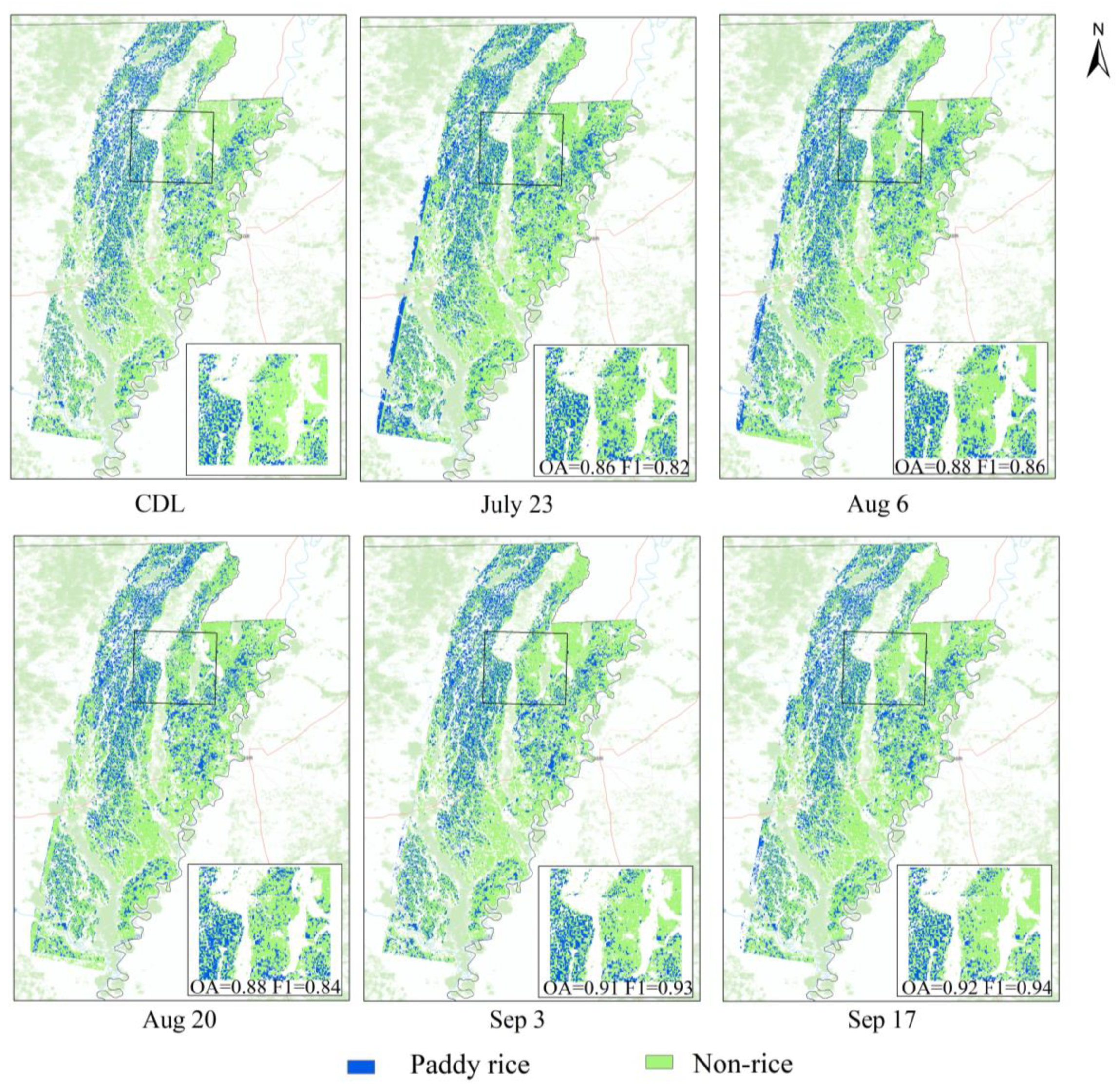
4.3.3. Dynamic Extraction of Paddy Rice

By inputting a single-date image separately for training and testing, it can be known that the extraction results of different dates are different. A total of 24 training experiments were conducted, each time the training samples were the datasets from 2017–2019, the number of training samples was the same, and the test year was 2020. The results show that in the test area (Figure 11), the extraction of a single image from 1–12 weeks (vegetative growth stage) (light green part in Figure 11) is not optimistic, and the extraction accuracy fluctuates greatly. From 13–18 weeks (reproductive growth stage) (dark green part in Figure 11), the extraction accuracy of rice rises except for the 17th week. From the end of the reproductive growth stage to the mature harvest stage (17–21 weeks), the extraction accuracy gradually improves and is highest at the 21st week, overall accuracy is 0.88, and the F1 score is 0.93.
According to the analysis in Section 4.3.2, we found that training data from multiple years from 2015–2019 was sufficient for the length of time and effective to identify paddy rice. Therefore, we used time series data from 2015–2019 with a fourteen-day interval and three bands to determine how accurate dynamic mapping can be.
The 15th week of 2020 (April 16) was set as the starting date with the ending date changing from the 21st week to the 37th week successively. All data between the starting date and ending date was used to perform rice extraction. In Figure 12, the x-axis represents the mapping date, the left y-axis refers to F1 scores. The extraction accuracy becomes higher with growing and surpasses 0.8 at the 29th week (July 23). Associated with the rice growing progress, paddy rice is at the heading stage (mid-July). The F1 score reaches 0.9 firstly at the 35th week (September 3) when part of the rice has entered the harvest period (early September).
5000 pixels of each class of sample were randomly selected, and the features of the two classes were extracted through the U-net and visualized by t-SNE. As reported in Figure 13, each figure corresponds to each period in Figure 12. It can be seen that with the extension of the time series, the separability of the sample features of each class increases, the “rice” class is gradually distinguished from the “non-rice” class, and the range of aggregation increases, which is consistent with the accuracy analysis results.

4.3.4. Dynamic Mapping and Comparison between the Paddy Rice Mapped and Statistical Data

Through the trained model, we can input the time series data of any year to generate the corresponding rice map. According to practical needs, users can input time series data of different time spans to obtain a dynamic distribution map of rice. The dynamic maps of paddy rice in 2020 was produced (Figure 14). The maps show the spatial distribution of paddy rice in the study area. The visual impression and accuracy of the mapping are affected by the quality of the RS images in the target year (the number of cloudless images and the amount of cloud in each RS image). The less cloud, the higher the integrity of the map. The historical images constitute a universal sample set allowing us to map paddy rice from Landsat images acquired in this area without additional ad hoc training sample collection. Therefore, an accurate and timely crop-type map provides estimations of the planting/harvesting crop areas for a variety of monitoring and decision-making applications.
We summed the rice paddy areas of ten counties in 2020 and compared them with the rice paddy planting area in 2020 from the USDA statistical data (https://quickstats.nass.usda.gov/, accessed on 21 May 2021) (Figure 15a). There is a significant linear relationship (r2 = 0.92) between the mapped area in the end-season derived from our results and those from the statistical reports (Figure 15b). Compared with end-season mapping, early-season mapping on 23 July overestimates the rice area.

5. Discussion

5.1. Comparison with Other Crop Extraction Studies

With the increase in the number of satellites and the improvement of spatial and temporal resolution, there have been many studies on rice extraction and rice mapping [20,31,56]. In recent years, deep learning, driven by remote sensing data, has been used for field crop remote sensing classification [30,41,57,58,59]. This study adopted a pixel-level end-to-end semantic segmentation model to extract rice. The extraction accuracy in the test area showed that the overall accuracy and F1 score are higher than those of the random forest model, which indicates that the deep learning model has learned both temporal features and spatial features. Compared with traditional machine learning models, it fully extracts the spectral features of different crops, enhances the separability, and is more suitable for the task of extracting rice based on time series data [60]. Using traditional machine learning methods to extract rice often requires sufficient prior knowledge and a large number of manually drawn samples [61], while the method proposed in this paper does not need to collect ground samples of the year. The time series images of rice can be automatically extracted, and the dynamic map of rice can be obtained in time.

5.2. The Choice of Time Interval and Band Combination

Time series data has become the main data type for crop classification. This paper conducts experiments and shows that time series data is more effective in rice extraction than a single image, and this conclusion has been confirmed in many studies [11,14,62]. Selecting appropriate time intervals is the key to construct time series data. It is useful to narrow the time interval of time series to capture key phenological information; however, making it too narrow will result in more missing data (due to cloud cover) [21,40]. As this study concludes, the model’s accuracy decreases when the time interval is twenty-eight days. This may be due to the small number of images or ignoring the temporal changes from the panicle initiation to the heading stage, which is a key physiological feature. This paper concludes that a fourteen-day time interval is more appropriate, which has also been reported by previous studies [21,40]. The extraction accuracy of rice in the key phenological period is relatively unstable. The absence of cloud-free images, climate change, or human activities causing the phenological period to move forward or backward may cause fluctuations in the extraction accuracy [8,21,63,64].
Multispectral and hyperspectral data have been used for crop classification. The features inputted into the model are high-dimensional and significant, which requires high demands on computing power [23]. Band selection reduces the dimensionality of the data without losing important information. Therefore, in this study, the Optimal Index Factor is used to remove repeated and low availability bands, and only the most effective bands for rice extraction are retained. The accuracies of rice extraction using the red, near-infrared, and short-wave infrared bands do not decrease much compared with the 6-band. This shows that these bands have a greater contribution to rice extraction, and some studies have also confirmed that near-infrared and short-wave infrared bands play an important role in the identification of rice and other crops [21,22,41].

5.3. Application of Dynamic Maps of Paddy Rice

Dynamic maps of rice are of high value to ensure grain security and agriculture production. The timely information is helpful to monitor crop growth status, to estimate crop yield. Wang et al. [65] reported that the booting stage was regarded as the optimal growth stage for rice yield estimation. Rice information extraction provides a more valuable base map for the cold damage risk assessment of agricultural meteorological disasters, which can happen in the early development of rice [66]. The identification of flood-affected rice paddies is essential for mitigating flood events, reducing property damage, and ensuring food security [67]. In addition, when drought, high temperature, typhoon, and other climate phenomena occur, rice mapping plays an important fundamental role to support mitigation and disaster response strategies in the region [68,69,70].
This study takes advantage of the deep learning model in processing time series data to fully learn the spectral and phenological temporal changes of early-growing rice, and preliminarily achieves the goal of dynamic mapping. The results show that the extraction accuracy of rice at the heading stage reaches more than 0.8, and it can reach 0.9 after the maturation stage. Some studies have reached similar conclusions when extracting other crop types [41,71,72]. It has become a common conclusion to use the transplanting period as the key identification period of rice [4,21], but when the remote sensing data of the transplanting period is missing, the accurate mapping of rice faces challenges. In this study, we conclude that the heading stage can be a key identification period for rice. Timely rice identification can be carried out approximately two months before maturation.

6. Conclusions

In this paper, we studied the potential of time series Landsat with a semantic segmentation model for paddy rice extraction and mapping. We proposed to use Landsat Level-2 products with the help of CDL as the ground truth in the field of crop mapping. Several key conclusions were drawn as follows:
  • The end-to-end semantic segmentation model outperformed the traditional classifier Random Forest for multi-temporal remote sensing data;
  • The band combination including red band, near-infrared band, and Swir-1 band could identify rice and decreased the training time compared with using all bands from Landsat;
  • The time interval of fourteen days could better capture the spectral characteristics of rice. A clear increase in performance occurred when more years of data were included with the performance increase plateauing after approximately five years;
  • During early rice paddy growth, the heading phase was proven to be an important time window for rice mapping. The overall accuracy and F1 score of the rice paddy planting area were 0.86 and 0.82, respectively.

Author Contributions

Conceptualization, M.D., P.W. and J.H.; methodology, M.D., P.W. and D.C.; software, M.D.; validation, M.D.; formal analysis, M.D., P.W., D.P. and W.S.; resources, M.D.; data curation, M.D.; writing—original draft preparation, M.D.; writing—review and editing, M.D., L.Y., R.H. and D.C.; visualization, M.D.; supervision, R.H. and J.H.; project administration, J.H., J.S. and R.H.; funding acquisition, J.H. and R.H. All authors have read and agreed to the published version of the manuscript.

Funding

This research was funded by the National Natural Science Foundation of China, grant number 42171314, 42101364 and Eramus+ Programme of the European Union, grant number 598838-EPP-1-2018-ELEPPKA2-CBHE-JP.

Data Availability Statement

The data presented in this study are available upon request from the corresponding author.

Conflicts of Interest

The authors declare no conflict of interest.

References

  1. Kuenzer, C.; Knauer, K. Remote sensing of rice crop areas. Int. J. Remote Sens. 2012, 34, 2101–2139. [Google Scholar] [CrossRef]
  2. Kim, M.K.; Tejeda, H.; Yu, T.E.U.S. milled rice markets and integration across regions and types. Int. Food Agribus. Manag. Rev. 2017, 20, 623–636. [Google Scholar] [CrossRef]
  3. Qin, Y.W.; Xiao, X.M.; Dong, J.W.; Zhou, Y.; Zhu, Z.; Zhang, G.; Du, G.; Jin, C.; Kou, W.; Wang, J.; et al. Mapping paddy rice planting area in cold temperate climate region through analysis of time series Landsat 8 (OLI), Landsat 7 (ETM+) and MODIS imagery. ISPRS J. Photogramm. Remote Sens. 2015, 105, 220–233. [Google Scholar] [CrossRef] [PubMed] [Green Version]
  4. Dong, J.W.; Xiao, X.M.; Menarguez, M.A.; Zhang, G.; Qin, Y.; Thau, D.; Biradar, C.; Moore, B. Mapping paddy rice planting area in northeastern Asia with Landsat 8 images, phenology-based algorithm and Google Earth Engine. Remote Sens. Environ. 2016, 185, 142–154. [Google Scholar] [CrossRef] [Green Version]
  5. Zhou, Y.T.; Xiao, X.M.; Qin, Y.W.; Dong, J.; Zhang, G.; Kou, W.; Jin, C.; Wang, J.; Li, X. Mapping paddy rice planting area in rice-wetland coexistent areas through analysis of Landsat 8 OLI and MODIS images. Int. J. Appl. Earth Obs. Geoinf. 2016, 46, 1–12. [Google Scholar] [CrossRef] [Green Version]
  6. Espe, M.B.; Cassman, K.G.; Yang, H.; Guilpart, N.; Grassini, P.; Van Wart, J.; Anders, M.; Beighley, D.; Harrell, D.; Linscombe, S.; et al. Yield gap analysis of US rice production systems shows opportunities for improvement. Field Crops Res. 2016, 196, 276–283. [Google Scholar] [CrossRef] [Green Version]
  7. FAO; IFAD; UNICEF; WFP; WHO. The State of Food Security and Nutrition in the World 2020; Food and Agriculture Organization of the United Nations: Rome, Italy, 2020; ISBN 978-92-5-132901-6. [Google Scholar]
  8. Dong, J.W.; Xiao, X.M. Evolution of regional to global paddy rice mapping methods: A review. ISPRS J. Photogramm. Remote Sens. 2016, 119, 214–227. [Google Scholar] [CrossRef] [Green Version]
  9. Liu, L.; Xiao, X.M.; Qin, Y.W.; Wang, J.; Xu, X.; Hu, Y.; Qiao, Z. Mapping cropping intensity in China using time series Landsat and Sentinel-2 images and Google Earth Engine. Remote Sens. Environ. 2020, 239, 111624. [Google Scholar] [CrossRef]
  10. Gandharum, L.; Mulyani, M.E.; Hartono, D.M.; Karsidi, A.; Ahmad, M. Remote sensing versus the area sampling frame method in paddy rice acreage estimation in Indramayu regency, West Java province, Indonesia. Int. J. Remote Sens. 2020, 42, 1738–1767. [Google Scholar] [CrossRef]
  11. Rawat, A.; Kumar, A.; Upadhyay, P.; Kumar, S. Deep learning-based models for temporal satellite data processing: Classification of paddy transplanted fields. Ecol. Inform. 2021, 61, 101214. [Google Scholar] [CrossRef]
  12. Gusso, A.; Guo, W.; Rolim, S.B.A. Reflectance-based model for soybean mapping in United States at common land unit scale with Landsat 8. Eur. J. Remote Sens. 2019, 52, 522–531. [Google Scholar] [CrossRef] [Green Version]
  13. Jin, C.; Xiao, X.M.; Dong, J.W.; Qin, Y.; Wang, Z. Mapping paddy rice distribution using multi-temporal Landsat imagery in the Sanjiang Plain, northeast China. Front. Earth Sci. 2016, 10, 49–62. [Google Scholar] [CrossRef] [PubMed] [Green Version]
  14. Xu, J.F.; Zhu, Y.; Zhong, R.H.; Lin, Z.X.; Xu, J.; Jiang, H.; Huang, J.; Li, H.; Lin, T. DeepCropMapping: A multi-temporal deep learning approach with improved spatial generalizability for dynamic corn and soybean mapping. Remote Sens. Environ. 2020, 247, 111946. [Google Scholar] [CrossRef]
  15. Zhu, Z.; Woodcock, C.E. Continuous change detection and classification of land cover using all available Landsat data. Remote Sens. Environ. 2014, 144, 152–171. [Google Scholar] [CrossRef] [Green Version]
  16. Inglada, J.; Arias, M.; Tardy, B.; Hagolle, O.; Valero, S.; Morin, D.; Dedieu, G.; Sepulcre, G.; Bontemps, S.; Defourny, P.; et al. Assessment of an operational system for crop type map production using high temporal and spatial resolution satellite optical imagery. Remote Sens. 2015, 7, 12356–12379. [Google Scholar] [CrossRef] [Green Version]
  17. Xiao, X.M.; Boles, S.; Liu, J.Y.; Zhuang, D.; Frolking, S.; Li, C.; Salas, W.; Moore, B. Mapping paddy rice agriculture in southern China using multi-temporal MODIS images. Remote Sens. Environ. 2005, 95, 480–492. [Google Scholar] [CrossRef]
  18. Singha, M.; Wu, B.F.; Zhang, M. Object-based paddy rice mapping using HJ-1A/B data and temporal features extracted from time series MODIS NDVI data. Sensors 2016, 17, 10. [Google Scholar] [CrossRef] [Green Version]
  19. Wardlow, B.D.; Egbert, S.L. Large-area crop mapping using time-series MODIS 250 m NDVI data: An assessment for the U.S. Central Great Plains. Remote Sens. Environ. 2008, 112, 1096–1116. [Google Scholar] [CrossRef]
  20. Yang, L.B.; Wang, L.M.; Abubakar, G.A.; Huang, J. High-resolution rice mapping based on SNIC segmentation and multi-source remote sensing images. Remote Sens. 2021, 13, 1148. [Google Scholar] [CrossRef]
  21. You, N.S.; Dong, J.W. Examining earliest identifiable timing of crops using all available Sentinel 1/2 imagery and Google Earth Engine. ISPRS J. Photogramm. Remote Sens. 2020, 161, 109–123. [Google Scholar] [CrossRef]
  22. Hao, P.Y.; Zhan, Y.L.; Wang, L.; Niu, Z.; Shakir, M. Feature selection of time series MODIS data for early crop classification using Random Forest: A case study in Kansas, USA. Remote Sens. 2015, 7, 5347–5369. [Google Scholar] [CrossRef] [Green Version]
  23. Pelletier, C.; Valero, S.; Inglada, J.; Champion, N.; Dedieu, G. Assessing the robustness of Random Forests to map land cover with high resolution satellite image time series over large areas. Remote Sens. Environ. 2016, 187, 156–168. [Google Scholar] [CrossRef]
  24. Chen, C.F.; Son, N.T.; Chen, C.R.; Chang, L.Y. Wavelet filtering of time-series moderate resolution imaging spectroradiometer data for rice crop mapping using support vector machines and maximum likelihood classifier. Med. Eng. Phys. 2011, 5, 3525. [Google Scholar] [CrossRef]
  25. Ghassemi, B.; Dujakovic, A.; Zoltak, M.; Immitzer, M.; Atzberger, C.; Vuolo, F. Designing a European-wide crop type mapping approach based on machine learning algorithms using LUCAS field survey and Sentinel-2 data. Remote Sens. 2022, 14, 541. [Google Scholar] [CrossRef]
  26. Son, N.T.; Chen, C.F.; Chen, C.R.; Minh, V.Q. Assessment of Sentinel-1A data for rice crop classification using random forests and support vector machines. Geocarto Int. 2018, 33, 587–601. [Google Scholar] [CrossRef]
  27. Saini, R.; Ghosh, S.K. Crop classification in a heterogeneous agricultural environment using ensemble classifiers and single-date Sentinel-2A imagery. Geocarto Int. 2021, 36, 2141–2159. [Google Scholar] [CrossRef]
  28. Belgiu, M.; Csillik, O. Sentinel-2 cropland mapping using pixel-based and object-based time-weighted dynamic time warping analysis. Remote Sens. Environ. 2018, 204, 509–523. [Google Scholar] [CrossRef]
  29. Wei, P.L.; Chai, D.F.; Lin, T.; Tang, C.; Du, M.; Huang, J. Large-scale rice mapping under different years based on time-series Sentinel-1 images using deep semantic segmentation model. ISPRS J. Photogramm. Remote Sens. 2021, 174, 198–214. [Google Scholar] [CrossRef]
  30. Du, Z.R.; Yang, J.Y.; Ou, C.; Zhang, T. Smallholder crop area mapped with a semantic segmentation deep learning method. Remote Sens. 2019, 11, 888. [Google Scholar] [CrossRef] [Green Version]
  31. Zhang, W.C.; Liu, H.B.; Wu, W.; Zhan, L.; Wei, J. Mapping rice paddy based on machine learning with Sentinel-2 multi-temporal data: Model comparison and transferability. Remote Sens. 2020, 12, 1620. [Google Scholar] [CrossRef]
  32. Ding, J.; Chen, B.; Liu, H.W.; Huang, M. Convolutional neural network with data augmentation for SAR target recognition. IEEE Geosci. Remote Sens. Lett. 2016, 13, 1–5. [Google Scholar] [CrossRef]
  33. Ji, S.P.; Zhang, Z.L.; Zhang, C.; Wei, S.; Lu, M.; Duan, Y. Learning discriminative spatiotemporal features for precise crop classification from multi-temporal satellite images. Int. J. Remote Sens. 2019, 41, 3162–3174. [Google Scholar] [CrossRef]
  34. Li, F.; Zhang, C.M.; Zhang, W.W.; Xu, Z.; Wang, S.; Sun, G.; Wang, Z. Improved winter wheat spatial distribution extraction from high-resolution remote sensing imagery using semantic features and statistical analysis. Remote Sens. 2020, 12, 538. [Google Scholar] [CrossRef] [Green Version]
  35. Hajj, M.E.; Baghdadi, N.; Zribi, M.; Bazzi, H. Synergic use of Sentinel-1 and Sentinel-2 images for operational soil moisture mapping at high spatial resolution over agricultural areas. Remote Sens. 2017, 9, 1292. [Google Scholar] [CrossRef] [Green Version]
  36. Boryan, C.; Yang, Z.; Mueller, R.; Craig, M. Monitoring US agriculture: The US department of agriculture, national agricultural statistics service, Cropland Data Layer program. Geocarto Int. 2011, 26, 341–358. [Google Scholar] [CrossRef]
  37. Ronneberger, O.; Fischer, P.; Brox, T. U-net: Convolutional networks for biomedical image segmentation. In Proceedings of the International Conference on Medical Image Computing and Computer-Assisted Intervention, Munich, Germany, 5–9 October 2015; Springer: Berlin/Heidelberg, Germany, 2015. [Google Scholar]
  38. Zhong, L.H.; Hu, L.N.; Zhou, H. Deep learning based multi-temporal crop classification. Remote Sens. Environ. 2019, 221, 430–443. [Google Scholar] [CrossRef]
  39. Wang, J.; Xiao, X.M.; Liu, L.; Wu, X.; Qin, Y.; Steiner, J.L.; Dong, J. Mapping sugarcane plantation dynamics in Guangxi, China, by time series Sentinel-1, Sentinel-2 and Landsat images. Remote Sens. Environ. 2020, 247, 111951. [Google Scholar] [CrossRef]
  40. Griffiths, P.; Nendel, C.; Hostert, P. Intra-annual reflectance composites from Sentinel-2 and Landsat for national-scale crop and land cover mapping. Remote Sens. Environ. 2019, 220, 135–151. [Google Scholar] [CrossRef]
  41. Cai, Y.P.; Guan, K.Y.; Peng, J.; Wang, S.; Seifert, C.; Wardlow, B.; Li, Z. A high-performance and in-season classification system of field-level crop types using time-series Landsat data and a machine learning approach. Remote Sens. Environ. 2018, 210, 35–47. [Google Scholar] [CrossRef]
  42. Motschenbacher, J.M.; Brye, K.R.; Anders, M.M.; Gbur, E.E.; Slaton, N.A.; Evans-White, M.A. Daily soil surface CO2 flux during non-flooded periods in flood-irrigated rice rotations. Agron. Sustain. Dev. 2014, 35, 771–782. [Google Scholar] [CrossRef] [Green Version]
  43. Brouwer, C.; Prins, K.; Heibloem, M. Irrigation Water Management: Irrigation Scheduling; Training manual No. 4; FAO: Rome, Italy, 1989. [Google Scholar]
  44. Chavez, P.S.; Berlin, G.L.; Sowers, L.B. Statistical-method for selecting Landsat MSS ratios. J. Appl. Photogr. Eng. 1982, 8, 23–30. [Google Scholar]
  45. Long, J.; Shelhamer, E.; Darrell, T. Fully Convolutional Networks for Semantic Segmentation. IEEE Trans. Pattern Anal. Mach. Intell. 2015, 39, 640–651. [Google Scholar]
  46. Chai, D.F.; Newsam, S.; Zhang, H.K.; Qiu, Y.F.; Huang, J. Cloud and cloud shadow detection in Landsat imagery based on deep convolutional neural networks. Remote Sens. Environ. 2019, 225, 307–316. [Google Scholar] [CrossRef]
  47. Waldner, F.; Diakogiannis, F.I. Deep learning on edge: Extracting field boundaries from satellite images with a convolutional neural network. Remote Sens. Environ. 2020, 245, 111741. [Google Scholar] [CrossRef]
  48. Breiman, L. Random Forests. Mach. Learn. 2001, 45, 5–32. [Google Scholar] [CrossRef] [Green Version]
  49. Zhao, Y.Y.; Feng, D.L.; Yu, L.; Wang, X.Y.; Chen, Y.; Bai, Y.; Hernández, H.J.; Galleguillos, M.; Estades, C.; Biging, G.S.; et al. Detailed dynamic land cover mapping of Chile: Accuracy improvement by integrating multi-temporal data. Remote Sens. Environ. 2016, 183, 170–185. [Google Scholar] [CrossRef]
  50. Belgiu, M.; Stein, A. Spatiotemporal image fusion in Remote Sensing. Remote Sens. 2019, 11, 818. [Google Scholar] [CrossRef] [Green Version]
  51. Rodriguez-Galiano, V.F.; Chica-Olmo, M.; Abarca-Hernandez, F.; Atkinson, P.M.; Jeganathan, C. Random Forest classification of Mediterranean land cover using multi-seasonal imagery and multi-seasonal texture. Remote Sens. Environ. 2012, 121, 93–107. [Google Scholar] [CrossRef]
  52. Van der Maaten, L.; Hinton, G. Visualizing data using t-SNE. J. Mach. Learn. Res. 2008, 9, 2579–2605. [Google Scholar]
  53. Son, N.T.; Chen, C.F.; Chen, C.R.; Duc, H.N.; Chang, L.Y. A phenology-based classification of time-series MODIS data for rice crop monitoring in Mekong Delta, Vietnam. Remote Sens. 2013, 6, 135–156. [Google Scholar] [CrossRef] [Green Version]
  54. Ding, M.J.; Guan, Q.H.; Li, L.H.; Zhang, H.; Liu, C.; Zhang, L. Phenology-based rice paddy mapping using multi-source satellite imagery and a fusion algorithm applied to the Poyang Lake Plain, Southern China. Remote Sens. 2020, 12, 1022. [Google Scholar] [CrossRef] [Green Version]
  55. Linquist, B.A.; Marcos, M.; Adviento-Borbe, M.A.; Anders, M.; Harrell, D.; Linscombe, S.; Reba, M.L.; Runkle, B.R.K.; Tarpley, L.; Thomson, A. Greenhouse Gas Emissions and Management Practices that Affect Emissions in US Rice Systems. J. Environ. Qual. 2018, 47, 395–409. [Google Scholar] [CrossRef] [PubMed] [Green Version]
  56. Yang, H.J.; Pan, B.; Wu, W.F.; Tai, J. Field-based rice classification in Wuhua county through integration of multi-temporal Sentinel-1A and Landsat-8 OLI data. Int. J. Appl. Earth Obs. Geoinf. 2018, 69, 226–236. [Google Scholar] [CrossRef]
  57. Su, D.; Kong, H.; Qiao, Y.L.; Sukkarieh, S. Data augmentation for deep learning based semantic segmentation and crop-weed classification in agricultural robotics. Comput. Electron. Agric. 2021, 190, 106418. [Google Scholar] [CrossRef]
  58. Giannopoulos, M.; Tsagkatakis, G.; Tsakalides, P. 4D U-Nets for multi-temporal remote sensing data classification. Remote Sens. 2022, 14, 634. [Google Scholar] [CrossRef]
  59. Boulila, W.; Sellami, M.; Driss, M.; Al-Sarem, M.; Safaei, M.; Ghaleb, F.A. RS-DCNN: A novel distributed convolutional-neural-networks based-approach for big remote-sensing image classification. Comput. Electron. Agric. 2021, 182, 106014. [Google Scholar] [CrossRef]
  60. Yaramasu, R.; Bandaru, V.; Pnvr, K. Pre-season crop type mapping using deep neural networks. Comput. Electron. Agric. 2020, 176, 105664. [Google Scholar] [CrossRef]
  61. Li, H.; Fu, D.J.; Huang, C.; Su, F.Z.; Liu, Q.S.; Liu, G.H.; Wu, S. An approach to high-resolution rice paddy mapping using time-series Sentinel-1 SAR data in the Mun River Basin, Thailand. Remote Sens. 2020, 12, 3959. [Google Scholar] [CrossRef]
  62. Vuolo, F.; Neuwirth, M.; Immitzer, M.; Atzberger, C.; Ng, W.-T. How much does multi-temporal Sentinel-2 data improve crop type classification? Int. J. Appl. Earth Obs. Geoinf. 2018, 72, 122–130. [Google Scholar] [CrossRef]
  63. Yuan, Q.Q.; Shen, H.F.; Li, T.W.; Li, Z.; Li, S.; Jiang, Y.; Xu, H.; Tan, W.; Yang, Q.; Wang, J.; et al. Deep learning in environmental remote sensing: Achievements and challenges. Remote Sens. Environ. 2020, 241, 111716. [Google Scholar] [CrossRef]
  64. Ozdogan, M.; Yang, Y.; Allez, G.; Cervantes, C. Remote sensing of irrigated agriculture: Opportunities and challenges. Remote Sens. 2010, 2, 2274–2304. [Google Scholar] [CrossRef] [Green Version]
  65. Wang, F.L.; Wang, F.M.; Zhang, Y.; Hu, J.H.; Huang, J.F.; Xie, J.K. Rice yield estimation using Parcel-Level relative spectra variables from UAV-based hyperspectral imagery. Front. Plant Sci. 2019, 10, 453. [Google Scholar] [CrossRef] [PubMed] [Green Version]
  66. Cheng, Y.X.; Huang, J.F.; Han, Z.L.; Guo, J.P.; Zhao, Y.X.; Wang, X.Z.; Guo, R.F. Cold damage risk assessment of Double Cropping Rice in Hunan, China. J. Integr. Agric. 2013, 12, 352–363. [Google Scholar] [CrossRef]
  67. Singha, M.; Dong, J.W.; Sarmah, S.; You, N.S.; Zhou, Y.; Zhang, G.L.; Doughty, R.; Xiao, X.M. Identifying floods and flood-affected paddy rice fields in Bangladesh based on Sentinel-1 imagery and Google Earth Engine. ISPRS J. Photogramm. Remote Sens. 2020, 166, 278–293. [Google Scholar] [CrossRef]
  68. Zhang, G.; Zhang, S.; Wang, L.; Xiao, Y.; Tang, W.; Chen, G.; Chen, L. Effects of high temperature at different times during the heading and filling periods on rice quality. Sci. Agric. Sin. 2013, 46, 2869–2879. [Google Scholar]
  69. Boschetti, M.; Nelson, A.; Nutini, F.; Manfron, G.; Busetto, L.; Barbieri, M.; Laborte, A.; Raviz, J.; Holecz, F.; Mabalay, M.R.O.; et al. Rapid assessment of crop status: An application of MODIS and SAR data to rice areas in Leyte, Philippines affected by typhoon Haiyan. Remote Sens. 2015, 7, 6535–6557. [Google Scholar] [CrossRef] [Green Version]
  70. Fu, X.; Zhao, G.N.; Wu, W.C.; Xu, B.; Li, J.; Zhou, X.T.; Ke, X.X.; Li, Y.; Li, W.J.; Zhou, C.M.; et al. Assessing the impacts of natural disasters on rice production in Jiangxi, China. Int. J. Remote Sens. 2022, 43, 1919–1941. [Google Scholar] [CrossRef]
  71. Skakun, S.; Franch, B.; Vermote, E.; Roger, J.C.; Becker-Reshef, I.; Justice, C.; Kussul, N. Early season large-area winter crop mapping using MODIS NDVI data, growing degree days information and a Gaussian mixture model. Remote Sens. Environ. 2017, 195, 244–258. [Google Scholar] [CrossRef]
  72. McNairn, H.; Kross, A.; Lapen, D.; Caves, R.; Shang, J. Early season monitoring of corn and soybeans with TerraSAR-X and RADARSAT-2. Int. J. Appl. Earth Obs. Geoinf. 2014, 28, 252–259. [Google Scholar] [CrossRef]
Figure 1. (a) Location of Arkansas. (b) Crop types of Arkansas in 2018. (c) Training and test area. The gray represents the coverage of Landsat image tiles. AR: Arkansas; MO: Missouri; OK: Oklahoma; TX: Texas; LA: Louisiana; MS: Mississippi; TN: Tennessee; KY: Kentucky; IL: Illinois.
Agronomy 12 01583 g001
Figure 2. Temporal distribution of Landsat 8 and Landsat 7 images used in this study. (a) path/row 23/35; (b) path/row 23/36.
Agronomy 12 01583 g002
Figure 3. The progress of rice paddy life cycle from 2015–2020 according to USDA data. The Y-axis includes progress measured in PCT planted (PCT planted), progress measured in PCT emerged (PCT emerged), and progress measured in PCT harvested (PCT harvested). The X-axis is calculated from the first week of each year. The gray area represents the research span of time, for which the starting data starts from the PCT emerged.
Agronomy 12 01583 g003
Figure 4. Network structure. It was built based on U-Net, including encoder and decoder. After inputting images of different bands, the net can output rice extraction images with the same spatial resolution.
Agronomy 12 01583 g004
Figure 5. Seasonal profiles of spectral reflectance of paddy rice, soybean, and “other” pixels from 2017 to 2019. The buffers indicate one standard deviation calculated from all fields and years. The X-axis represents research span (a total of 24 weeks) and the Y-axis is the value of reflectance. The blue lines represent the average values of paddy rice, the green lines represent the average values of soybeans, and the orange lines represent the average values of “other”. (a) Blue band. (b) Green band. (c) Red band. (d) Nir band. (e) Swir-1 band. (f) Swir-2 band.
Agronomy 12 01583 g005
Figure 6. Rice extraction results of test area in 2020 for U-net and Random Forest classifiers with different time interval scenarios. (a) Overall accuracy; (b) F1 scores.
Agronomy 12 01583 g006
Figure 7. The effect of band selection on the extraction accuracy. The 3-band combination includes red band, near-infrared band, and Swir-1 band. The 6-band combination includes red, green, blue, near-infrared, and two Swir bands. (a) Overall accuracy; (b) F1 scores; (c) Training time.
Agronomy 12 01583 g007
Figure 8. Visualization of inputted features and extracted features by model with different time intervals and band combinations. The 3-band combination includes red band, near-infrared band, and Swir-1 band. The 6-band combination includes red, green, blue, near-infrared, and two Swir bands.
Agronomy 12 01583 g008
Figure 9. Extraction accuracies based on training samples of multiple years. (a) Using the data (with time interval of 28 days) of different numbers of continuous years ending in 2019 to predict crop types in 2020; (b) Using the data (with time interval of 14 days) of different numbers of continuous years ending in 2019 to predict crop types in 2020.
Agronomy 12 01583 g009
Figure 10. Extraction accuracies based on training samples from 2013–2017. (a) Overall accuracy; (b) F1 scores.
Agronomy 12 01583 g010
Figure 11. Extraction results of single remote sensing image, where overall accuracy (OA) is a histogram, and F1 score(F1) is a line graph. The X-axis represent research span of time (a total of 24 weeks).
Agronomy 12 01583 g011
Figure 12. Accuracies of dynamic mapping (F1 scores) of paddy rice as the length of the time series increasing, which started from 16 April 2020 (light green is the vegetative phase, dark green is the reproductive phase, and orange is the ripening phase).
Agronomy 12 01583 g012
Figure 13. Visualization of features extracted on different mapping date as the length of the time series increasing, which started from 16 April 2020.
Agronomy 12 01583 g013
Figure 14. The dynamic maps of paddy rice in 2020 (Spatial resolution is 30 m). Time series starts on 16 April and the date represents the mapping date.
Agronomy 12 01583 g014
Figure 15. A comparison of paddy rice area estimates by 10 counties between the rice paddy map in 2020 and the statistical data reported in 2020. This comparison used the linear regression model of y = a × x + b. The end-season map was made on 17 September. The early-season map was made on 23 July. (a) Area statistics histogram. (b) A comparison of paddy rice area estimates between mapping and statistics.
Agronomy 12 01583 g015
Table 1. The correlation coefficient matrix between each band (the shaded part is the result of masking non-rice pixels).
BlueGreenRedNirSwir-1Swir-2
Blue10.9730.9730.1590.8310.903
Green0.97710.9740.2660.8220.878
Red0.9710.98910.1390.8400.906
Nir0.8240.8720.84710.4510.294
Swir-10.8870.8630.8740.85910.964
Swir-20.9060.8690.8800.7800.9781
Table 2. The OIF indexes corresponding to all possible band combinations.
Blue/Nir/Swir-1Blue /Nir/Swir-2Green/Nir/Swir-1Green/Nir/Swir-2Red/Nir/Swir-1Red/Nir/Swir-2
All pixelsOIF7069.66730.27266.56932.17433.47080.2
Rice pixelsOIF4305.34088.54438.34221.64537.34320.1
Publisher’s Note: MDPI stays neutral with regard to jurisdictional claims in published maps and institutional affiliations.

