
Tender Leaf Identification for Early-Spring Green Tea Based on Semi-Supervised Learning and Image Processing


Abstract
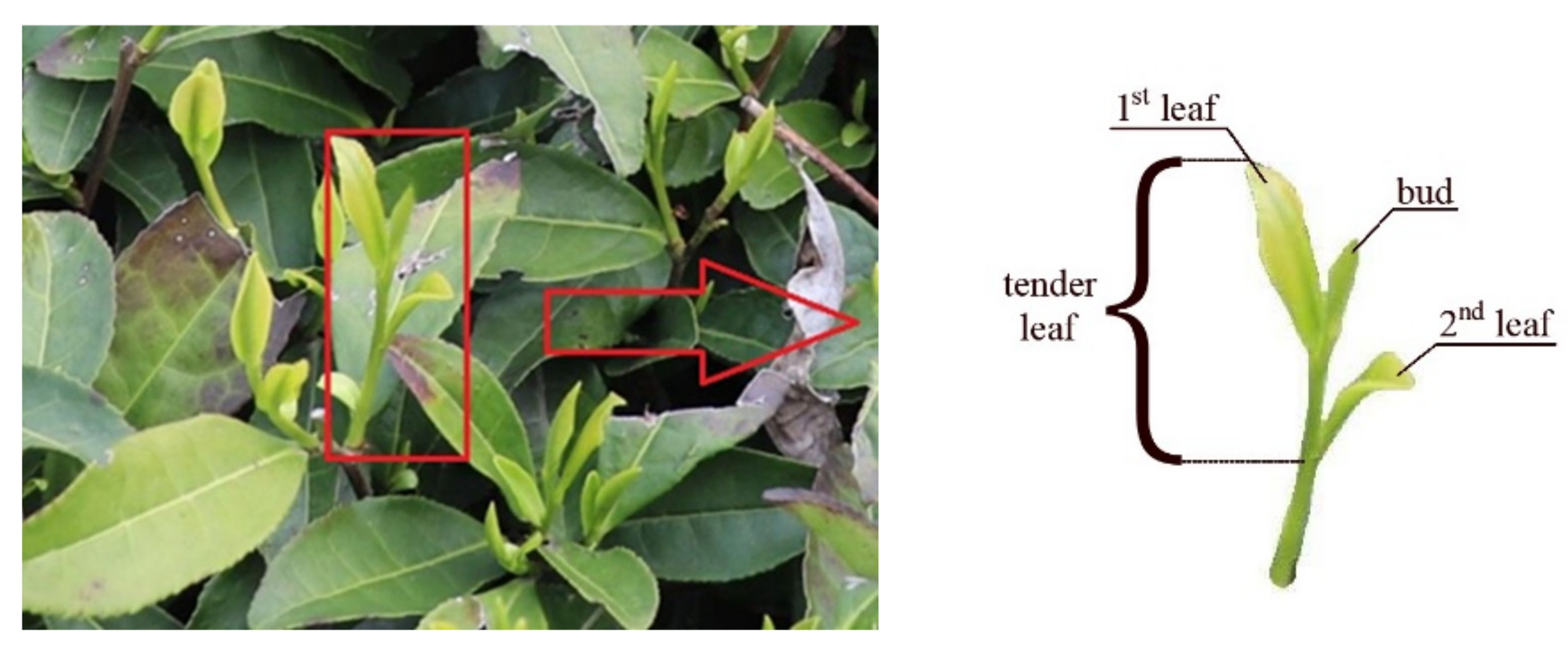
:1. Introduction
2. Materials and Methods
2.1. Image Acquisition
2.2. Training and Testing
2.2.1. Data Acquisition
2.2.2. Training and Testing in Two-Dimensional Space
2.2.3. Training and Testing in Three-Dimensional Space
2.3. Image Processing
3. Results and Discussion
3.1. Visualization and Objective Function in Two-Dimensional Space
3.2. Visualization and Objective Function in Three-Dimensional Space
3.3. Identification Result on Tender Leaves
4. Conclusions
Author Contributions
Funding
Institutional Review Board Statement
Informed Consent Statement
Data Availability Statement
Acknowledgments
Conflicts of Interest
References
- Graham, H.N. Green tea composition, consumption, and polyphenol chemistry. Prev. Med. 1992, 21, 334–350. [Google Scholar] [CrossRef]
- Liu, J.; Zhang, Q.; Liu, M.; Ma, L.; Shi, Y.; Ruan, J. Metabolomic Analyses Reveal Distinct Change of Metabolites and Quality of Green Tea during the Short Duration of a Single Spring Season. J. Agric. Food Chem. 2016, 64, 3302–3309. [Google Scholar] [CrossRef] [PubMed]
- Wang, J.; Zeng, X.; Liu, J. Three-Dimensional Modeling of Tea-Shoots Using Images and Models. Sensors 2011, 11, 3803–3815. [Google Scholar] [CrossRef] [PubMed]
- Tang, Z.; Su, Y.; Er, M.J.; Qi, F.; Zhang, L.; Zhou, J. A local binary pattern based texture descriptors for classification of tea leaves. Neurocomputing 2015, 168, 1011–1023. [Google Scholar] [CrossRef]
- Chen, J.; Chen, Y.; Jin, X.; Che, J.; Gao, F.; Li, N. Research on a Parallel Robot for Green Tea Flushes Plucking. In Proceedings of the 2015 International Conference on Education, Management, Information and Medicine, Shenyang, China, 24–26 April 2015; pp. 22–26. [Google Scholar]
- Zhang, L.; Zhang, H.; Chen, Y.; Dai, S.; Li, X.; Imou, K.; Liu, Z.; Li, M. Real-time monitoring of optimum timing for harvesting fresh tea leaves based on machine vision. Int. J. Agric. Biol. Eng. 2019, 12, 6–9. [Google Scholar] [CrossRef]
- Mukhopadhyay, S.; Paul, M.; Pal, R.; De, D. Tea leaf disease detection using multi-objective image segmentation. Multimed. Tools Appl. 2021, 80, 753–771. [Google Scholar] [CrossRef]
- De Marsico, M.; Petrosino, A.; Ricciardi, S. Iris recognition through machine learning techniques: A survey. Pattern Recognit. Lett. 2016, 82, 106–115. [Google Scholar] [CrossRef]
- Suto, J. Plant leaf recognition with shallow and deep learning: A comprehensive study. Intell. Data Anal. 2020, 24, 1311–1328. [Google Scholar] [CrossRef]
- Verbraken, T.; Verbeke, W.; Baesens, B. Profit optimizing customer churn prediction with Bayesian network classifiers. Intell. Data Anal. 2012, 18, 3–24. [Google Scholar] [CrossRef]
- Yamamoto, K.; Yoshioka, Y.; Ninomiya, S.; Culsp. Detection and counting of intact tomato fruits on tree using image analysis and machine learning methods. In Proceedings of the 5th International Conference, TAE 2013: Trends in Agricultural Engineering 2013, Prague, Czech Republic, 2–3 September 2013.
- Tripathi, M.K.; Maktedar, D.D. Recent machine learning based approaches for disease detection and classification of agricultural products. In Proceedings of the 2016 International Conference on Computing Communication Control and Automation (ICCUBEA), Pune, India, 12–13 August 2016; pp. 1–6. [Google Scholar]
- Zhao, Y.; Gong, L.; Zhou, B.; Huang, Y.; Liu, C. Detecting tomatoes in greenhouse scenes by combining AdaBoost classifier and colour analysis. Biosyst. Eng. 2016, 148, 127–137. [Google Scholar] [CrossRef]
- Kim, J.; Cho, W.; Na, M.; Chun, M. Development of Automatic Classification System of Vegetables by Image Processing and Deep Learning. J. Korean Data Anal. Soc. 2019, 21, 63–73. [Google Scholar] [CrossRef]
- Hu, G.; Wu, H.; Zhang, Y.; Wan, M. A low shot learning method for tea leaf’s disease identification. Comput. Electron. Agric. 2019, 163, 104852. [Google Scholar] [CrossRef]
- Nyalala, I.; Okinda, C.; Nyalala, L.; Makange, N.; Chao, Q.; Chao, L.; Yousaf, K.; Chen, K. Tomato volume and mass estimation using computer vision and machine learning algorithms: Cherry tomato model. J. Food Eng. 2019, 263, 288–298. [Google Scholar] [CrossRef]
- Sun, Y.; Jiang, Z.; Zhang, L.; Dong, W.; Rao, Y. SLIC_SVM based leaf diseases saliency map extraction of tea plant. Comput. Electron. Agric. 2019, 157, 102–109. [Google Scholar] [CrossRef]
- Xie, C.; Liu, Y.; Zeng, W.L.; Lu, X.B. An improved method for single image super-resolution based on deep learning. Signal Image Video P. 2019, 13, 557–565. [Google Scholar] [CrossRef]
- Fan, S.; Li, J.; Zhang, Y.; Tian, X.; Wang, Q.; He, X.; Zhang, C.; Huang, W. On line detection of defective apples using computer vision system combined with deep learning methods. J. Food Eng. 2020, 286, 110102. [Google Scholar] [CrossRef]
- Osako, Y.; Yamane, H.; Lin, S.-Y.; Chen, P.-A.; Tao, R. Cultivar discrimination of litchi fruit images using deep learning. Sci. Hortic. 2020, 269, 109360. [Google Scholar] [CrossRef]
- Duong, L.T.; Nguyen, P.T.; Di Sipio, C.; Di Ruscio, D. Automated fruit recognition using EfficientNet and MixNet. Comput. Electron. Agric. 2020, 171, 105326. [Google Scholar] [CrossRef]
- LeCun, Y.; Bengio, Y.; Hinton, G. Deep learning. Nature 2015, 521, 436. [Google Scholar] [CrossRef]
- Ni, C.; Wang, D.; Vinson, R.; Holmes, M.; Tao, Y. Automatic inspection machine for maize kernels based on deep convolutional neural networks. Biosyst. Eng. 2019, 178, 131–144. [Google Scholar] [CrossRef]
- Saood, A.; Hatem, I. COVID-19 lung CT image segmentation using deep learning methods: U-Net versus SegNet. BMC Med. Imag. 2021, 21, 19. [Google Scholar] [CrossRef]
- Geng, D.V.; Alkhachroum, A.; Bicchi, M.A.M.; Jagid, J.R.; Cajigas, I.; Chen, Z.S. Deep learning for robust detection of interictal epileptiform discharges. J. Neural Eng. 2021, 18, 056015. [Google Scholar] [CrossRef]
- Yao, P.; Gai, S.; Chen, Y.; Chen, W.; Da, F. A multi-code 3D measurement technique based on deep learning. Opt. Lasers Eng. 2021, 143, 106623. [Google Scholar] [CrossRef]
- Ma, J.S.; Sheridan, R.P.; Liaw, A.; Dahl, G.E.; Svetnik, V. Deep Neural Nets as a Method for Quantitative Structure-Activity Relationships. J. Chem Inf. Model. 2015, 55, 263–274. [Google Scholar] [CrossRef]
- Ciodaro, T.; Deva, D.; De Seixas, J.; Damazio, D. Online particle detection with Neural Networks based on topological calorimetry information. In Proceedings of the14th International Workshop on Advanced Computing and Analysis Techniques in Physics Research (ACAT), Brunel Univ, Uxbridge, UK, 5–9 September 2011; IOP Publishing: Bristol, UK, 2012; Volume 368. [Google Scholar]
- Azhari, M.; Abarda, A.; Ettaki, B.; Zerouaoui, J.; Dakkon, M. Higgs Boson Discovery using Machine Learning Methods with Pyspark. Procedia Comput. Sci. 2020, 170, 1141–1146. [Google Scholar] [CrossRef]
- Shi, J.; Li, Z.; Zhu, T.; Wang, D.; Ni, C. Defect detection of industry wood veneer based on NAS and multi-channel mask R-CNN. Sensors 2020, 20, 4398. [Google Scholar] [CrossRef]
- Zhou, H.; Zhuang, Z.; Liu, Y.; Liu, Y.; Zhang, X. Defect Classification of Green Plums Based on Deep Learning. Sensors 2020, 20, 6993. [Google Scholar] [CrossRef]
- Jin, X.; Bagavathiannan, M.; Maity, A.; Chen, Y.; Yu, J. Deep learning for detecting herbicide weed control spectrum in turfgrass. Plant Methods 2022, 18, 94. [Google Scholar] [CrossRef]
- Helmstaedter, M.; Briggman, K.L.; Turaga, S.C.; Jain, V.; Seung, H.S.; Denk, W. Connectomic reconstruction of the inner plexiform layer in the mouse retina. Nature 2013, 500, 168–174. [Google Scholar] [CrossRef]
- Bottou, L. Large-scale machine learning with stochastic gradient descent. In Proceedings of the COMPSTAT 2010, Paris, France, 22–27 August 2010; Springer: Berlin/Heidelberg, Germany, 2010; pp. 177–186. [Google Scholar]
- Liu, W.; Chen, L.; Chen, Y.; Zhang, W. Accelerating Federated Learning via Momentum Gradient Descent. IEEE Trans. Parallel Distrib. Syst. 2020, 31, 1754–1766. [Google Scholar] [CrossRef]
- Kingma, D.P.; Ba, J. Adam: A Method for Stochastic Optimization. 2014. Available online: https://arxiv.org/abs/1412.6980 (accessed on 30 January 2017).


| i | Training Accuracy | Training Loss | Testing Accuracy | Testing Loss |
|---|---|---|---|---|
| 0 | 0.500000 | 0.525362 | 0.500000 | 0.573693 |
| 100 | 1.000000 | 0.230712 | 1.000000 | 0.326605 |
| 200 | 1.000000 | 0.141746 | 0.995000 | 0.244365 |
| 300 | 1.000000 | 0.101258 | 0.995000 | 0.203138 |
| 400 | 1.000000 | 0.078506 | 0.995000 | 0.178050 |
| 500 | 1.000000 | 0.064027 | 0.995000 | 0.160973 |
| 600 | 1.000000 | 0.054032 | 0.990000 | 0.148480 |
| 700 | 1.000000 | 0.046729 | 0.990000 | 0.138872 |
| 800 | 1.000000 | 0.041164 | 0.990000 | 0.131209 |
| 900 | 1.000000 | 0.036786 | 0.990000 | 0.124924 |
| 1000 | 1.000000 | 0.033252 | 0.990000 | 0.119654 |
| i | Training Accuracy | Training Loss | Testing Accuracy | Testing Loss |
|---|---|---|---|---|
| 0 | 0.500000 | 0.597738 | 0.500000 | 0.635488 |
| 100 | 1.000000 | 0.172305 | 1.000000 | 0.234500 |
| 200 | 1.000000 | 0.096634 | 1.000000 | 0.150561 |
| 300 | 1.000000 | 0.066277 | 1.000000 | 0.113217 |
| 400 | 1.000000 | 0.050207 | 1.000000 | 0.091922 |
| 500 | 1.000000 | 0.040329 | 1.000000 | 0.078049 |
| 600 | 1.000000 | 0.033663 | 1.000000 | 0.068235 |
| 700 | 1.000000 | 0.028871 | 1.000000 | 0.060890 |
| 800 | 1.000000 | 0.025264 | 1.000000 | 0.055165 |
| 900 | 1.000000 | 0.022453 | 1.000000 | 0.050564 |
| 1000 | 1.000000 | 0.020201 | 1.000000 | 0.046776 |
| i | Training Accuracy | Training Loss | Testing Accuracy | Testing Loss |
|---|---|---|---|---|
| 0 | 0.500000 | 0.593888 | 0.500000 | 0.627445 |
| 100 | 1.000000 | 0.169267 | 1.000000 | 0.225570 |
| 200 | 1.000000 | 0.094983 | 1.000000 | 0.143722 |
| 300 | 1.000000 | 0.065238 | 1.000000 | 0.107660 |
| 400 | 1.000000 | 0.049486 | 1.000000 | 0.087197 |
| 500 | 1.000000 | 0.039795 | 1.000000 | 0.073910 |
| 600 | 1.000000 | 0.033250 | 1.000000 | 0.064531 |
| 700 | 1.000000 | 0.028542 | 1.000000 | 0.057524 |
| 800 | 1.000000 | 0.024995 | 1.000000 | 0.052070 |
| 900 | 1.000000 | 0.022228 | 1.000000 | 0.047691 |
| 1000 | 1.000000 | 0.020011 | 1.000000 | 0.044090 |
| i | Training Accuracy | Training Loss | Testing Accuracy | Testing Loss |
|---|---|---|---|---|
| 0 | 0.510000 | 0.590339 | 0.832500 | 0.556631 |
| 500 | 0.936500 | 0.159910 | 0.941000 | 0.203834 |
| 1000 | 0.940000 | 0.138236 | 0.942500 | 0.201895 |
| 1500 | 0.946000 | 0.127746 | 0.943500 | 0.201970 |
| 2000 | 0.949000 | 0.119383 | 0.943500 | 0.199923 |
| 2500 | 0.953000 | 0.112069 | 0.944000 | 0.196742 |
| 3000 | 0.954500 | 0.105656 | 0.944000 | 0.193673 |
| 3500 | 0.957000 | 0.100039 | 0.944500 | 0.191125 |
| 4000 | 0.959000 | 0.095104 | 0.946000 | 0.189094 |
Publisher’s Note: MDPI stays neutral with regard to jurisdictional claims in published maps and institutional affiliations. |
© 2022 by the authors. Licensee MDPI, Basel, Switzerland. This article is an open access article distributed under the terms and conditions of the Creative Commons Attribution (CC BY) license (https://creativecommons.org/licenses/by/4.0/).
Share and Cite
Yang, J.; Chen, Y. Tender Leaf Identification for Early-Spring Green Tea Based on Semi-Supervised Learning and Image Processing. Agronomy 2022, 12, 1958. https://doi.org/10.3390/agronomy12081958
Yang J, Chen Y. Tender Leaf Identification for Early-Spring Green Tea Based on Semi-Supervised Learning and Image Processing. Agronomy. 2022; 12(8):1958. https://doi.org/10.3390/agronomy12081958
Chicago/Turabian StyleYang, Jie, and Yong Chen. 2022. "Tender Leaf Identification for Early-Spring Green Tea Based on Semi-Supervised Learning and Image Processing" Agronomy 12, no. 8: 1958. https://doi.org/10.3390/agronomy12081958
APA StyleYang, J., & Chen, Y. (2022). Tender Leaf Identification for Early-Spring Green Tea Based on Semi-Supervised Learning and Image Processing. Agronomy, 12(8), 1958. https://doi.org/10.3390/agronomy12081958