Testing the Validity of CV for Single-Plant Yield in the Absence of Competition as a Homeostasis Index

 , , , ,
  and
and
Abstract
:1. Introduction
2. Materials and Methods
2.1. Source Studies
- Bean (Phaseolus vulgaris L.)
- Cotton (Gossypium hirsutum L.)
- Cotton (partial interspecific lines)
- Lentil (Lens culinaris Medik.)
- Wheat (Triticum aestivum L.)
- Maize (Zea mays L.)

| c.a. | Source Study | df | μ Range (g Plant−1) | Usual CV Range (%) | I | II | III | |
|---|---|---|---|---|---|---|---|---|
| r | r | b | r | |||||
| Bean (Phaseolus vulagis L.) | ||||||||
| 1 | Papathanasiou et al. [30] (deficit irrigation) | 19 | 83–121 | 44–83 | −0.44 * | +0.39 ns | ||
| 2 | Papathanasiou et al. [30] (normal irrigation) | 19 | 115–178 | 35–57 | −0.53 * | +0.41 ns | ||
| 3 ‡,§ | Tokatlidis et al. [31] (open field) | 19 | 122–341 | 32–73 | −0.83 *** | +0.66 ** | +0.75 ** | −0.03 ns |
| 4 | Tokatlidis et al. [31] (greenhouse) | 19 | 149–277 | 22–41 | +0.02 ns | |||
| Cotton (Gossypium hirsutum L.) | ||||||||
| 5 | Tokatlidis et al. [32] (1st generation) | 19 | 415–522 | 27–37 | −0.09 ns | |||
| 6 § | Tokatlidis et al. [32] (2nd generation) | 19 | 281–408 | 29–45 | −0.73 *** | +0.25 ns | ||
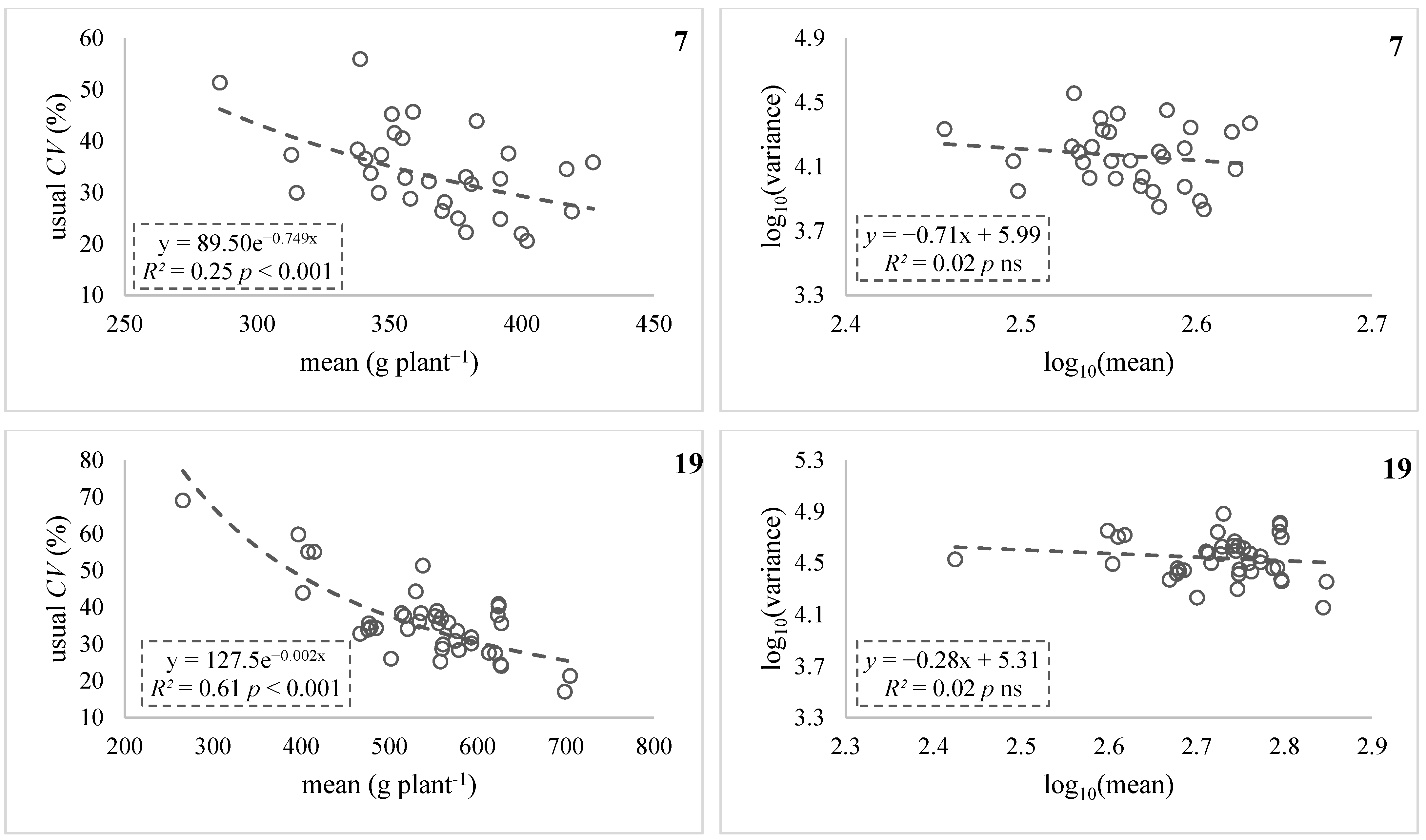
| 7 § | Fasoula [12] | 29 | 286–427 | 21–56 | −0.42 * | −0.14 ns | ||
| Cotton (partial interspecific G. barbadense x G. hirsutum lines) | ||||||||
| 8 | Pankou [27] | 19 | 209–514 | 17–71 | −0.61 ** | +0.29 ns | ||
| 9 | Pankou [27] | 14 | 323–430 | 22–45 | −0.67 ** | −0.42 ns | ||
| Lentil (Lens culinaris L.) | ||||||||
| 10 | Kargiotidou et al. [35] (1st generation) | 19 | 5.75–10.4 | 93–151 | −0.04 ns | |||
| 11 ‡ | Kargiotidou et al. [35] (2nd generation) | 19 | 10.2–27.9 | 84–175 | −0.88 *** | +0.67 *** | +0.62 *** | −0.07 ns |
| 12 | Vlachostergios et al. [36] (Site 1) | 29 | 1.2–6.4 | 30–56 | +0.66 *** | |||
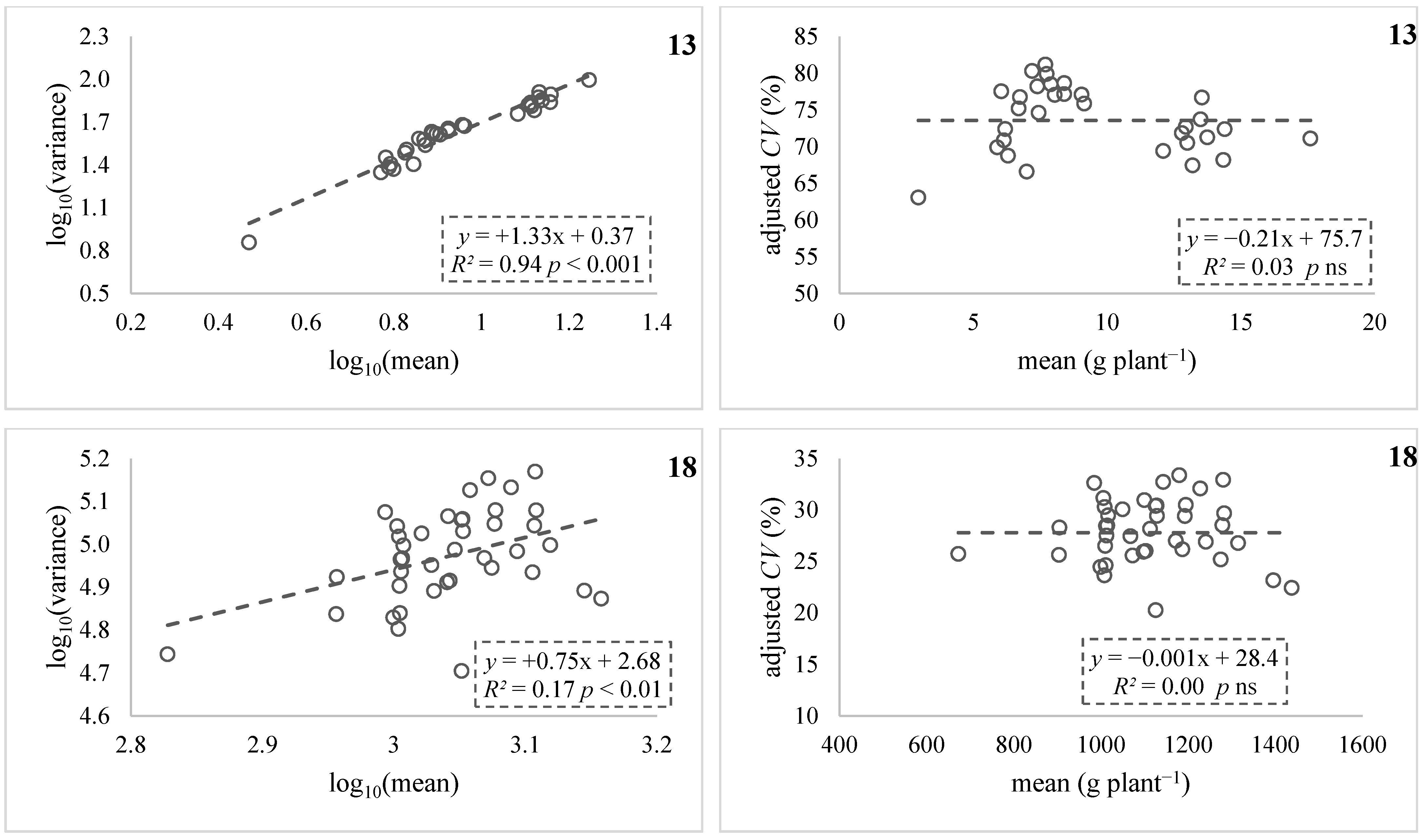
| 13 ‡,§ | Vlachostergios et al. [36] (across 3 sites) | 29 | 2.2–13.7 | 88–163 | −0.81 *** | +0.93 *** | +1.32 *** | −0.10 ns |
| Wheat (Triticum aestivum L.) | ||||||||
| 14 ‡ | Tokatlidis et al. [37] (1st generation) | 19 | 20–34 | 47–75 | −0.82 *** | +0.54 * | +0.64 * | +0.05 ns |
| 15 ‡,§ | Tokatlidis et al. [37] (2nd generation) | 19 | 18–29 | 43–61 | −0.67 *** | +0.68 *** | +1.02 *** | +0.01 ns |
| Maize (Zea mays L.) | ||||||||
| 16 | Tokatlidis et al. [38] (lines A) | 38 | 190–657 | 19–46 | −0.13 ns | |||
| 17 | Tokatlidis et al. [38] (lines B) | 38 | 227–507 | 25–50 | −0.01ns | |||
| 18 ‡ | Tokatlidis et al. [38] (crosses AxB) | 38 | 673–1438 | 19–35 | −0.62 *** | +0.41 ** | +0.75 ** | −0.02 ns |
| 19 § | Greveniotis [28] (HS1) | 39 | 266–699 | 17–69 | −0.77 *** | −0.13 ns | ||
| 20 ‡,§ | Greveniotis [28] (HS2) | 19 | 354–664 | 31–60 | −0.45 * | +0.53 * | +1.13 * | −0.02 ns |
| 21 | Tzantarmas [29] (HS2) | 29 | 418–796 | 30–61 | +0.15 ns | |||
| 22 ‡ | Tzantarmas [29] (HS3) | 19 | 574–1080 | 28–56 | −0.81 *** | +0.49 * | +0.62 * | −0.01 ns |
| 23 § | Tokatlidis et al. (unpublished) (hybrids) | 24 | 625–1169 | 22–41 | −0.76 *** | −0.08 ns | ||
| Soybean (Glycine max (L) Merr.) | ||||||||
| 24 | Fasoula [12] | 19 | 150–212 | 12–23 | −0.24 ns | |||
- Soybean [Glycine max (L) Merr.]
2.2. Data Analysis
2.2.1. Linear Regression of Usual CV against Mean (Stage I)
2.2.2. Testing Variance Dependence on Mean (Stage II)
2.2.3. Conversion of Usual Variance into Adjusted Variance (Stage III)
3. Results
3.1. Linear Regression of Usual CV against Mean (Stage I)
3.2. Testing Variance Dependence on Mean (Stage II)
3.3. Conversion of Usual Variance into Adjusted Variance (Stage III)
4. Discussion
4.1. Soundness of HI
4.1.1. Cases Analyses Confirming the Validity of HI
4.1.2. Case Analyses Not Confirming the Validity of HI
4.2. General Implications
5. Conclusions
Supplementary Materials
Author Contributions
Funding
Data Availability Statement
Conflicts of Interest
Abbreviations
References
- Fasoula, V.A.; Tokatlidis, I.S. Development of crop cultivars by honeycomb breeding. Agron. Sustainable Dev. 2012, 32, 161–180. [Google Scholar] [CrossRef] [Green Version]
- Tokatlidis, I. Crop resilience via inter-plant spacing brings to the fore the productive ideotype. Front. Plant Sci. 2022, 13, 934359. [Google Scholar] [CrossRef] [PubMed]
- Papadakis, J. The relation of the number of tillers per unit area to the yield of wheat and its bearing on fertilizing and breeding this plant-the space factor. Soil Sci. 1940, 50, 369–388. [Google Scholar] [CrossRef]
- Donald, C.M. Competition among crop and pasture plants. Adv. Agron. 1963, 15, 1–118. [Google Scholar] [CrossRef]
- Fasoulas, A.C. (Ed.) The Honeycomb Methodology of Plant Breeding; GR 54006: Thessaloniki, Greece, 1988. [Google Scholar]
- Sedgley, R.H. An appraisal of the Donald ideotype after 21 years. Field Crops Res. 1991, 26, 93–112. [Google Scholar] [CrossRef]
- Fasoulas, A.C. (Ed.) Principles of Crop Breeding; GR 54006: Thessaloniki, Greece, 1993. [Google Scholar]
- Fasoula, D.A.; Fasoula, V.A. Competitive ability and plant breeding. Plant Breed. Rev. 1997, 14, 89–138. [Google Scholar] [CrossRef]
- Tokatlidis, I.S. Crop adaptation to density to optimise grain yield: Breeding implications. Euphytica 2017, 213, 92. [Google Scholar] [CrossRef]
- Fischer, R.A.; Rebetzke, G.J. Indirect selection for potential yield in early-generation, spaced plantings of wheat and other small-grained cereals: A review. Crop Pasture Sci. 2018, 69, 439–459. [Google Scholar] [CrossRef]
- Fasoulas, A. Principles and Methods of Plant Breeding; Department of Genetics and Plant Breeding, Aristolelian University of Thessaloniki: Thessaloniki, Greece, 1981; Volume 11. [Google Scholar]
- Fasoula, V.A. Prognostic breeding: A new paradigm for crop improvement. Plant Breed. Rev. 2013, 37, 297–347. [Google Scholar]
- Fasoulas, A.C.; Zaragotas, D.A. New Developments in the Honeycomb Selection Designs; Pub. 12; Department of Genetics and Plant Breeding, Aristotle University of Thessaloniki: Thessaloniki, Greece, 1990. [Google Scholar]
- Fasoulas, A.C.; Fasoula, V.A. Honeycomb selection designs. Plant Breed. Rev. 1995, 13, 87–139. [Google Scholar] [CrossRef]
- Fasoula, V.A.; Fasoula, D.A. Honeycomb breeding: Principles and applications. Plant Breed. Rev. 2000, 18, 177–250. [Google Scholar]
- Fasoula, V.A.; Fasoula, D.A. Principles underlying genetic improvement for high and stable crop yield potential. Field Crops Res. 2002, 75, 191–209. [Google Scholar] [CrossRef]
- Kargiotidou, A.; Vlachostergios, D.; Tzantarmas, C.; Mylonas, I.; Foti, C.; Menexes, G.; Polidoros, A.; Tokatlidis, I.S. Addressing huge spatial heterogeneity induced by virus infections in lentil breeding trials. J. Biol. Res. Thessalon. 2016, 23, 2. [Google Scholar] [CrossRef] [PubMed] [Green Version]
- Tokatlidis, I.S. Sampling the spatial heterogeneity of the honeycomb model in maize and wheat breeding trials: Analysis of secondary data compared to popular classical designs. Exp. Agric. 2016, 52, 371–390. [Google Scholar] [CrossRef] [Green Version]
- Taylor, S.L.; Payton, M.E.; Raun, W.R. Relationships between mean yield, coefficient of variation, mean square error, and plot size in wheat field experiments. Commun. Soil Sci. Plant Anal. 1999, 30, 1439–1447. [Google Scholar] [CrossRef]
- Döring, T.F.; Knapp, S.; Cohen, J.E. Taylor’s power law and the stability of crop yields. Field Crops Res. 2015, 183, 294–302. [Google Scholar] [CrossRef]
- Döring, T.F.; Reckling, M. Detecting global trends of cereal yield stability by adjusting the coefficient of variation. Eur. J. Agron. 2018, 99, 30–36. [Google Scholar] [CrossRef]
- Knapp, S.; van der Heijden, M.G.A. A global meta-analysis of yield stability in organic and conventional agriculture. Nat. Commun. 2018, 9, 3632. [Google Scholar] [CrossRef] [Green Version]
- Reckling, M.; Döring, T.F.; Bergkvist, G.; Stoddard, F.L.; Watson, C.A.; Seddi, S.; Chmielewski, F.-M.; Bachinger, J. Grain legume yields are as stable as other spring crops in long-term experiments across northern Europe. Agron. Sustainable Dev. 2018, 38, 63. [Google Scholar] [CrossRef] [Green Version]
- Smutná, P.; Tokatlidis, I.S. Testing Taylor’s Power Law association of winter wheat variation with mean yield at two contrasting soils. Eur. J. Agron. 2021, 126, 126268. [Google Scholar] [CrossRef]
- Tokatlidis, I.S.; Remountakis, E. The Impacts of interplant variation on aboveground biomass, grain yield, and harvest index in maize. Int. J. Plant Prod. 2020, 14, 57–65. [Google Scholar] [CrossRef]
- Pankou, C.; Koulymboudi, L.; Papathanasiou, F.; Gekas, F.; Papadopoulos, I.; Sinapidou, E.; Tokatlidis, I.S. Testing Taylor’s Power Law association of maize interplant variation with mean grain yield. J. Integr. Agric. 2022, 21, 3569–3577. [Google Scholar] [CrossRef]
- Pankou, C. Effect of Reciprocal crosses on the Stability of Partial Interspecific Lines and Improvement of Cotton Varieties. Ph.D. Thesis, Aristotle University of Thessaloniki/School of Agriculture, Thessaloniki, Greece, 2015. (In Greek with Abstract in English). [Google Scholar]
- Greveniotis, V. Investigating the Possibility of Replacing Maize Hybrids with Open Pollinated Lines. Ph.D. Thesis, Democritus University of Thrace/Department of Agricultural Development, Orestiada, Greece, 2012. (In Greek with Abstract in English). [Google Scholar]
- Tzantarmas, C. Investigating the Possibility of Recombination of Favorable Genes from Different Maize Hybrids to Develop Improved Open Pollinated Lines. Ph.D. Thesis, Democritus University of Thrace/Department of Agricultural Development, Orestiada, Greece, 2016. (In Greek with Abstract in English). [Google Scholar]
- Papathanasiou, F.; Papadopoulou, F.; Mylonas, I.; Ninou, E.; Papadopoulos, I. Single-plant selection at ultra-low density of first generation lines of three been cultivars under water stress. Agric. For. 2019, 65, 27–34. [Google Scholar] [CrossRef]
- Tokatlidis, I.S.; Papadopoulos, I.I.; Baxevanos, D.; Koutita, O. Genotype × Environment effects on single-plant selection at low density for yield and stability in climbing dry bean. Crop Sci. 2010, 50, 775–783. [Google Scholar] [CrossRef]
- Tokatlidis, I.S.; Tsikrikoni, C.; Tsialtas, J.T.; Lithourgidis, A.S.; Bebeli, P. Variability within cotton cultivars for yield, fibre quality and physiological traits. J. Agric. Sci. 2008, 146, 483–490. [Google Scholar] [CrossRef]
- Mavromatis, A.G.; Kadarzi, S.K.; Vlachostergios, D.N.; Xynias, I.N.; Skaracis, G.N.; Roupakias, D.G. Induction of embryo development and fixation of partial interspecific lines after pollination of F1 cotton interspecific hybrids (Gossypium barbadense x Gossypium hirsutum) with pollen from Hibiscus cannabinus. Aust. J. Agric. Res. 2005, 56, 1101–1109. [Google Scholar] [CrossRef]
- Kargiotidou, A. Pedigree and Mass Selection for Yield in a Lentil Population under Low-Density, Low-Input Conditions, and the Influence of Selection Intensity on Grain Productivity and Tolerance to Viruses. Ph.D. Thesis, Democritus University of Thrace/Department of Agricultural Development, Orestiada, Greece, 2012. (In Greek with abstract in English). [Google Scholar]
- Kargiotidou, A.; Chatzivassiliou, E.; Sinapidou, E.; Papageorgiou, A.; Skaracis, G.; Tokatlidis, I.S. Selection at ultra-low density highlights plants escaping virus infection and leads towards high-performing pure-line cultivars in lentil. J. Agric. Sci. 2014, 152, 749–758. [Google Scholar] [CrossRef]
- Vlachostergios, D.N.; Tzantarmas, C.; Kargiotidou, A.; Ninou, E.; Pankou, C.; Gaintatzi, C.; Mylonas, I.; Papadopoulos, I.; Foti, C.; Chatzivassiliou, E.; et al. Single-plant selection within lentil landraces at ultra-low density: A short-time tool to breed high yielding and stable varieties across divergent environments. Euphytica 2018, 214, 58. [Google Scholar] [CrossRef]
- Tokatlidis, I.S.; Xynias, I.N.; Tsialtas, J.T.; Papadopoulos, I.I. Single-plant selection at ultra-low density to improve stability of a bread wheat cultivar. Crop Sci. 2006, 46, 90–97. [Google Scholar] [CrossRef]
- Tokatlidis, I.S.; Koutsika-Sotiriou, M.; Fasoulas, A.C.; Tsaftaris, A.S. Improving maize hybrids for potential yield per plant. Maydica 1998, 43, 123–129. [Google Scholar]
- Greveniotis, V.; Fasoula, V.A.; Papadopoulos, I.I.; Sinapidou, E.; Tokatlidis, I.S. Bridging the productivity gap between maize inbreds and hybrids via selection of plants excelling in crop yield genetic potential. Aust. J. Crop Sci. 2012, 6, 1448–1454. [Google Scholar]
- Nielsen, D.C.; Vigil, M.F. Wheat yield and yield stability of eight dryland crop rotations. Agron. J. 2018, 110, 594–601. [Google Scholar] [CrossRef] [Green Version]
- Andrade, F.H.; Abbate, P.E. Response of maize and soybean to variability in stand uniformity. Agron. J. 2005, 97, 1263–1269. [Google Scholar] [CrossRef] [Green Version]
- Fasoula, V.A.; Tollenaar, M. The impact of plant population density on crop yield and response to selection in maize. Maydica 2005, 50, 9–48. [Google Scholar]
- Taylor, R.A.J.; Lindquist, R.K.; Shipp, J.L. Variation and consistency in spatial distribution as measured by Taylor’s power law. Environ. Entomol. 1998, 27, 191–201. [Google Scholar] [CrossRef]
- Pan, X.Y.; Wang, G.X.; Yang, H.M.; Wei, X.P. Effect of water deficits on within-plot variability in growth and grain yield of spring wheat in northwest China. Field Crops Res. 2003, 80, 195–205. [Google Scholar] [CrossRef]
- Kargiotidou, A.; Tzantarmas, C.; Chatzivassiliou, E.; Tokatlidis, I.S. Seed propagation at low density facilitates the selection of healthy plants to produce seeds with a reduced virus load in a lentil landrace. Seed Sci. Technol. 2015, 43, 31–39. [Google Scholar] [CrossRef]
- Vlachostergios, D.N.; Roupakias, D.G. Screening under low-plant density reinforces the identification of lentil plants with resistance to fusarium wilt. Crop Sci. 2017, 57, 1285–1294. [Google Scholar] [CrossRef]


| S5 × S5 | μ (g Plant−1) | S5 × S5 | CV | HI | S5 × S5 | ||
|---|---|---|---|---|---|---|---|
| A29 × B3 | 1438 | A29 × B3 | 0.19 | 5.26 | A2 × B26 | 0.20 | 4.94 |
| A16 × B31 | 1396 | A16 × B31 | 0.20 | 5.00 | A29 × B3 | 0.22 | 4.46 |
| A22 × B23 | 1315 | A2 × B26 | 0.20 | 5.00 | A16 × B31 | 0.23 | 4.32 |
| A32 × B4 | 1283 | A36 × B11 | 0.23 | 4.35 | A9 × B2 | 0.24 | 4.23 |
| A14 × B39 | 1281 | A22 × B23 | 0.24 | 4.17 | A37 × B33 | 0.24 | 4.09 |
| A10 × B18 | 1279 | A40 × B24 | 0.25 | 4.00 | A1 × B6 | 0.25 | 4.06 |
| A36 × B11 | 1275 | A28 × B14 | 0.25 | 4.00 | A36 × B11 | 0.25 | 3.97 |
| A40 × B24 | 1241 | A9 × B2 | 0.25 | 4.00 | A26 × B27 | 0.26 | 3.91 |
| A30 × B30 | 1228 | A10 × B18 | 0.26 | 3.85 | A38 × B36 | 0.26 | 3.90 |
| A15 × B35 | 1195 | A25 × B12 | 0.26 | 3.85 | A12 × B9 | 0.26 | 3.89 |
| A8 × B16 | 1193 | A31 × B17 | 0.26 | 3.85 | A18 × B40 | 0.26 | 3.86 |
| A28 × B14 | 1187 | A18 × B40 | 0.26 | 3.85 | A31 × B17 | 0.26 | 3.85 |
| A17 × B5 | 1180 | A26 × B27 | 0.26 | 3.85 | A28 × B14 | 0.26 | 3.82 |
| A25 × B12 | 1172 | A1 × B6 | 0.26 | 3.85 | A3 × B29 | 0.27 | 3.77 |
| A39 × B1 | 1143 | A37 × B33 | 0.26 | 3.85 | A22 × B23 | 0.27 | 3.73 |
| A5 × B22 | 1129 | A32 × B4 | 0.27 | 3.70 | A40 × B24 | 0.27 | 3.72 |
| A7 × B34 | 1128 | A8 × B16 | 0.28 | 3.57 | A25 × B12 | 0.27 | 3.70 |
| A2 × B26 | 1126 | A21 × B20 | 0.28 | 3.57 | A6 × B10 | 0.27 | 3.64 |
| A24 × B8 | 1126 | A6 × B10 | 0.28 | 3.57 | A11 × B28 | 0.28 | 3.64 |
| A21 × B20 | 1113 | A3 × B29 | 0.28 | 3.57 | A21 × B20 | 0.28 | 3.55 |
| A31 × B17 | 1103 | A15 × B35 | 0.29 | 3.45 | A34 × B19 | 0.28 | 3.53 |
| A35 × B15 | 1100 | A5 × B22 | 0.29 | 3.45 | A19 × B38 | 0.28 | 3.52 |
| A18 × B40 | 1098 | A11 × B28 | 0.29 | 3.45 | A23 × B37 | 0.28 | 3.51 |
| A26 × B27 | 1073 | A38 × B36 | 0.29 | 3.45 | A10 × B18 | 0.29 | 3.51 |
| A6 × B10 | 1068 | A14 × B39 | 0.30 | 3.33 | A8 × B16 | 0.29 | 3.40 |
| A33 × B13 | 1050 | A30 × B30 | 0.30 | 3.33 | A5 × B22 | 0.29 | 3.40 |
| A4 × B21 | 1017 | A7 × B34 | 0.30 | 3.33 | A4 × B21 | 0.29 | 3.39 |
| A23 × B37 | 1015 | A24 × B8 | 0.30 | 3.33 | A32 × B4 | 0.30 | 3.37 |
| A11 × B28 | 1013 | A23 × B37 | 0.30 | 3.33 | A33 × B13 | 0.30 | 3.33 |
| A19 × B38 | 1012 | A19 × B38 | 0.30 | 3.33 | A13 × B32 | 0.30 | 3.30 |
| A1 × B6 | 1011 | A35 × B15 | 0.31 | 3.23 | A24 × B8 | 0.30 | 3.29 |
| A3 × B29 | 1010 | A33 × B13 | 0.31 | 3.23 | A7 × B34 | 0.30 | 3.29 |
| A13 × B32 | 1009 | A4 × B21 | 0.31 | 3.23 | A15 × B35 | 0.30 | 3.28 |
| A9 × B2 | 1008 | A17 × B5 | 0.32 | 3.13 | A35 × B15 | 0.31 | 3.23 |
| A27 × B7 | 1006 | A39 × B1 | 0.32 | 3.13 | A27 × B7 | 0.31 | 3.21 |
| A37 × B33 | 999 | A13 × B32 | 0.32 | 3.13 | A30 × B30 | 0.32 | 3.12 |
| A20 × B25 | 985 | A34 × B19 | 0.32 | 3.13 | A20 × B25 | 0.33 | 3.07 |
| A34 × B19 | 905 | A27 × B7 | 0.33 | 3.03 | A39 × B1 | 0.33 | 3.06 |
| A38 × B36 | 904 | A20 × B25 | 0.35 | 2.86 | A14 × B39 | 0.33 | 3.04 |
| A12 × B9 | 673 | A12 × B9 | 0.35 | 2.86 | A17 × B5 | 0.33 | 3.00 |
Disclaimer/Publisher’s Note: The statements, opinions and data contained in all publications are solely those of the individual author(s) and contributor(s) and not of MDPI and/or the editor(s). MDPI and/or the editor(s) disclaim responsibility for any injury to people or property resulting from any ideas, methods, instructions or products referred to in the content. |
© 2023 by the authors. Licensee MDPI, Basel, Switzerland. This article is an open access article distributed under the terms and conditions of the Creative Commons Attribution (CC BY) license (https://creativecommons.org/licenses/by/4.0/).
Share and Cite
Tokatlidis, I.S.; Vrochidis, I.; Sistanis, I.; Pankou, C.I.; Sinapidou, E.; Papathanasiou, F.; Vlachostergios, D.N. Testing the Validity of CV for Single-Plant Yield in the Absence of Competition as a Homeostasis Index. Agronomy 2023, 13, 176. https://doi.org/10.3390/agronomy13010176
Tokatlidis IS, Vrochidis I, Sistanis I, Pankou CI, Sinapidou E, Papathanasiou F, Vlachostergios DN. Testing the Validity of CV for Single-Plant Yield in the Absence of Competition as a Homeostasis Index. Agronomy. 2023; 13(1):176. https://doi.org/10.3390/agronomy13010176
Chicago/Turabian StyleTokatlidis, Ioannis S., Iordanis Vrochidis, Iosif Sistanis, Chrysanthi I. Pankou, Evaggelia Sinapidou, Fokion Papathanasiou, and Dimitrios N. Vlachostergios. 2023. "Testing the Validity of CV for Single-Plant Yield in the Absence of Competition as a Homeostasis Index" Agronomy 13, no. 1: 176. https://doi.org/10.3390/agronomy13010176