Adaptability Evaluation of the Spatiotemporal Fusion Model in the Summer Maize Planting Area of the Southeast Loess Plateau

Abstract

Precise regional crop yield estimates based on the high-spatiotemporal-resolution remote sensing data are essential for directing agronomic practices and policies to increase food security. This study used the enhanced spatial and temporal adaptive reflectance fusion model (ESTARFM), the flexible spatiotemporal data fusion (FSADF), and the spatial and temporal non-local filter based fusion model (STNLFFM) to calculate the normalized differential vegetation index (NDVI) of the summer maize planting area in the Southeast Loess Plateau based on the Sentinel-2 and MODIS data. The spatiotemporal resolution was 10 m and 1 d, respectively. Then, we evaluated the adaptability of the ESTARFM, FSADF, and STNLFFM fusion models in the field from the perspectives of spatial and textural characteristics of the data, summer maize NDVI growing curves, and yield estimation accuracy through qualitative visual discrimination and quantitative statistical analysis. The results showed that the fusion of ESTARFM–NDVI, FSDAF–NDVI, and STNLFFM–NDVI could precisely represent the variation tendency and local mutation information of NDVI during the growth period of summer maize, compared with MODIS–NDVI. The correlation between STNLFFM–NDVI and Sentinel-2–NDVI was favorable, with large correlation coefficients and a small root mean square error (RMSE). In the NDVI growing curve simulation of summer maize, STNLFFM introduced overall weights based on non-local mean filtering, which could significantly improve the poor fusion results at seedling and maturity stages caused by the long gap period of the high-resolution data in ESTARFM. Moreover, the accuracy of yield estimation was as follows (from high to low): STNLFFM (R = 0.742, mean absolute percentage error (MAPE) = 6.22%), ESTARFM (R = 0.703, MAPE = 6.80%), and FSDAF (R = 0.644, MAPE = 10.52%). The FADSF fusion model was affected by the spatial heterogeneity in the semi-humid areas, and the yield simulation accuracy was low. In the semi-arid areas, the FADSF fusion model had the advantages of less input data and a faster response.

1. Introduction

Currently, remote sensing has become the dominant method for crop yield estimation [1,2]. The traditional methods of crop yield estimation generally adopt a sampling survey and field observation approach, which is not suitable for crop yield estimation in large areas [3,4]. Remote sensing yield estimation can macroscopically and dynamically monitor in real time, and provide more scientific monitoring methods for crop growth and yield prediction [5]. In crop yield estimation research, net primary production (NPP) of vegetation plays an important role [6,7]. NPP is the amount of organic matter fixed with green plants per unit area and per unit time, and is the fraction of organic carbon fixed with photosynthesis minus the fraction consumed with plant respiration, which has a direct impact on crop yield [8]. Existing models for estimating NPP are generally divided into four categories: the climate productivity model [9], physiological and ecological process model [10], light use efficiency model [11], and ecological remote sensing coupling model [12]. Among them, the climate productivity model and physiological and ecological process model have complex mechanisms, require many parameters, and have large errors in regional scale simulation results [13]. Moreover, human factors have a great influence on parameter determination of the ecological remote sensing coupling model [14]. The light use efficiency model characterized by the Carnegie–Ames–Stanford Approach (CASA), with its few input parameters and strong operability, is widely used in the process of regional scale NPP estimation [11,15]. CASA, which can forecast crop yield at various scales, has the largest concordance with MODIS–NPP and observed values when compared to the statistical model and process model [16]. Since the majority of the parameters required for it can be obtained from remote sensing sources, the problem of the insufficient ground station data has been essentially eliminated [17]. Former research have shown that the normalized differential vegetation index (NDVI) has a great influence on the simulation accuracy of NPP, as the basic data input to the CASA model [18]. The multitemporal NDVI data with high spatial resolution can achieve accurate NPP inversion, NPP dynamic monitoring on continuous time scales, and vegetation or crop growth analysis, in order to improve yield estimation accuracy [19]. Therefore, accurate yield estimation using remote sensing images with a high time/space resolution is a key content for developing high-yield, high-quality, ecological and safe agriculture in the area.

Due to the rapidly changing crops during the growing season, the period-specific multiple temporal sequence data and high-spatial-resolution NDVI data are needed to ensure the simulation accuracy, but the available remote sensing data are deficient in either temporal or spatial resolution [20]. The spatiotemporal fineness of the remote sensing data has become an important factor restricting its application in agriculture. NDVI with high spatial resolution can obtain rich crop details at a regional scale; however, due to the long revisit cycle, the critical period of crop growth cannot meet the requirements of dynamic tracking and monitoring. NDVI with high time resolution revisits at short intervals, but its spatial resolution is low. The problem of mixed pixels is more prominent, which causes the problem of inaccurate simulated crop information. The spatiotemporal fusion method of multiple remote sensing sources may concurrently obtain the spatial texture information of the high-spatial-resolution data and the temporal phase information of the high-temporal-resolution data, which has become a key technical means to simulate NDVI during the crop growth period [21]. For the purpose of creating a sequence of “temporally dense” images of high spatial resolution, spatiotemporal fusion of images fuses a “temporally dense” image of low spatial resolution with a “temporally sparse” image of high spatial resolution that corresponds to a point in time [22]. The three categories of current spatiotemporal fusion models are approximately as follows. The first method is transformation-based, which transforms the data before processing it. Wavelet transformation is employed to depict its inverse transformation in order to produce a high-resolution image at the time of prediction. Although this mechanism has the advantage of retaining comprehensive spectral information, it also has the disadvantage of pixel mixing and low fusion accuracy [23,24]. The second approach involves a machine learning-based spatiotemporal fusion model that leverages sparse representations for image processing. Using a two-layer spatiotemporal fusion model, which captures the varying surface reflectance in the photographs, these models consider variations in the resolution of the data. Nevertheless, the high data requirements and their inefficiency make them inappropriate for large-scale research [25,26]. In the fusion model based on reconstruction, it is postulated that the reflectance of low-spatial-resolution pixels can be expressed as a linear combination of the reflectance values from high-spatial-resolution pixels. This represents the third model in our study. These models consider non-linear reflectance change characteristics as well as geographical heterogeneity. The algorithm, which is extensively used, has significantly increased fusion accuracy while keeping more spatial features in areas with high heterogeneity [27,28]. Typical models include the spatial and temporal adaptive reflectance fusion model (STARFM) [29], the enhanced spatial and temporal adaptive reflectance fusion model (ESTARFM) [30], the flexible spatiotemporal data fusion (FSADF) [31], and the spatial and temporal non-local filter-based fusion model (STNLFFM) [32]. STARFM was proposed earlier. It effectively realized the spatiotemporal fusion of the Landsat and MODIS image data. It has a high accuracy for large homogeneous areas, but poor applicability for areas with strong instantaneous changes and fractured topography [33]. By fully accounting for pixel heterogeneity, ESTARFM improves the procedure for calculating spectral weighting factors within the STARFM model. In order to improve the model’s reflectance fusion accuracy in regions of high heterogeneity, the ESTARFM model adds the conversion coefficients for pure and mixed pixel reflectance changes. This is extremely useful in large-area remote sensing applications, and its fusion works well in general [30,33]. Similarly, founded on the STARFM framework, the FSDAF model improves the accessibility of high-resolution time-series data and reduces the number of data sources by means of a fast surface detection method. Only two low-resolution images and one high-resolution image are required as inputs, and the model has a fast response speed [31,33]. Based on weight function of non-local mean filtering, the relationship between reference and target time–phase images of the STNLFFM model was calculated with non-local similar pixels, which effectively improved the fusion accuracy and was widely used [32,33]. Many studies have compared and analyzed different spatiotemporal data fusion models from fusion accuracy and regional adaptability. Hobyb et al. [34] used STARFM, ESTARFM, and FSDAF models to integrate the Landsat 8 and MODIS data to generate the high-spatiotemporal-resolution NDVI data in an arid region of Tadla, and the results showed that the ESTARFM algorithm had the best effect and could effectively reduce the error. Lei et al. [33] comprehensively evaluated the fusion effect of STARFM, ESTARFM, FSDAF, and STNLFFM from multiple perspectives based on “Point–Line –Plane”, and found that FSDAF was greatly affected with window size in predicting complex ground object images, and found that the STNLFFM fusion algorithm was generally superior to the other three fusion algorithms. Fan et al. [35] evaluated the applicability of the STARFM, ESTARFM, and FSADF fusion methods in a typical area of the Three-River Headwater Region. They found that the STARFM and FSADF models had better fusion effect and higher accuracy, and optimum window of the model was 50. Most studies focus on the evaluation of fusion results of the MODIS and Landsat data, and there is a lack of studies on the fusion of the Sentinel 2 and MODIS data [33,36]. The Sentinel-2 data with high spatial resolution and strong stability are being widely employed as remote sensing technology advances. The choice of the fusion model for the Sentinel-2 data has emerged as an issue to be investigated. Additionally, as satellite images with high spatial resolution get wider, the data processing complexity rises as well. It is also important to investigate how well the conventional spatiotemporal fusion model adapts to two data sources with significant size variations.

The Loess Plateau is a typical arid and semi-arid continental monsoon climate zone with a long history of watershed agriculture and valley reclamation, which plays an essential role in guaranteeing national food security and grain production [37]. The Yuncheng Basin is an important grain producing area in the southeast of the Loess Plateau, but it has a large degree of topographic fragmentation [11]. Due to the limited spatial resolution of the MODIS–NDVI data (500 m), it is challenging to distinguish the finer features of the spatial textures of different surface objects. Additionally, mixed pixels are the main cause of NDVI curve lag. The spatiotemporal fusion model can combine the high-resolution data at the corresponding time, solve the problem of MODIS data mixing pixels, and effectively adjust the inaccurate information of NDVI changes. At the same time, it can solve the discretization problem of the high-resolution data on time series, and better reflect the spatial details and textures of summer maize on continuous time scale. Accurate monitoring of crop growth and estimation of yield using the NDVI data with high time and space resolution is the key to agricultural development in this region. This study evaluated the adaptability of ESTARFM, FSADF, and STNLFFM fusion models in the Yuncheng Basin with qualitative visual discrimination and quantitative statistical analysis, and determined the best NDVI fusion model in this area, which provided the NDVI data with high accuracy for summer maize yield estimation and improved yield estimation accuracy.

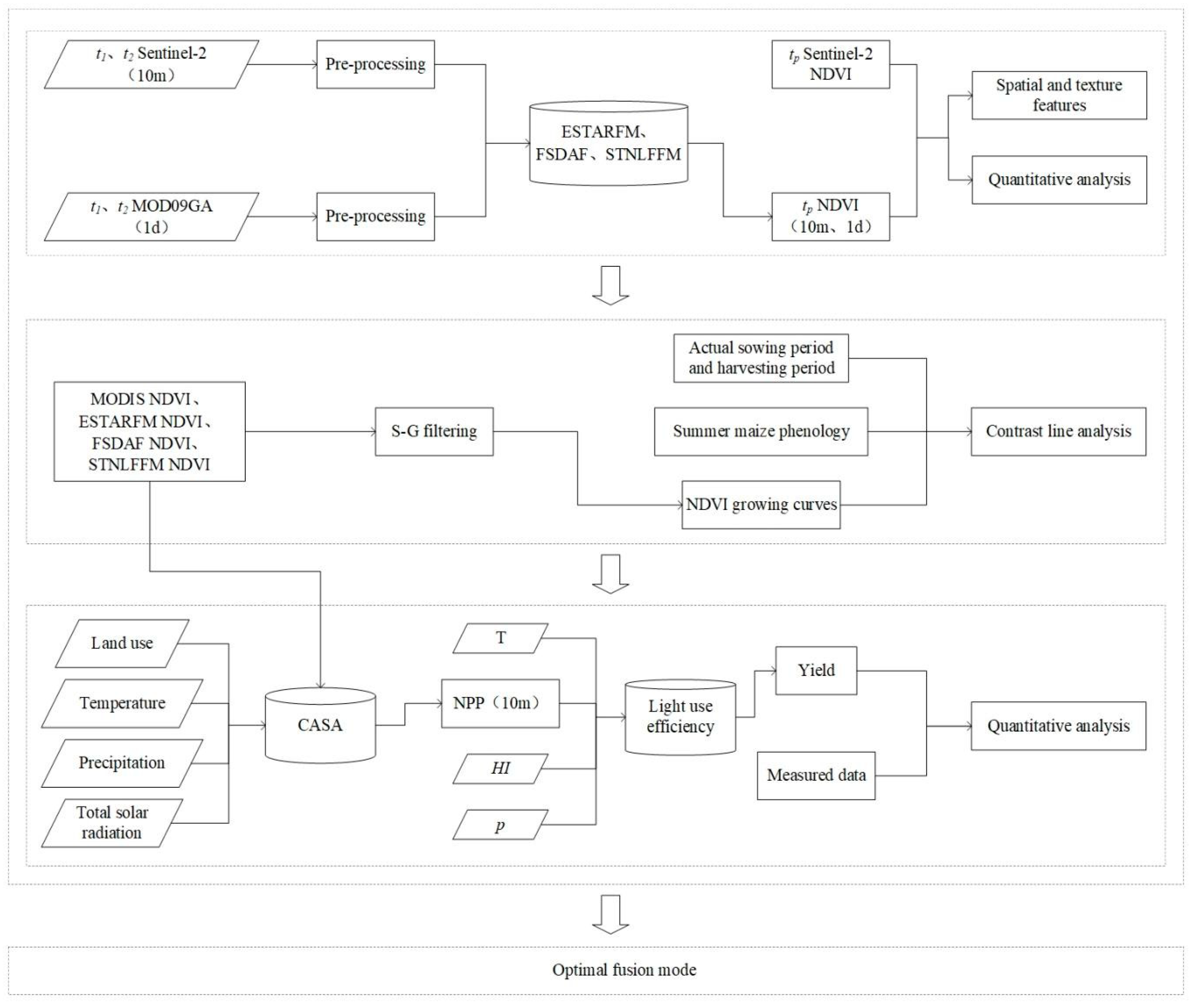
2. Materials and Methods

2.1. Study Area

The Yuncheng Basin is located in the semi-humid and semi-arid region (34°40′–35°38′ N, 110°15′–111°46′ E) in the Southeast Loess Plateau. It is bounded to the north by the Zijin Mountain-Emei Terraces and to the southeast by the Zhongtiao Mountains. It faces the Guanzhong Plain across the Yellow River to the west as well as seven county-level administrative areas from east to west, including Jiangxian County, Wenxi County, Xia County, Yanhu District, Wanrong County, Linyi County, and Yongji City (Figure 1). The average monthly temperatures in the Yuncheng Basin range from 5 to 24 °C, precipitation reaches a maximum of 178 mm in August, and total monthly solar radiation ranges from 434 to 847 MJ/m². The area exhibits a zonal climatic pattern with noticeable variations in altitude, making it conducive for cultivating crops such as wheat and corn [38]. Moreover, it serves as a significant hub for grain production in the northern region of China. Moreover, this area is also a typical hilly area of the Loess Plateau. The terrain fragmentation and the lack of water resources are the main factors limiting the development of agriculture in this area [11].

2.2. Data Sources

On the dates listed below in 2020, Sentinel-2A and Sentinel-2B in splice domains T49SDU, T49SDV, T49SEU, and T49SEV were downloaded from the European Space Agency (https://scihub.copernicus.eu/dhus/#/home, accessed on 1 May 2022); the dates are, respectively, 5 April, 24 June, 2 September, 22 October, 10 February, 10 May, 28 August, and 6 November. To calculate the NDVI with a spatial resolution of 10 m, Sentinel Application Platform (SNAP) software (9.0) was used to resample, stitch, and convert the projection. NASA (https://ladsweb.modaps.eosdis.nasa.gov/, accessed on 25 June 2022) provided the H26V05 and H27V05 orbital MODIS reflectance products MOD09GA with a spatial resolution of 500 m and a temporal resolution of 1 day. Based on the stitching of the images and the conversion of the MOD09GA to UTM projection, the NDVI (500 m, 1 d) was calculated by the R band and NIR band.

The monthly temperature and precipitation information from 23 meteorological stations near the study area were made available on the China Meteorological Administration website (http://data.cma.cn/, accessed on 23 December 2022). The monthly solar radiation was also considered, and it was calculated using the Angstrom–Prescott method using the daily sunshine hours observed. The topographical data for the research region using the ASTER GDEM 30 m product was obtained via the “Geospatial Data Cloud Platform” (http://www.gscloud.cn, accessed on 27 December 2022). Using the interpolation tool (ANUSPLIN), the spatially interpolated meteorological data for the region were gathered. Latitude and longitude served as the independent variables, and elevation served as the covariate.

The sowing and harvesting dates, irrigation levels, yield, stem and leaf yield, etc. were all included in the data for the summer maize sample points. The sampling area was 3 by 3 m, and a portable GPS was used to record the center location of sample area (Figure 1). The yield per unit area was estimated after five uniformly distributed sites in the sample area were sampled, dried, and weighed. Using the average yield per unit area of the five sample locations, the measured yield of summer maize in the sample area was computed.

2.3. Analysis Methodology

2.3.1. ESTARFM Model

The ESTARFM model presupposes the correlation and stability of the systematic deviation among the remote sensing data from different sources collected over a specific time period [30]. It uses the following formula:

$$NDV{I}_k(X_{\omega /2},Y_{\omega /2},t_p)=NDV{I}_O(X_{\omega /2},Y_{\omega /2},t_k)+{\displaystyle \sum _{\mathrm{i}=1}^N{W}_i{V}_i\left[M(X_i,Y_i,t_p)-M(X_i,Y_i,t_k)\right]}$$

(1)

where NDVI_k is a high-resolution-predicted NDVI at time k; NDVI_O is the Sentinel-2–NDVI at time k; M represents the MODIS–NDVI for the corresponding period; ω is the sliding window’s size; (X_ω/2, Y_ω/2) represents the sliding window center pixel location; N is the number of similarity pixels in the sliding window; (X_i, Y_i) is the location of similarity pixel i; V_i represents the conversion coefficient, which is the regression coefficient of the two groups of high-resolution and low-resolution NDVI on the corresponding date; and W_i represents the weights of similarity pixels i. The forecast NDVI at m and n times were then utilized to compute the final forecast NDVI. The calculation formula is as follows:

$$NDVI(X_{\omega /2},Y_{\omega /2},t_p)=T_m\times NDV{I}_m(X_{\omega /2},Y_{\omega /2},t_p)+T_n\times NDV{I}_n(X_{\omega /2},Y_{\omega /2},t_p)$$

(2)

where NDVI is the NDVI of the final prediction date; NDVI_m is the predicted NDVI at time m; NDVI_n is the predicted NDVI at time n; T_m and T_n are the weight factors at times m and n.

$$T_k=\frac{1/\left|{\displaystyle {\sum }_{j=1}^{\omega }{\displaystyle {\sum }_{i=1}^{\omega }M\left(X_i,Y_i,t_k\right)}}-{\displaystyle {\sum }_{j=1}^{\omega }{\displaystyle {\sum }_{i=1}^{\omega }M\left(X_i,Y_i,t_p\right)}}\right|}{\left(1/\left|{\displaystyle {\sum }_{j=1}^{\omega }{\displaystyle {\sum }_{i=1}^{\omega }M\left(X_i,Y_i,t_k\right)}}-{\displaystyle {\sum }_{j=1}^{\omega }{\displaystyle {\sum }_{i=1}^{\omega }M\left(X_i,Y_i,t_p\right)}}\right|\right)}$$

(3)

2.3.2. FSDAF Model

A pair of low-spatial-resolution images taken at times t₀ and t₁, as well as a high-spatial-resolution image taken at time t₀, make up the input data for the FSDAF model [31]. The model uses the following formula:

$$R_{high1}(x_{ij},y_{ij},b)=R_{high0}(x_{ij},y_{ij},b)+{\displaystyle \sum _{k=1}^n{w}_k\times \mathsf{\Delta }R(x_k,y_k,b)}$$

(4)

where R_high1(x_ij,y_ij,b) is the high-resolution NDVI of the t₁ moment to be predicted; R_high0(x_ij,y_ij,b) is high-resolution NDVI at t₀; w_k is the weight of the KTH similar pixel; and its calculation method is consistent with the ESTARFM model. ∆R(x_k,y_k,b) is the change in pixel resolution between time t₀ and time t₁, calculated as follows:

$$\mathsf{\Delta }R(x_{ij},y_{ij},b)=\epsilon (x_{ij},y_{ij},b)+\mathsf{\Delta }R(a,b)$$

(5)

where ∆R(a,b) is the change of category a in high-resolution NDVI between time t₀ and time t₁; ɛ(x_ij,y_ij,b) is the residual error from the i low-resolution pixel to the j high-resolution pixel, calculated as follows:

$$\epsilon (x_{ij},y_{ij},b)=m\times L(x_j,y_j,b)\times W(x_{ij},y_{ij},b)$$

(6)

where m is the number of sub-pixels in a low-resolution pixel; W(x_ij,y_ij,b) is the weight after normalization of LW(x_ij,y_ij,b); L(x_j,y_j,b) is the residual of high-resolution real NDVI and model-predicted NDVI, calculated as follows:

$$LW(x_{ij},y_{ij},b)=E_{ho}(x_{ij},y_{ij},b)+\epsilon (x_j,y_j,b)\times \left[1-HI(x_{ij},y_{ij})\right]$$

(7)

$$E_{ho}(x_{ij},y_{ij},b)=R_{high1}{}^{SP}(x_{ij},y_{ij},b)-R_{high1}{}^{TP}(x_{ij},y_{ij},b)$$

(8)

$$L(x_j,y_j,b)=\mathsf{\Delta }L(x_j,y_j,b)-\frac{1}{m}\times [{\displaystyle \sum _{j=1}^m{R}_{high1}{}^{TP}(x_{ij},y_{ij},b)}-{\displaystyle \sum _{j=1}^m{R}_{high0}(x_{ij},y_{ij},b)}]$$

(9)

where R_high1^TP(x_ij,y_ij,b) is the high-resolution NDVI pixel value of t₁ moment predicted with time difference; R_high1^SP(x_ij,y_ij,b) is the NDVI pixel value predicted after optimizing the parameters of the thin-plate spline interpolation function; and H(x_ij,y_ij) is the coefficient of homogeneity.

2.3.3. STNLFFM Model

STNLFFM is a spatiotemporal model that enhances fusion accuracy by improving the weighting function and conversion relationship between the high-resolution data [32]. Its calculation formula is as follows:

$$F(x,y,t_p)={\displaystyle \sum _{k=1}^M{\displaystyle \sum _{i=1}^{N}W(x_i,y_i,t_k)}}\times \left[a(x_i,y_i,\mathsf{\Delta }{t}_k)\times F(x_i,y_i,t_k)+b(x_i,y_i,\mathsf{\Delta }{t}_k)\right]$$

(10)

where F(x,y,t_p) is the Sentinel-2–NDVI of a target pixel (x,y) at prediction date t_p; M is the reference date’s number; N is the number of similar pixels (pixels of the same type as the target pixel) in the images; (x_i,y_i) is the location of the ith similar pixel; a(x_i,y_i,Δt_k); and b(x_i,y_i,Δt_k) are linear fitting coefficients of the set of similar pixels in low-spatial-resolution images between reference moment t_k and prediction moment t_p, respectively, where the latter two are calculated using the least squares method. W(x_i,y_i,t_k) is the weight of the ith comparable pixel of the Sentinel-2–NDVI at the reference instant t_k in the following formula:

$$W(x_i,y_i,t_k)=W_{individual}(x_i,y_i,t_k)\times W_{whole}(x_i,y_i,t_k)$$

(11)

$$W_{individual}(x_i,y_i,t_k)=\exp \left(-\frac{G\times \Vert C(x_i,y_i,t_k)-C(x_i,y_i,t_p)\Vert }{h^2}\right)$$

(12)

$$W_{whole}(x_i,y_i,t_k)=\frac{1/{\displaystyle {\sum }_{i=1}^{\omega }{\displaystyle {\sum }_{j=1}^{\omega }\left(\left|C(x_i,y_i,t_k)-C(x_i,y_i,t_p)\right|\right)}}}{{\displaystyle {\sum }_k\left(1/{\displaystyle {\sum }_{i=1}^{\omega }{\displaystyle {\sum }_{j=1}^{\omega }\left(\left|C(x_i,y_i,t_k)-C(x_i,y_i,t_p)\right|\right)}}\right)}}$$

(13)

where W_individual(x_i,y_i,t_k) and W_whole(x_i,y_i,t_k) are the individual and overall weights, respectively; h is the filter parameter (set to 0.15); G is the Gaussian kernel function; C(x_i,y_i,t_k) and C(x_i,y_i,t_p) are the patches centered on the (x_i,y_i) pixel on the MODIS–NDVI at the moments t_k and t_p, respectively; and ω is the weight with ω × ω as the window unit (set to 50).

2.3.4. Yield Estimation Model

Light use efficiency is a key methodology for monitoring changes in crop growth and yield estimation [11]. It uses the following formula:

$$Y(Yield)=\frac{NPP\times T\times p\times HI}{1-\omega }\times 10$$

(14)

where Y(Yield) is the yield per unit area of the crop (kg ha⁻¹); NPP is the accumulated amount of NPP of vegetation; T is the conversion factor that changes the ratio of plant dry matter mass to plant carbon content; p is the percentage of biomass in the crop’s aboveground portion in relation to the crop as a whole; ω is the crop’s moisture content coefficient during storage after harvest; HI is the harvest index; and the number 10 is the unit conversion factor that changes the unit of measure g m⁻² to the typical unit of measure kg ha⁻¹ for grain production. According to the field investigation of sample points, T is 2.22, p is 0.9, ω is 14%, and HI is 0.49 [17]. The inversion of NPP can be realized using the CASA model [16,18]. The calculation formula is as follows:

$$NPP(x,t)=T_{\epsilon 1}(x,t)\times T_{\epsilon 2}(x,t)\times W_{\epsilon }(x,t)\times {\epsilon }^{*}\times SOL(x,t)\times FPAR(x,t)/2$$

(15)

where x is the pixel; t is the time; NPP(x,t) is the net primary productivity (gC m⁻²) of pixel x in month t; the constant used is 0.5, representing the effective solar radiation (0.38–0.71 m) as a percentage of the total solar radiation; SOL(x,t) is the total solar radiation (MJ m⁻²) at point x at time t; FPAR(x,t) is the ratio of light absorbed by the vegetation at the corresponding location to the effective radiation. T_ε1(x,t) and T_ε2(x,t) are the stress effect coefficients of low and high temperatures on the light utilization efficiency; and the W_ε(x,t) is the moisture stress effect coefficient, which responds to the effect of moisture conditions. T_ε1(x,t), T_ε2(x,t), and W_ε(x,t) refer to the research method [17]; ε* is the maximum light use efficiency (gC MJ⁻¹) under ideal conditions, which was taken as 0.542 gC MJ ⁻¹ [17], corresponding to the summer maize growing area.

This study used ESTARFM, FSADF, and STNLFFM models to obtain the NDVI data with spatial resolution of 10 m and temporal resolution of 1 d based on the Sentinel-2–NDVI and MODIS–NDVI data. Then, we explored the adaptability of ESTARFM, FSADF, and STNLFFM models in the summer maize planting area of the Yuncheng Basin with (1) qualitative visual discrimination and quantitative statistical analysis to evaluate the spatial feature effect, (2) comparisons and analyses of the NDVI feature curves of simulated summer maize, and (3) an evaluation of the accuracy of the yield estimation model based on NPP. The detailed process is shown in the Figure 2.

3. Results and Analysis

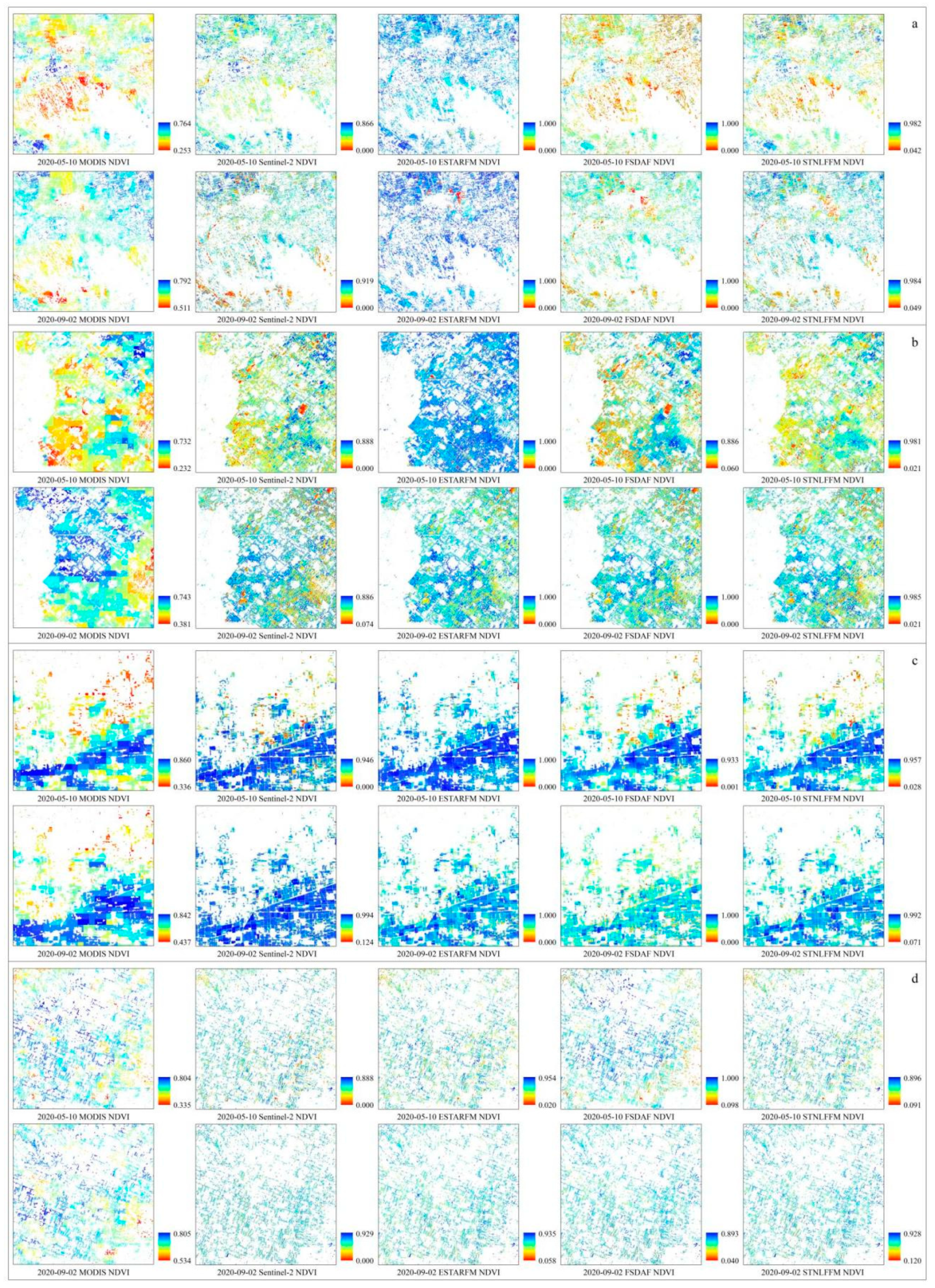
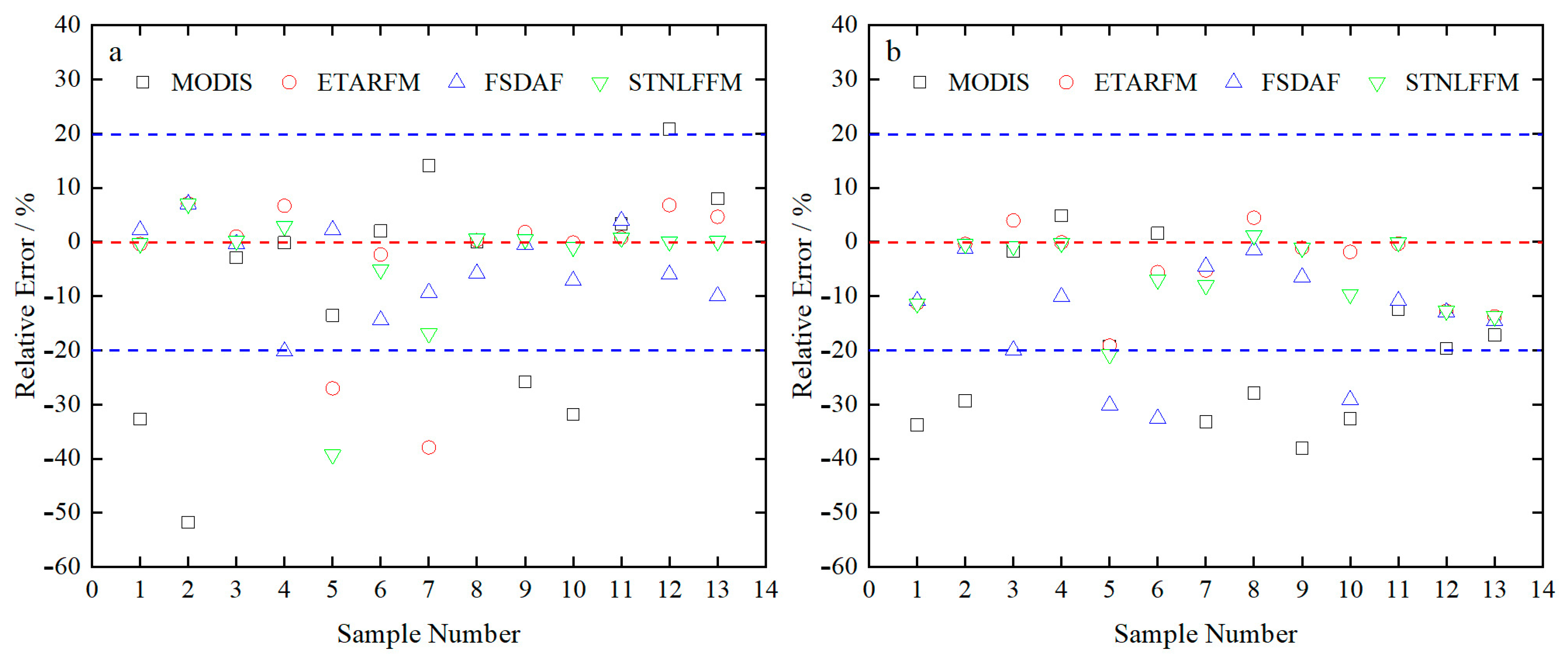
3.1. Accuracy Evaluation of Different Spatiotemporal Fusion Models

The NDVI data (10 m and 1 d) were calculated with ESTARFM, FSDAF, and STNLFFM in the Yuncheng Basin. By comparing the NDVI simulated with ESTARFM, FSDAF, and STNLFFM with Sentinel-2–NDVI at the corresponding time (Figure 3), the overall fusion effect of ESTARFM–NDVI, FSDAF–NDVI, and STNLFFM–NDVI was good. However, the simulated NDVI was poor in the Fenhe River basin and salt ponds in the Xiechi Lake, and the null NDVI was simulated to zero. Moreover, the simulation error of FSDAF–NDVI in the mountainous area along the Zhongtiao Mountains was large on 2 September 2020. While on 24 June, FSDAF–NDVI was small in the summer maize planting area of Xia County and Wenxi County. On this basis, the correlation coefficients, bias, and root mean square errors (RMSE) of ESTARFM–NDVI, FSDAF–NDVI, STNLFFM–NDVI, and Sentinel-2–NDVI at different times were calculated, and the results were shown in Figure 4. Most of the scattered points were mainly concentrated near the y = x line, indicating that the dispersion degree of the fusion image was low, the fusion result was good, and the fused images based on the three models could be used for subsequent yield estimation research. Among them, the scattered points of the STNLFFM model were evenly distributed on both sides of y = x, and the correlation coefficient ranged from 0.791 to 0.881 (p < 0.01), with an average value of 0.831. The bias was between −0.123 and −0.003, and the RMSE were all less than 0.167. The fusion accuracy of the ESTARFM model was second; the maximum and minimum correlation coefficients were 0.876 and 0.771, respectively. The average correlation coefficient was 0.822. The deviation varied between −0.140 and 0.005, while the RMSE ranged from 0.098 to 0.181. The correlation coefficient between FSDAF–NDVI and Sentinel-NDVI exhibited the lowest value, ranging from 0.634 to 0.852, with an average of approximately 0.723. The bias was between −0.090 and 0.018, and the RMSE was 0.15.

The summer maize planting area of the upper, middle, and lower reaches of the Sushui River Basin and Wanrong County were selected for the analysis of MODIS–NDVI, ESTARFM–NDVI, FSDAF–NDVI, STNLFFM–NDVI, and Sentinel-2–NDVI on 10 May, and 2 September 2020 (Figure 5). The spatial details of ESTARFM–NDVI, FSDAF–NDVI, and STNLFFM–NDVI were better than MODIS–NDVI, and could better express the spatial differences among small ground objects. Moreover, MODIS–NDVI, in different summer maize planting areas, was affected by low spatial resolution. There were many mixed pixels, which could not accurately represent the change trend of NDVI in the sample area, and the range of NDVI was small (Figure S1). Further comparison and analysis of ESTARFM–NDVI, FSDAF–NDVI, and STNLFFM–NDVI showed that FSDAF–NDVI had a poor simulation effect in the summer maize planting area at the upper reaches of the Sushui River, and the tonal difference between FSDAF–NDVI and Sentinel-2–NDVI was great. The simulated NDVI value was lower than Sentinel-2–NDVI, and there were a lot of zeros in FSDAF–NDVI in the central area of the Wenxi County, which was inconsistent with the reality. Significant differences between the ESTARFM–NDVI and the contemporaneous Sentinel-2–NDVI were found in the middle and lower part of the Sushui River. The upper limit of FSDAF–NDVI, on 22 October, was less accurate than other fusion models, and the applicability of FSDAF–NDVI in this period was poor (Figure S2). STNLFFM–NDVI had a high simulation effect in the whole basin, and its NDVI range was consistent with Sentinel-2–NDVI. In the Wanrong County, which was far away from the Sushui River Basin, the NDVI texture features simulated by the three spatiotemporal fusion models were clear and consistent with the changes of Sentinel-2–NDVI. Thus, the fusion models of STARFM, FSDAF, and STNLFFM both had strong applicability to simulate NDVI in the Yuncheng Basin, and the simulation accuracy of STNLFFM–NDVI, ESTARFM–NDVI, and FSDAF–NDVI was in order from high to low. The simulation accuracy of STNLFFM–NDVI in the Sushui River Basin was significantly higher than that of ESTARFM–NDVI and FSDAF–NDVI, while the spatial characteristics of summer maize NDVI, based on the three fusion model, were consistent with the changes of contemporaneous Sentinel-2–NDVI in the area far from the Sushui River.

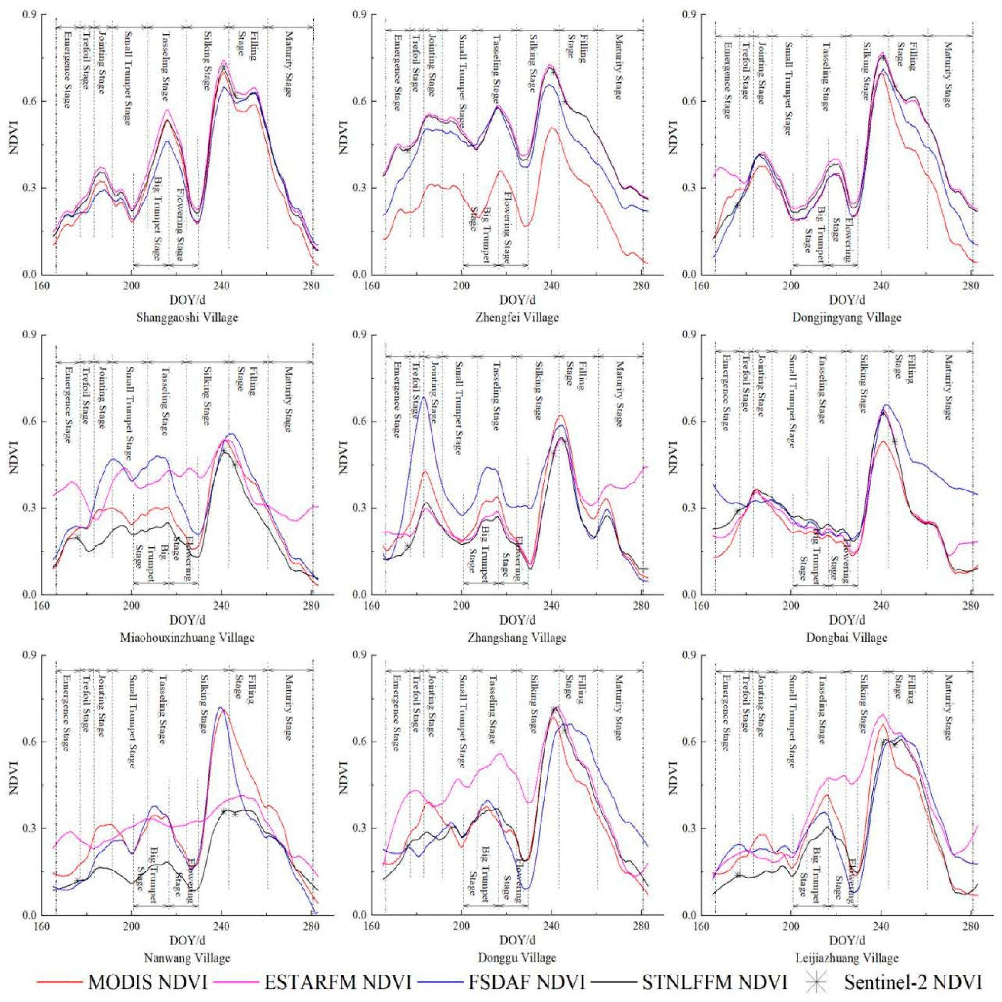
3.2. Analysis of NDVI Growing Curves of Summer Maize in Main Growing Period

Nine summer maize samples were selected. The Savitzky–Golay filter (S–G filter) was used to smooth the MODIS–NDVI, ESTARFM–NDVI, FSDAF–NDVI, and STNLFFM–NDVI data of the nine summer maize samples. The change curves of MODIS–NDVI, ESTARFM–NDVI, FSDAF–NDVI, and STNLFFM–NDVI were obtained (Figure 6). The NDVI time-series curves based on the different data sources showed the same trend in the main growth stage of summer maize (June to September), including small and large waves [39]. Wavelet peaks were observed in DOY217, corresponding to the tasseling of summer maize, occurring between the stage of large trumpet and the flowering. At this stage, the length of spikelets in the middle and upper parts of the main shaft was 0.8 cm, and the bar trefoil flared out in a trumpet shape. The large wave peak appeared at about DOY240, corresponding to the drawing-filling stage of summer maize. Before the drawing–filling stage, all the leaves of summer maize were unfolded, the plants were fixed in height, and NDVI reached the peak. After that, the stem and leaf decay occurred, and NDVI showed a significantly decline trend [11,40]. MODIS–NDVI was greatly affected by mixed pixels and had no significant response to vegetation information that changed in a short time. At the same time, MODIS–NDVI showed low NDVI in most sample points. The fusion methods of ESTARFM, FSDAF, and STNLFFM could improve the low NDVI on the basis of the full consideration of Sentinel-2–NDVI. The time-series NDVI based on STNLFFM could clearly express each growing stage of summer maize, which was close to the contemporaneous Sentinel-2–NDVI. It corresponded to the actual planting date and harvest date, which was more in line with the actual cultivation situation. The error between FSDAF–NDVI in the Zhengfei Village, Dongbai Village, Nanwang Village, and Donggu Village and the contemporaneous Sentinel-2–NDVI was large. The ESTARFM–NDVI curve does not change significantly before the actual planting date, while the STNLFFM–NDVI curve showed a significant decline trend before the actual planting date, and the latter was more consistent with the change trend of the realistic winter wheat-summer maize rotation pattern. Hence, it is widely accepted that STNLFFM–NDVI has the ability to effectively depict the prolonged fluctuation pattern and specific alterations in NDVI, aligning perfectly with the growth attributes of summer maize and fulfilling the criteria for discerning crop cultivation patterns.

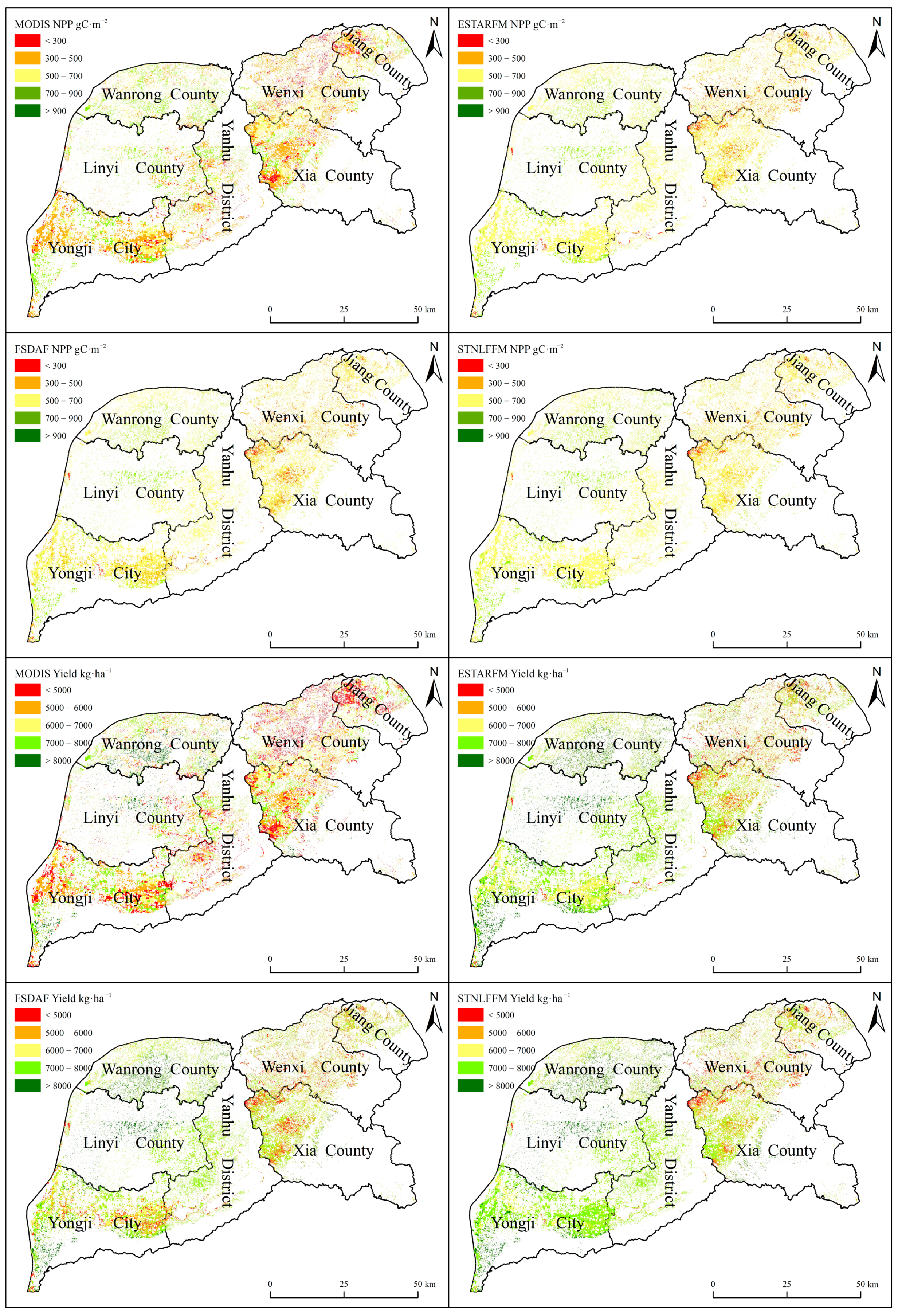
3.3. Results of NPP Simulation and Yield Estimation

The cumulative NPP during the growing period of summer maize was calculated with the CASA model, based on MODIS–NDVI, ESTARFM–NDVI, FSDAF–NDVI, and STNLFFM–NDVI. Yield estimation of summer maize was calculated with the light use efficiency model (Figure 7). In the summer maize planting area of the Yuncheng basin, the cumulative NPP based on MODIS, ESTARFM, FSDAF–NDVI, and STNLFFM were 417.71 gC·m⁻², 494.59 gC·m⁻², 483.16 gC·m⁻², and 500.45 gC·m⁻², respectively. The average summer maize yields in 2020 in the Yuncheng Basin were as follows: MODIS of 5480.63 kg·ha⁻¹, ESTARFM of 6496.11 kg·ha⁻¹, FSDAF of 6363.55 kg·ha⁻¹, and STNLFFM of 6592.95 kg·ha⁻¹, respectively. The NPP of summer maize based on the different data showed the same spatial distribution characteristics: that the NPP was in the Sushui River alluvial plain in the northwest and bordering the Guanzhong Plain in the southwest was significantly higher than that in the mountainous area in the northeast and the northern terrace. ESTARFM–NPP, FSDAF–NPP and STNLFFM–NPP were concentrated in 500–700 gC·m⁻², accounting for more than 70% in the summer maize planting area, among which STNLFFM–NPP accounted for the largest proportion (76.11%). The MODIS–NPP occupied 75.31% in the interval of less than 500 gC·m⁻² and more than 700 gC·m⁻², which was significantly different from ESTARFM–NPP, FSDAF–NPP, and STNLFFM–NPP. The summer maize yield i aligned with the spatial distribution of NPP. The yield estimated that ESTARFM–NDVI, FSDAF–NDVI, and STNLFFM–NDVI accounted for 75.57%, 71.66%, and 76.00%, respectively, while the yield estimated with MODIS–NDVI accounted for only 35.50% in the area. The yield calculated with MODIS–NDVI was low in the Yuncheng Basin.

The estimated summer maize yields obtained from MODIS–NDVI, ESTARFM–NDVI, FSDAF–NDVI, and STNLFFM–NDVI were compared to the measured values (Figure 8). The findings revealed that there was no significant correlation (p > 0.05) between the predicted value based on MODIS–NDVI and the measured value. The absolute error (AE) ranged from −355.59 to 1343.33 kg·ha⁻¹, and the mean absolute percentage error (MAPE) was 18.42%. The correlation coefficient between forecasted yield and measured yield, based on FSDAF–NDVI, was 0.644 (p < 0.01), and the AE ranged from −2533.5 to 483.10. The MAPE was reduced by 7.90% compared to MODIS–NDVI, indicating that the error of summer maize yield forecast based on MODIS–NDVI was large, and the fusion of the Sentinel-2 and MODIS data based on FSDAF could improve the estimation accuracy of summer maize yield per unit area. The correlation coefficients predicted yield and measured yield based on ESTARFM–NDVI and STNLFFM–NDVI and were 0.703 (p < 0.01) and 0.742 (p < 0.01), respectively. The relative error (RE) of the former was between −37.91% and 7.11%, and the RE of the latter was between −39.29% and 7.01%. MAPE was 6.80% and 6.22%, respectively, indicating that the yield prediction accuracy of ESTARFM–NDVI and STNLFFM–NDVI was higher than that of FSDAF–NDVI. The Yuncheng Basin is located at the intersection of semi-arid and semi-humid areas in the southeast of the Loess Plateau. The measured yield of summer maize samples in the semi-humid areas was significantly higher than that in the semi-arid areas. In semi-arid areas, the correlation coefficients predicted yield based on ESTARFM–NDVI, FSDAF–NDVI, and STNLFFM–NDVI, and the measured yield were 0.791, 0.742, and 0.821, respectively. They were higher than the correlation coefficients in the semi-humid areas (0.671, 0.604, 0.677), and were all significant at the level of 0.01. The MAPE between estimated yield based on ESTARFM–NDVI, FSDAF–NDVI, STNLFFM–NDVI and the measured yield in semi-arid areas were 7.46%, 6.48%, and 5.76%, respectively, which were lower than those in semi-humid areas (6.14%, 14.20%, and 6.69%, respectively). It indicated that the yield estimation accuracy of STNLFFM–NDVI in different climatic zones remained high. The yield estimation accuracy of FSDAF–NDVI in semi-arid areas was significantly better than that in semi-humid areas. The yield estimation accuracy based on fusion models in descending order was as follows: STNLFFM, ESTARFM, and FSDAF.

4. Discussion

The Sentinel-2 data can be spatially fused at the corresponding time based on the ESTARFM, FSDAF, and STNLFFM spatiotemporal fusion models. The problem of mixed pixels in the MODIS–NDVI and erroneous NDVI variations can be mostly solved with the Sentinel-2’s geographic details. The accuracy of the NDVI curve simulation and yield estimation of sample points in the main growth period of summer maize are greatly improved. Meanwhile, compared with the fusion of the Landsat and MODIS data, Sentinel-2 has higher spatial resolution than the Landsat data, which is suitable for the Yuncheng Basin, where the topography is fragmented, resulting in the high accuracy of monitoring surface vegetation cover and change. Thus, the application of the Sentinel-2 and MODIS data based on ESTARFM, FSDAF, and STNLFFM to the summer maize planting area in the Southeast Loess Plateau has a good effect. It is found that the parameter settings of different fusion models have a great influence on the fusion effect, and the accuracy of the FADSF model is greatly affected by the window size. When the window size is consistent with ESTARFM and STNLFFM, the residual error in predicting complex ground objects will be too large [33,35], resulting in a large error in the simulation results in the transition zone from forest and grass to cultivated land. Moreover, the FADSF fusion model based on a single high- and low-resolution image has the problem of insufficient robustness, when there are many outliers in the pixels [32,41,42], resulting in spectral distortion and texture blurring of FADSF–NDVI in the summer maize planting area from August to September. Since the ESTARFM fusion method requires two groups of data corresponding to high and low spatial resolution, the weight calculation will be affected and the time–phase relationship will be maintained with a large deviation. In the two groups of corresponding high- and low-spatial-resolution data, the input time terminal significantly increases. Thus, the fusion based on the ESTARFM result has a large error when the gap period of the high-resolution data is long [32,43]. It is also the main reason why the ESTARFM–NDVI curve has a large error at the seedling stage and maturity stage. The STNLFFM algorithm fully considers the conversion coefficient between the different data, and abandons the spectral difference factor and spatial distance factor when constructing weights, while retaining only the time–phase difference factor [32], which is very necessary to improve the fusion accuracy of NDVI, LST, ET, and other index parameters. In order to avoid the decrease of fusion accuracy due to the large difference between the auxiliary time phase and the predicted time phase, the overall weight constructed based on non-local mean filtering is introduced to improve the poor fusion results caused by the long void period of the high-resolution data in the ESTARFM model [11,33]. Thus, the fitting degree of the NDVI curve in the summer maize planting area of the three fusion methods was STNLFFM, ESTARFM, and FADSF in order from high to low.

Affected by terrain and climate, the terrain fragmentation in the northeastern mountainous area and the northern tableland of the Yuncheng Basin is relatively high, which enables an easy formation of soil erosion and hinders the accumulation of NPP. In the western summer maize planting area, the terrain is flat, the land is fertile, and the water and heat conditions are ideal, which is conducive to the growth and development of food crops. The accumulation of NPP is higher, and the yield of summer maize is significantly higher than that in the northeast and northern area [11]. Affected by frequent precipitation in summer [38], the spatial heterogeneity in the semi-humid areas is enhanced, and downscaling (only with resampling in FSDAF) may lead to the same pixel values between adjacent pixels [31,42], resulting in an inaccurate FADSF–NDVI simulation, which leads to large errors in yield estimation. The STNLFFM and ESTARFM fusion models based on two high/low resolution images improve the accuracy of similar pixel screening [30,32], and alleviate the simulation errors caused with enhanced spatial heterogeneity. Thus, the FADSF fusion model has poor adaptability in the semi-humid summer maize planting area. In the semi-arid areas, the yield estimation accuracy of the three fusion models is good; however, considering the characteristics of the FADSF fusion model with less input data and a faster response speed, we believe that it has good adaptability in the semi-arid summer maize planting area.

The theory of the spatiotemporal fusion model based on reconstruction is relatively simple and has strong operability; however, the calculation of weight function relies too much on the pixel information of input images. The fusion results are poor when the time gap of a high-resolution image is long or the quality of a low-resolution image is poor [21,44]. In future research, we should consider using machine learning algorithms to investigate the non-linear relationship between images with different resolutions, and to build a model according to this, obtaining high spatial and temporal resolution images with high precision. Moreover, we should consider the fusion of two or more kinds of sensor data, while making full use of data information from different sources. It is helpful to reduce the differences between different sensor data, combine the advantages of the different data, and improve the fusion effect. The main parameters of the summer maize yield estimation model based on the light use efficiency model, such as the water content coefficient and conversion coefficient, were obtained through sample surveys, and the representation of parameters in the regional scale was poor. Thus, we should focus on achieving a regionalization of parameters, such as using crop models for regional scale parameter inversion [45], and establishing a model based on deep learning that would eventually build a relationship between the primary parameters and spectral indicators.

5. Conclusions

The NDVI data with a spatial resolution of 10 m and a temporal resolution of 1 day were obtained with the spatiotemporal fusion model. In addition to the spatial signatures of Sentinel-2–NDVI, these data could be used to reflect the temporary variation information of MODIS–NDVI. They also solved the poor adaptability of MODIS–NDVI in fragmentation areas with a high degree of terrain. The integration of ESTARFM–NDVI, FSDAF–NDVI, and STNLFFM–NDVI could correctly reflect the local variation information and variation trend of summer maize, which was in line with the growth traits of summer maize in the Yuncheng Basin.

Compared with FSDAF, the fusion accuracy of the ESTARFM and STNLFFM models was good, based on the spatial and texture features of the NDVI data and the results of quantitative statistical analysis. Moreover, the STNLFFM model introduced the overall weight based on non-local mean filtering, which improved the poor fusion results caused by the long gap period of the high-resolution data in the ESTARFM model. The STNLFFM–NDVI could provide data support for accurate monitoring of summer maize growth and accurate yield estimation in the Yuncheng Basin.

The accuracy of the yield estimation model based on the light use efficiency model was as follows: STNLFFM–NDVI (R = 0.742, MAPE = 6.22%), ESTARFM–NDVI (R = 0.703, MAPE = 6.80%), and FSDAF–NDVI (R = 0.644, MAPE = 10.52%). In the semi-arid areas, the yield simulation error based on the FADSF model was small, the amount of model input data was small, and the response speed of the model was fast. The high-precision yield estimation model is essential for timely production strategy modifications and guaranteeing national food security.

References

1. Peng, X.S.; Han, W.T.; Ao, J.Y.; Wang, Y. Assimilation of LAI Derived from UAV Multispectral Data into the SAFY Model to Estimate Maize Yield. Remote Sens. 2021, 13, 1094. [Google Scholar] [CrossRef]
2. Zhang, S.; Bai, Y.; Zhang, J.H.; Ali, S. Developing a process-based and remote sensing driven crop yield model for maize (PRYM-Maize) and its validation over the Northeast China Plain. J. Integr. Agric. 2021, 20, 408–423. [Google Scholar] [CrossRef]
3. Yang, F.; Zhang, D.F.; Zhang, Y.Q.; Zhang, Y.; Han, Y.Y.; Zhang, Q.S.; Zhang, Q.; Zhang, C.H.; Liu, Z.Q.; Wang, K.Y. Prediction of corn variety yield with attribute-missing data via graph neural network. Comput. Electron. Agric. 2023, 211, 108046. [Google Scholar] [CrossRef]
4. Cheng, J.P.; Han, S.Y.; Verrelst, J.; Zhao, C.J.; Zhang, N.; Zhao, Y.; Lei, L.; Wang, H.; Yang, G.J.; Yang, H. Deciphering maize vertical leaf area profiles by fusing spectral imagery data and a bell-shaped function. Int. J. Appl. Earth Obs. Geoinf. 2023, 120, 103355. [Google Scholar] [CrossRef]
5. Zhu, B.X.; Chen, S.B.; Xu, Z.Y.; Ye, Y.H.; Han, C.; Lu, P.; Song, K.S. The Estimation of Maize Grain Protein Content and Yield by Assimilating LAI and LNA, Retrieved from Canopy Remote Sensing Data, into the DSSAT Model. Remote Sens. 2023, 15, 2576. [Google Scholar] [CrossRef]
6. Peng, M.M.; Han, W.T.; Li, C.Q.; Yao, X.M.; Shao, G.M. Modeling the daytime net primary productivity of maize at the canopy scale based on UAV multispectral imagery and machine learning. J. Clean. Prod. 2022, 367, 133041. [Google Scholar] [CrossRef]
7. Wang, P.J.; Wu, D.; Yang, J.Y.; Ma, Y.P.; Feng, R.; Huo, Z.G. Summer maize growth under different precipitation years in the Huang-Huai-Hai Plain of China. Agric. For. Meteorol. 2020, 285, 107927. [Google Scholar] [CrossRef]
8. Zhang, Y.; Gurung, R.; Marx, E.; Williams, S.; Ogle, S.M.; Paustian, K. DayCent model predictions of NPP and grain yields for agricultural lands in the contiguous US. J. Geophys. Res. Biogeosci. 2020, 125, e2020JG005750. [Google Scholar] [CrossRef]
9. Dhillon, M.S.; Dahms, T.; Kuebert-Flock, C.; Borg, E.; Conrad, C.; Ullmann, T. Modelling Crop Biomass from Synthetic Remote Sensing Time Series: Example for the DEMMIN Test Site, Germany. Remote Sens. 2020, 12, 1819. [Google Scholar] [CrossRef]
10. Jackson, H.; Prince, S.D. Degradation of net primary production in a semiarid rangeland. Biogeosciences 2016, 13, 4721–4734. [Google Scholar] [CrossRef]
11. Wang, J.S.; He, P.; Liu, Z.C.; Jing, Y.D.; Bi, R.T. Yield estimation of summer maize based on multi-source remote-sensing data. Agron. J. 2022, 114, 3389–3406. [Google Scholar] [CrossRef]
12. Meraj, G.; Kanga, S.; Ambadkar, A.; Kumar, P.; Singh, S.K.; Farooq, M.; Johnson, B.A.; Rai, A.; Sahu, N. Assessing the yield of wheat using satellite remote sensing-based machine learning algorithms and simulation modeling. Remote Sens. 2022, 14, 3005. [Google Scholar] [CrossRef]
13. Shi, S.; Ye, Y.; Xiao, R. Evaluation of food security based on remote sensing data—Taking Egypt as an example. Remote Sens. 2022, 14, 2876. [Google Scholar] [CrossRef]
14. Yu, D.; Shi, P.; Shao, H.; Zhu, W.; Pan, Y. Modelling net primary productivity of terrestrial ecosystems in East Asia based on an improved CASA ecosystem model. Int. J. Remote Sens. 2009, 30, 4851–4866. [Google Scholar] [CrossRef]
15. Zhou, Y.; Wu, X.; Ju, W.; Chen, J.M.; Wang, S.; Wang, H.; Yuan, W.; Andrew Black, T.; Jassal, R. Global parameterization and validation of a two-leaf light use efficiency model for predicting gross primary production across FLUXNET sites. J. Geophys. Res. Biogeosci. 2016, 121, 1045–1072. [Google Scholar] [CrossRef]
16. Xiao, F.; Liu, Q.; Xu, Y. Estimation of terrestrial net primary productivity in the Yellow River Basin of China using light use efficiency model. Sustainability 2022, 14, 7399. [Google Scholar] [CrossRef]
17. Liu, Y.; Han, X.; Weng, F.; Xu, Y. Estimation of terrestrial net primary productivity in China from Fengyun-3D satellite data. J. Meteorol. Res. 2022, 36, 401–416. [Google Scholar] [CrossRef]
18. Kastner, T.; Erb, K.H.; Haberl, H. Global human appropriation of net primary production for biomass consumption in the European Union, 1986–2007. J. Ind. Ecol. 2015, 19, 825–836. [Google Scholar] [CrossRef]
19. Ji, F.; Meng, J.; Cheng, Z.; Fang, H.; Wang, Y. Crop yield estimation at field scales by assimilating time series of Sentinel-2 data into a modified CASA-WOFOST coupled model. IEEE Trans. Geosci. Remote Sens. 2021, 60, 4400914. [Google Scholar] [CrossRef]
20. Pott, L.P.; Amado, T.J.C.; Schwalbert, R.A.; Corassa, G.M.; Ciampitti, I.A. Mapping crop rotation by satellite-based data fusion in Southern Brazil. Comput. Electron. Agric. 2023, 211, 109758. [Google Scholar] [CrossRef]
21. Wang, Z.; Ma, Y.; Zhang, Y. Review of pixel-level remote sensing image fusion based on deep learning. Inf. Fusion 2023, 90, 36–58. [Google Scholar] [CrossRef]
22. Yang, G.; Weng, Q.; Pu, R.; Gao, F.; Sun, C.; Li, H.; Zhao, C. Evaluation of ASTER-like Daily Land Surface Temperature by Fusing ASTER and MODIS Data during the HiWATER-MUSOEXE. Remote Sens. 2016, 8, 75. [Google Scholar] [CrossRef]
23. Yang, Y.; Anderson, M.C.; Gao, F.; Hain, C.R.; Semmens, K.A.; Kustas, W.P.; Noormets, A.; Wynne, R.H.; Thomas, V.A.; Sun, G. Daily Landsat-scale evapotranspiration estimation over a forested landscape in North Carolina, USA, using multi-satellite data fusion. Hydrol. Earth Syst. Sci. 2017, 21, 1017–1037. [Google Scholar] [CrossRef]
24. Malenovský, Z.; Bartholomeus, H.M.; Acerbi-Junior, F.W.; Schopfer, J.T.; Painter, T.H.; Epema, G.F.; Bregt, A.K. Scaling dimensions in spectroscopy of soil and vegetation. Int. J. Appl. Earth Obs. Geoinf. 2007, 92, 137–164. [Google Scholar] [CrossRef]
25. Liu, M.; Ke, Y.; Yin, Q.; Chen, X.; Im, J. Comparison of five spatio-temporal satellite image fusion models over landscapes with various spatial heterogeneity and temporal variation. Remote Sens. 2019, 11, 2612. [Google Scholar] [CrossRef]
26. Yang, J.; Zhao, Y.Q.; Chan, J.C.W. Hyperspectral and multispectral image fusion via deep two-branches convolutional neural network. Remote Sens. 2018, 10, 800. [Google Scholar] [CrossRef]
27. Jarihani, A.A.; McVicar, T.R.; Van Niel, T.G.; Emelyanova, I.V.; Callow, J.N.; Johansen, K. Blending Landsat and MODIS Data to Generate Multispectral Indices: A Comparison of “Index-then-Blend” and “Blend-then-Index” Approaches. Remote Sens. 2014, 6, 9213–9238. [Google Scholar] [CrossRef]
28. Jiang, X.; Huang, B. Unmixing-based spatiotemporal image fusion accounting for complex land cover changes. IEEE Trans. Geosci. Remote Sens. 2022, 60, 5623010. [Google Scholar] [CrossRef]
29. Gao, F.; Masek, J.; Schwaller, M.; Hall, F. On the blending of the Landsat and MODIS surface reflectance: Predicting daily Landsat surface reflectance. IEEE Trans. Geosci. Remote Sens. 2006, 44, 2207–2218. [Google Scholar]
30. Knauer, K.; Gessner, U.; Fensholt, R.; Kuenzer, C. An ESTARFM fusion framework for the generation of large-scale time series in cloud-prone and heterogeneous landscapes. Remote Sens. 2016, 8, 425. [Google Scholar] [CrossRef]
31. Zhu, X.; Helmer, E.H.; Gao, F.; Liu, D.; Chen, J.; Lefsky, M.A. A flexible spatiotemporal method for fusing satellite images with different resolutions. Remote Sens. Environ. 2016, 172, 165–177. [Google Scholar] [CrossRef]
32. Dong, S.; Zhang, W.; Xu, J.; Ma, J. Study of the Improved Similar Pixel Selection Method on ESTARFM. Remote Sens. Technol. Appl. 2020, 35, 185–193. [Google Scholar]
33. Lei, C.Y.; Meng, X.C.; Shao, F. Spatio-temporal fusion quality evaluation based on “Point”-“Line”-“Plane” aspects. Natl. Remote Sens. Bull. 2021, 25, 791–802. [Google Scholar] [CrossRef]
34. Hobyb, A.; Radgui, A.; Tamtaoui, A.; Er-Raji, A.; El Hadani, D.; Merdas, M.; Smiej, F.M. Evaluation of spatiotemporal fusion methods for high resolution daily NDVI prediction. In Proceedings of the Multimedia Computing and Systems of the International Conference, Marrakech, Morocco, 29 September 2016. [Google Scholar]
35. Fan, M.; Ma, D.; Huang, X.; An, R. Adaptability Evaluation of the Spatiotemporal Fusion Model ofSentinel-2 and MODIS Data in a Typical Area of the Three-River Headwater Region. Sustainability 2023, 15, 8697. [Google Scholar] [CrossRef]
36. Yin, X.; Zhu, H.; Gao, J.; Gao, J.; Guo, L.; Gou, Z. NPP Simulation of Agricultural and Pastoral Areas Based on Landsat and MODIS Data Fusion. Trans. Chin. Soc. Agric. Mach. 2020, 51, 163–170. [Google Scholar]
37. He, P.; Bi, R.; Xu, L.; Liu, Z.; Yang, F.; Wang, W.; Cui, Z.; Wang, J. Evapotranspiration of Winter Wheat in the Semi-Arid Southeastern Loess Plateau Based on Multi-Source Satellite Data. Remote Sens. 2023, 15, 2095. [Google Scholar] [CrossRef]
38. Sun, C.; Chen, W.; Chen, Y.; Cai, Z. Stable isotopes of atmospheric precipitation and its environmental drivers in the Eastern Chinese Loess Plateau, China. J. Hydrol. 2020, 581, 124404. [Google Scholar] [CrossRef]
39. Zhang, F.; Chen, Y.; Zhang, J.; Guo, E.; Wang, R.; Li, D. Dynamic drought risk assessment for maize based on crop simulation model and multi-source drought indices. J. Clean. Prod. 2019, 233, 100–114. [Google Scholar] [CrossRef]
40. Guo, X.; Li, G.H.; Ding, X.P.; Zhang, J.W.; Ren, B.Z.; Liu, P.; Zhang, S.G.; Zhao, B. Response of leaf senescence, photosynthetic characteristics, and yield of summer maize to controlled-release urea based application depth. Agronomy 2022, 12, 687. [Google Scholar] [CrossRef]
41. Liu, M.; Yang, W.; Zhu, X.; Chen, J.; Chen, X.; Yang, L.; Helmer, E.H. An Improved Flexible Spatiotemporal DAta Fusion (IFSDAF) method for producing high spatiotemporal resolution normalized difference vegetation index time series. Remote Sens. Environ. 2019, 227, 74–89. [Google Scholar] [CrossRef]
42. Zhang, H.W.; Huang, F.; Hong, X.C.; Wang, P. A Sensor Bias Correction Method for Reducing the Uncertainty in the Spatiotemporal Fusion of Remote Sensing Images. Remote Sens. 2022, 14, 327. [Google Scholar] [CrossRef]
43. Dhillon, M.S.; Kübert-Flock, C.; Dahms, T.; Rummler, T.; Arnault, J.; Steffan-Dewenter, I.; Ullmann, T. Evaluation of MODIS, Landsat 8 and Sentinel-2 Data for Accurate Crop Yield Predictions: A Case Study Using STARFM NDVI in Bavaria, Germany. Remote Sens. 2023, 15, 1830. [Google Scholar] [CrossRef]
44. Li, X.; Liang, S.; Jin, H. An Effective Method for Generating Spatiotemporally Continuous 30 m Vegetation Products. Remote Sens. 2021, 13, 719. [Google Scholar] [CrossRef]
45. Xie, Y.; Huang, J. Integration of a Crop Growth Model and Deep Learning Methods to Improve Satellite-Based Yield Estimation of Winter Wheat in Henan Province, China. Remote Sens. 2021, 13, 4372. [Google Scholar] [CrossRef]
Figure 1. The geographical location of the study area, spatial distribution of meteorological stations and sampling locations, precipitation, temperature, and total solar radiation during the growing period of summer maize.
Agronomy 13 02608 g001
Figure 2. Research framework for accurate rise monitoring and yield estimation in summer maize using fusion and estimation models.
Agronomy 13 02608 g002
Figure 3. NDVI of different periods fused with ESTARM, FSDAF, and STNLFFM, compared with Sentinel-2–NDVI of the Yuncheng Basin in the same time period.
Agronomy 13 02608 g003
Figure 4. Density scatter plots of Sentinel-2–NDVI and the NDVI simulated with ESTARFM, FSDAF, and STNLFFM in different periods.
Agronomy 13 02608 g004
Figure 5. Spatial distribution characteristics of Sentinel-2–NDVI, ESTARFM–NDVI, FSDAF–NDVI, STNLFFM–NDVI, and MODIS–NDVI on 10 May and 2 September 2020, in summer maize planting areas of Yuncheng Basin; parts (ad) represent the upper, middle, and lower reaches of Sushui River Basin and Wanrong County, respectively.
Agronomy 13 02608 g005
Figure 6. MODIS–NDVI, ESTARFM–NDVI, FSDAF–NDVI, and STNLFFM–NDVI growing curves of summer maize fertility period (DOY 160–290) samples based on Savitzky–Golay (S–G) filtering in Zhangshang Village in Jiang County; Dongbai Village and Nanwang Village in Wenxi County; Miahouxinzhuang Village in Xia County; Zhengfei Village and Donggu Village in Yanhu District; Dongjingyang Village in Linyi County; and Shanggao Village and Leizjiazhuang Village in Yongji City.
Agronomy 13 02608 g006
Figure 7. Spatial distribution of NPP accumulation in main growth stages and the yield estimation in the summer maize planting area of Yuncheng Basin in 2020.
Agronomy 13 02608 g007
Figure 8. Parts (a,b) represent the precision comparison between the predicted yield and the measured yield with different models in semi-arid and semi-humid areas, respectively; sample numbers 1–13 of part (a) represent summer maize samples in Cangdi Village, Dongbai Village, Xiguandi Village, Poshen Village, Nanwang Village, Ruyixia Village, Peinan Village, Guodian Village, Nianzhang Village, Shangguo Village, Donggu Village, Zhangshang Village, and MiaohouXin Village; sample numbers 1–13 of part (b) represent summer maize samples in Xiachao Village, Maoying Village, Luche Village, Xixia Village, Beigu Village, Xizhang Village, Pinghao Village, Hanjiazhuang Village 1, Hanjiazhuang Village 2, Leijiazhuang Village, Shanggao Village, Zhengfei Village, and Dongjingyang Village, respectively.
Agronomy 13 02608 g008
Disclaimer/Publisher’s Note: The statements, opinions and data contained in all publications are solely those of the individual author(s) and contributor(s) and not of MDPI and/or the editor(s). MDPI and/or the editor(s) disclaim responsibility for any injury to people or property resulting from any ideas, methods, instructions or products referred to in the content.