Calibration of Small-Grain Seed Parameters Based on a BP Neural Network: A Case Study with Red Clover Seeds

Abstract

In order to enhance the accuracy of discrete element numerical simulations in the processing of small-seed particles, it is essential to calibrate the parameters of seeds within the discrete element software. This study employs a series of physical tests to obtain the physical and contact parameters of red clover seeds. A discrete element model of red clover seeds is established. Plackett–Burman Design, steepest ascent, and Central Composite Design experiments are sequentially conducted. The simulation deviation of the resting angle of red clover seeds is employed as the evaluation criterion for parameter optimization. The results indicate that the coefficients of static friction between red clover seeds, the coefficients of rolling friction between red clover seeds, and the coefficients of static friction between red clover seeds and the steel plates significantly influence the resting angle. Modeling was performed using a backpropagation neural network, a genetic algorithm–optimized BP network, particle swarm optimization, and simulated annealing. It was found that GA-BP ensured both accuracy and stability. Compared to the traditional response surface methodology, GA-BP showed better fitting performance. For the optimized red clover seed simulation, the error between the angle of repose and the physical experiment was 0.98%. This research provides new insights into the calibration of small-grain seed parameters, demonstrating the value of GA-BP for precision modeling.

1. Introduction

Seed processing technology is of significant interest, as it not only enhances seed quality but also paves the way for commercialization. The applications of seed processing technology are diverse, encompassing processes such as seed cleaning [1], coating [2], and sowing [3]. With the advancement of computer numerical simulation techniques, the Discrete Element Method (DEM) has emerged as a crucial approach in the study of seed processing procedures. DEM enables tracking the forces and motions experienced by seeds during processing, unraveling the interplay between the seeds and the machinery, and pinpointing areas for targeted machinery improvements. This can lead to reduced trial periods and costs, showing promising prospects for substantial growth.

Numerous scholars have researched the application of DEM in the realm of agricultural materials. However, the precision of DEM poses certain challenges owing to inaccuracies within simulation models and the intricacies of particle motion. Thus, there arises a necessity to calibrate simulation models. Discrete element simulation experiments require an array of simulation parameters, material properties (such as dimensions, density, thousand-grain weight, Poisson’s ratio, and elastic modulus), and contact parameters (including collision restitution coefficient, static friction coefficient, and rolling friction coefficient) [4]. In light of this, calibration studies have been conducted for discrete element models pertaining to agricultural produce like crop seeds, soil, powders, straw, and potatoes [5]. Wang et al. [6] employed the multisphere- and polyhedron-filling methods to construct different-precision models for sunflower seeds, validating model accuracy through experimentation. Bembenek et al. [7] established a discrete element model for the roller compaction of materials, illustrating the superior applicability of their model compared to finite element methods. Haobaoer et al. [8] devised a coupled simulation model for soil erosion and two-phase flow in arid and semi-arid regions, leading to soil parameter calibration. Liu et al. [9] utilized the Johnson–Kendall–Roberts (JKR) model to calibrate powder simulation parameters, offering subsequent insights for seed coating simulations. Adilet et al. [10] established a nonlinear relationship between dynamic-macroscopic-particle-fertilizer characteristics and DEM parameters. Chen et al. [11] employed the EDEM2020 software to investigate the impact of unit area normal stiffness, unit area shear stiffness, critical normal stress, critical shear stress, and filling sphere radius on the performance of cohesive particle models, proposing a calibration approach for bonded-particle model parameters. Furthermore, Zhang et al. [12] formulated a discrete element model for compacted straw cubes featuring the elastic, plastic, and viscous mechanical properties of flexible straw. Notably, however, limited research has been conducted concerning the calibration of parameters for small-grain forage seeds, given their irregular shape and diminutive size.

In recent years, with the advancement of machine learning techniques, some researchers have utilized technologies such as genetic algorithms and neural networks for model optimization, yielding more accurate results. Traditional response surface methodology (RSM) analysis might encounter complexities and sample size limitations that affect its fitting performance. Compared to traditional multivariate linear regression, the backpropagation (BP) neural network boasts enhanced fitting capabilities, enabling the approximation of intricate nonlinear functions [13]. The multilayer structure of BP neural networks facilitates the extraction of complex nonlinear features from data, mitigating issues of multicollinearity inherent to linear regression and enhancing the reliability of the fitting outcomes. Contrary to the substantial data requirements of conventional machine learning models, studies indicate that after the design of experiments, neural network models can be established with relatively modest datasets [14,15,16,17]. Some researchers have merged BP neural networks with techniques like genetic algorithms for model optimization studies. Tang et al. [18] compared the predictive efficacy of the genetic algorithm–optimized BP (GA-BP) model and the RSM model in cyclone separator design; Liang et al. [19] combined RSM with WOA-BP neural networks to optimize foam separation process parameters, elevating foam separation techniques; and Abdelhalim et al. [20] proposed a hybrid optimization method that amalgamates artificial neural network algorithms with particle swarm optimization (PSO) for predicting cation removal efficiency from aqueous solutions. Owing to their potent nonlinear fitting capabilities, BP neural networks can construct intricate black-box models; PSO algorithms facilitate the effective avoidance of local optima through collective search; and simulated annealing (SA) algorithms employ probabilistic jump techniques to escape local optima. These methodologies, compared to RSM experiments, often yield more precise and robust fitting outcomes. Consequently, embarking on this research holds significance and interest.

Research on the calibration of small-grain seed parameters using BP neural networks is currently limited. This study uses red clover (Trifolium pratense L.) seeds as the research object. Physical experiments are first conducted to obtain red clover seed parameters. A discrete element model of the small-grain seeds is then established in the EDEM software. The error between the angle of repose from the red clover seed simulation experiments and the physical experiments is taken as the response value for the red clover seed parameter calibration experiments. Different machine learning regression models are compared in terms of stability and accuracy. A GA-BP algorithm model is established to determine the optimal combination of simulation parameters for red clover seeds and improve simulation modeling accuracy. This study provides a basis for the calibration of simulation parameters for other small-grained forage seeds.

2. Materials and Methods

2.1. Physical Testing of Red Clover Seed Properties

2.1.1. Determination of Basic Physical Parameters

Red clover seeds were selected as the experimental material for the measurement of readily obtainable basic physical characteristics [21,22]. A random sample of 1000 red clover seeds was taken. The thousand-grain mass of the seeds was measured using an electronic balance with a precision of 0.1 g. The 1000 seeds were divided equally into five groups, and the weight of each group was weighed and multiplied by 5 to obtain the thousand-seed weight. The dimensions (length L × width W × thickness T) of the red clover seeds were measured using a vernier caliper with a precision of 0.02 mm, and the average value of seed dimensions was obtained by repeating the test several times. Their density was measured using a graduated cylinder with a precision of 0.2 mL. The moisture content of the red clover seeds was determined using the oven-drying method (

Table 1. Basic physical properties of Red Clover seed.

Physical Parameters	Red Clover Seeds
Overall dimensions (length L × width W × thickness T) (mm)	L: 2.0 ± 0.125 × W: 1.5 ± 0.054 × T: 1.1 ± 0.062
Thousand-grain mass (g)	1.5 ± 0.156
Density (kg·m−3)	1279 ± 0.035
Moisture content (%)	15 ± 0.352

).

2.1.2. Shear Modulus and Poisson’s Ratio Testing

The shear modulus is the ratio of shear stress to shear strain in a material under shear loading, within the limit of elastic deformation. The Poisson’s ratio is the absolute value of the ratio of transverse contraction strain to axial elongation strain for a material under uniaxial tensile or compressive loading. It is also called the transverse deformation coefficient, reflecting the material’s resistance to lateral deformation [23].

In this study, a professional food texture analyzer (model: TMS-PRO) was utilized to conduct compression and shearing tests on red clover seeds, as illustrated in Figure 1. The shear modulus of the red clover seeds was obtained. The TMS-PRO sensor has a measurement range of 0 to 2.5 kN. For the compression test, the seeds were positioned horizontally and loaded at 15 mm/min for 5 s. For the shear test, a 0.04 mm thick steel plate was used, and seeds were loaded at 15 mm/min until cut after 8 s. Using the software’s post-processing module, load-displacement compression data were obtained. The elastic modulus was calculated via Equation (1), and the shear modulus via Equation (2). Repeated experiments yielded a shear modulus for red clover seeds ranging from 5 to 20 MPa.

$$E=\frac{\sigma }{\epsilon }$$

(1)

$$G_S=\frac{\tau }{\gamma }$$

(2)

where E is the elastic modulus of red clover seeds (Pa); σ is the maximum compressive stress (Pa); ε is the linear strain; G_S is the shear modulus of red clover seeds (Pa); τ is the maximum shear stress (Pa); and γ is the shear strain.

Conventional experimental methods have difficulty determining the Poisson’s ratio of small-grain seeds accurately [24,25]. The Poisson’s ratio (v) of red clover seeds is quantitatively related to the shear modulus and elastic modulus. By deducing from Equation (3), the Poisson’s ratio of red clover seeds can be obtained. Repeated experiments revealed a Poisson’s ratio for red clover seeds ranging from 0.2 to 0.4.

$$v=\frac{E}{2G_S}-1$$

(3)

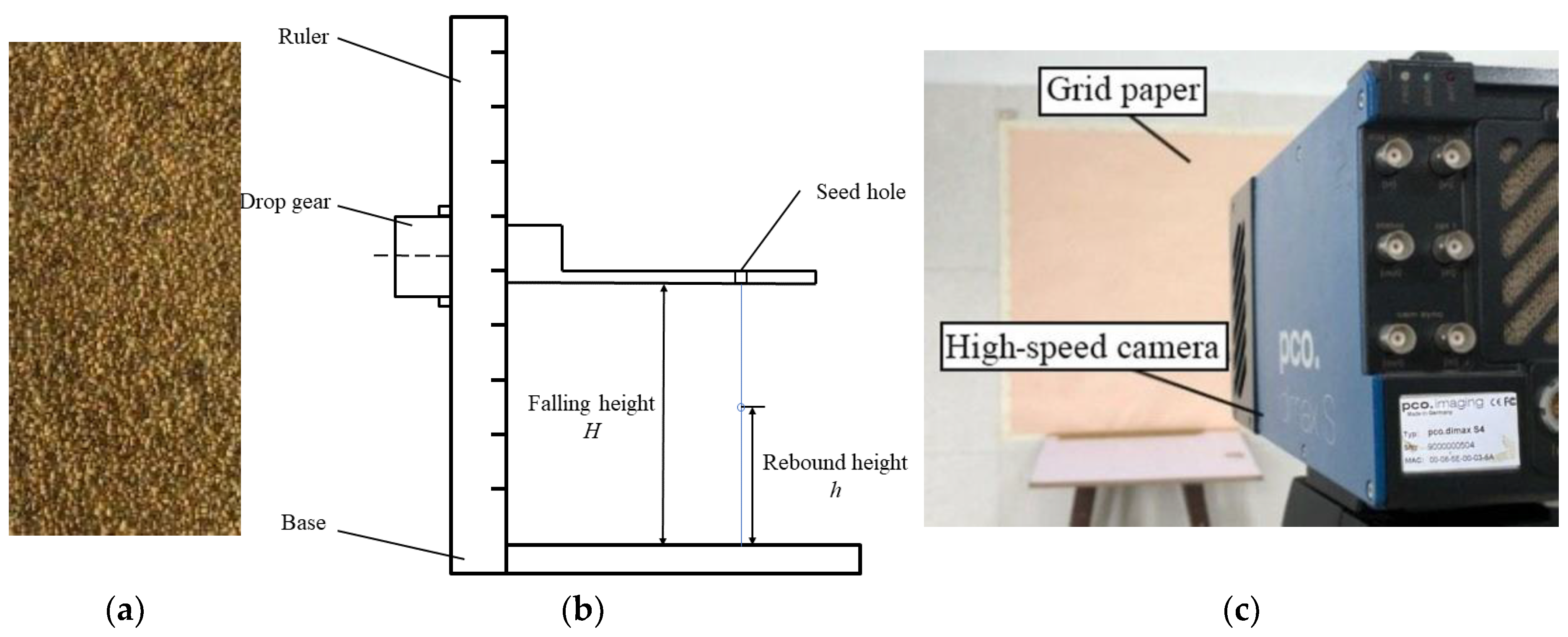
2.1.3. Contact Parameter Testing

The coefficient of restitution measures an object’s ability to recover its original shape after deformation during a collision. It is defined as the ratio of the normal components of the post-collision instantaneous relative velocity to the pre-collision normal approach velocity at the contact point [25,26]. The static friction coefficient is the ratio of the maximum static friction force to the normal contact force between two surfaces [27]. The rolling friction coefficient characterizes the resistance caused by deformation at the contact area when one object rolls or tends to roll on another surface without sliding [28].

A series of contact parameters (coefficient of restitution, static friction coefficient, and rolling friction coefficient) were tested for red clover seed–seed and seed–steel plate interactions relevant to seed processing. To determine the coefficient of restitution between seeds, a seed bed was formed by spreading out a layer of seeds, as shown in Figure 2a. Seeds were released from height H = 150 mm with zero initial velocity to free-fall onto the bed, causing a rebound, as illustrated in Figure 2b. A high-speed PCO.dimax camera captured the falling and rebounding process pictured in Figure 2c. The TEMA3.4-500 software data module analyzed the results. To determine the coefficient with a steel plate, the seed bed was replaced by a plate, and the procedure was repeated. Based on Figure 2b, the coefficient of restitution e is:

$$e=\frac{{v_2}^{\prime }-{v_1}^{\prime }}{v_1-v_2}$$

(4)

where v₂′ is the post-collision velocity of the base plate (m/s); v₁′ is the post-collision velocity of the seed (m/s); v₂ is the pre-collision velocity of the base plate (m/s); and v₁ is the pre-collision velocity of the seed (m/s).

After the free-falling seed collides with the base plate and rebounds, only the gravity of the seed itself does work during the falling and rising motions. Thus, the pre-collision and post-collision velocities of the base plate are both 0, where v₁′ = $\sqrt{2gh}$ and v₁ = $\sqrt{2gH}$. The coefficient of restitution can be simplified as:

$$e=\sqrt{\frac{h}{H}}$$

(5)

where h is the rebound height of the seed (mm); H is the initial drop height of the seed (mm); and g is the acceleration of gravity (m/s²).

By substituting the experimental results into Equation (5), the coefficient of restitution e was obtained. Through repeated tests, the coefficient of restitution for red clover seed–seed collision ranged from 0.4 to 0.6 and for seed–steel plate collision from 0.5 to 0.7.

To determine the static friction coefficient between the seeds and the steel plate, red clover seeds were placed on a CNY-1 inclined plane tester, as shown in Figure 3a. The inclined plane was slowly rotated until the seeds started to slide, at which point the rotation was stopped and the angle recorded. This angle was used in Equation (6) to calculate the static friction factor between the seeds and the steel plate [29]. To obtain the rolling friction coefficient, the plane was further rotated until the seeds rolled, and the indicated angle was again recorded and applied in Equation (7). For seed–seed static and rolling coefficients, the same procedure was followed using a seed bed surface. Through repeated testing, the static friction coefficient for seed–seed ranged from 0.5 to 0.7 and for seed–steel plate from 0.3 to 0.5, while the rolling friction coefficient for seed–seed ranged from 0.6 to 0.8 and for seed–steel plate from 0.2 to 0.5.

$$f_s=\mathit{tan}{\alpha }_1$$

(6)

where f_s represents the static friction coefficient and α₁ denotes the critical angle for static friction in degrees.

$$f_k=\mathit{tan}{\alpha }_2$$

(7)

where f_k stands for the rolling friction coefficient and α₂ signifies the critical angle for rolling friction in degrees.

2.1.4. Resting Angle Testing

The angle of repose is the angle formed between the base plane and the side surface of a conical accumulation of granular material when it naturally falls from a certain height onto a flat surface. This angle reflects the internal friction properties of the material and its behavior during natural scattering. Utilizing the angle of repose test for calibrating particle contact parameters can significantly streamline the DEM modeling process for large-particle systems [30]. The resting angle of red clover seeds was measured using an FT-104B resting angle tester. Seeds were introduced through the feeding port and allowed to free-fall onto the bottom disk, as depicted in Figure 4. Once the seeds came to a complete standstill, an overhead view image of the pile was captured using a high-definition camera. The image underwent grayscale processing, binarization, boundary pixel point extraction, and fitting in Matlab2020b. Through multiple repeated trials, the average resting angle from the physical experiments for red clover seeds was determined to be 24.57°.

2.2. Discrete Element Simulation Model Setup

2.2.1. Creation of Red Clover Seed Simulation Model

A geometric model of the seed particles was developed using three-dimensional modeling software and then converted to STP format before being imported into the EDEM discrete element simulation software. To enhance computational efficiency, the seed model was rounded, and a discrete element simulation model for a red clover seed was established using multiple overlapping spheres. The dimensions of the seed particle model were set according to actual measured values. A total of 9 individual spheres were utilized for filling, with the smallest radius being 0.38 mm, as illustrated in Figure 5.

2.2.2. Setting of Discrete Element Simulation Parameters

Within the EDEM simulations, the Hertz–Mindlin (no-slip) model was selected for the red clover seed particles. A virtual particle plane (Polygon) was established at the instrument funnel outlet to generate the particles. The dynamic generation method generated seeds at 10,000/s, resulting in 2500 total particles. To balance reliability and efficiency, fixed-sized particles were utilized. The total simulation duration was 2 s, with the first 0.25 s allocated for particle generation and the remaining time for particle descent and accumulation. The time step was set to 20% of the Rayleigh time step for numerical stability, with data written every 0.01 s. The mesh size was set to three times the smallest particle radius.

2.3. Calibration of Discrete Element Parameters for Red Clover Seeds

For the calibration of discrete element parameters for red clover seeds, a Plackett–Burman experiment was conducted to screen for significant simulation parameters affecting the response value. Next, a steepest ascent experiment determined the optimal range of the significant parameters. Using a Central Composite Design experiment, a quadratic regression model was developed to predict the relative error between the simulated and physical resting angles. Response surface analysis was then used to analyze the results of the Central Composite Design experiment.

2.3.1. Plackett–Burman Experiment

The parameter range for the Plackett–Burman experiment was based on the physical experiment results. The simulated resting angle of red clover seeds was the response value. The Plackett–Burman experiment identified parameters significantly influencing this response. The minimum and maximum values of the experimental parameters in

Table 2. Plackett–Burman test parameter table.

NO.	Test Parameters	Encoding
		Low (−1)	Middle (0)	High (+1)
A	Seed Poisson’s ratio	0.2	0.3	0.4
B	Seed shear modulus (MPa)	5	12.5	20
C	Seed–seed collision restitution coefficient	0.4	0.5	0.6
D	Seed–steel plate collision restitution coefficient	0.5	0.6	0.7
E	Seed–seed static friction coefficient	0.5	0.6	0.7
F	Seed–steel plate static friction coefficient	0.3	0.4	0.5
G	Seed–seed rolling friction coefficient	0.6	0.7	0.8
H	Seed–steel plate rolling friction coefficient	0.2	0.35	0.5

were encoded as −1 and +1, respectively, where −1 indicated the low parameter level and +1 indicated the high level. After each simulation trial, the resting angle of the seed pile was measured using the same method as in the physical experiments.

2.3.2. Steepest Ascent Experiment

Building upon the Plackett–Burman results, a steepest ascent experiment was performed on the identified significant parameters (red clover seed-to-seed static friction coefficient, seed-to-seed rolling friction coefficient, and seed-to-steel-plate static friction coefficient). The evaluation criterion was the relative error between the simulated and physical resting angles, aiming to establish the optimal range for the parameters [31,32]. In the simulations, nonsignificant parameters were assigned average values from the physical experiments: red clover seed Poisson’s ratio was set to 0.3, shear modulus to 12.5 MPa, seed-to-seed collision restitution coefficient to 0.50, seed-to-steel-plate collision restitution coefficient to 0.57, and seed-to-steel-plate rolling friction coefficient to 0.37.

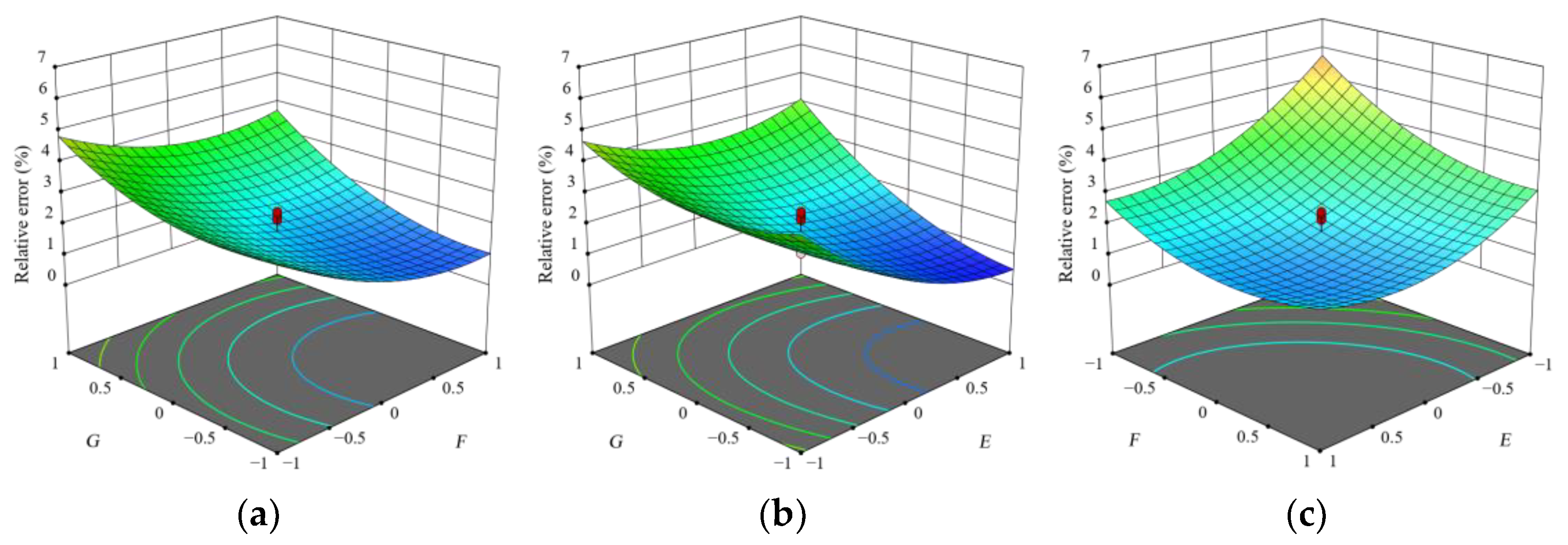
2.3.3. Central Composite Design Experiment

Using point (0) from level 3 of the steepest ascent experiment as the center, levels 2 and 4 were designated as the low (−1) and high (+1) levels, respectively. A Central Composite Design experiment was conducted using the relative error between the simulated and physical resting angles as the evaluation criterion to calibrate the significant red clover seed parameters. The coding of the seed parameter levels is outlined in

Table 3. Level-coding table of parameters.

Levels	Test Parameters
	E	F	G
−1.682	0.513	0.313	0.613
−1	0.54	0.34	0.64
0	0.58	0.38	0.68
+1	0.62	0.42	0.72
+1.682	0.647	0.447	0.747

.

2.4. Regression Modeling Using Machine Learning Algorithms

RSM experiments involve actively collecting data based on multivariate linear regression to obtain regression equations with favorable properties. In recent years, with the advancement of machine learning, modern intelligent optimization algorithms can also perform excellent regression fitting and modeling compared to RSM regression models. The neural network structure consists of interconnected layers of neurons, primarily comprising three layers: input layer, hidden layer, and output layer, as illustrated in Figure 6 [33]. Each layer has neurons connected to the next, passing information up to the output layer. In Figure 6, each input neuron (X) is multiplied by their respective weight (W), added to the bias vector (b), and passed through an activation function (f) to obtain the specific output neuron (a). Using the Central Composite Design experimental results as the dataset, BP, GA-BP, PSO, and SA regression models were constructed for fitting. The dataset (23 sets) was randomly divided into training sets (17 sets, 70%), testing sets (3 sets, 15%), and validation sets (3 sets, 15%).

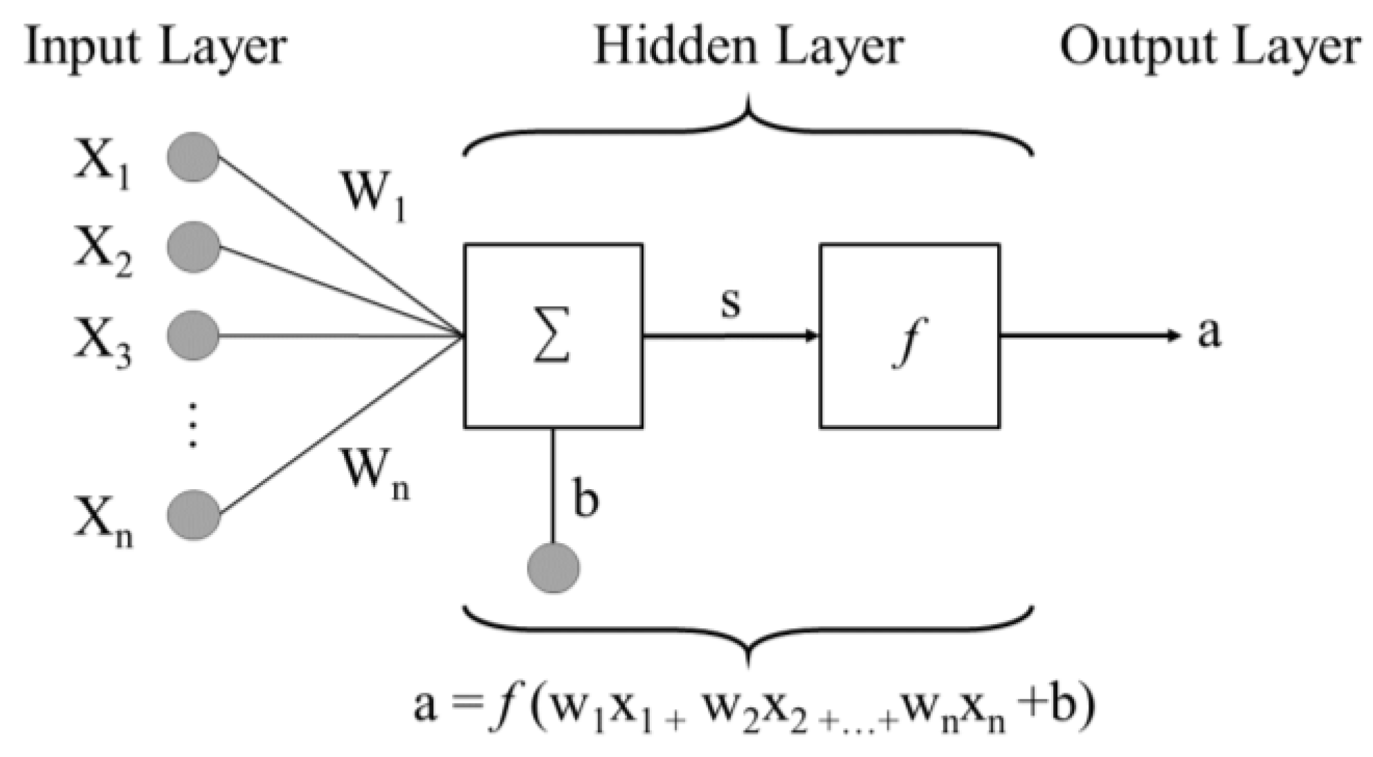
2.4.1. BP (Backpropagation)

During training, the sigmoid function was used as the transfer function from the input layer to the hidden layer and the linear function from the hidden layer to the output. The nonlinear damping least-squares (L-M) algorithm [34] was the training optimization method, and mapminmax normalized input/output data. The target error was 0.001, with a 0.001 learning rate and 50 maximum training steps. The optimal neural network topology was needed. The input layer consisted of seed-to-seed static friction coefficient (E), seed-to-steel-plate static friction coefficient (F), and seed-to-seed rolling friction coefficient (G), while the output was the seed resting angle. Based on Reference [35], the hidden layer had 7 nodes.

2.4.2. GA-BP (Genetic Algorithm–Backpropagation)

The GA-BP algorithm fully leverages the global search advantages of genetic algorithms. It optimizes the BP neural network structure and parameters by combining genetic algorithms. Genetic algorithms evolve individuals (BP network parameter sets) toward higher fitness through operations like selection, crossover, and mutation. In the GA-BP configuration, the population size was 100, the iteration count was 150, normGeomSelect was the function, the crossover coefficient was 0.8, and the mutation coefficient was 0.2.

2.4.3. PSO (Particle Swarm Optimization)

PSO maintains a set of candidate solutions (particles) that collaboratively search to find the global optimum. Each particle represents potential solutions with a fitness value. Based on its own and the best fitness among all particles, a particle adjusts its “flight” direction and speed toward the optimum. In the PSO algorithm, the learning rate was 0.6, the inertia factor was 0.1, the initial population was 50, and the acceleration factors c1 and c2 were both 2. The iteration count was 100.

2.4.4. SA (Simulated Annealing)

SA is a probabilistic optimization algorithm that achieves global optimization by accepting worse solutions with decreasing probability through random sampling. This enables escaping local optima to reach the global optimum. In the SA algorithm, the number of cycles was 100, the maximum iterations were 100, the upper and lower bounds were [0.647, 0.747, 0.447] and [0.513, 0.613, 0.313], respectively, and the Metropolis chain length L was 300.

2.4.5. Data Analysis and Processing

The algorithms were implemented in Matlab R2020b. Model predictive performance was evaluated using the coefficient of determination (R²), mean squared error (MSE), and mean absolute error (MAE). A larger R² indicates a higher model fit, while lower MSE and MAE indicate better accuracy and stability.

3. Results and Discussion

3.1. Simulation Calibration Test Results

The Plackett–Burman experiment results are presented in

Table 4. Plackett–Burman experiment design scheme and results.

No.	Test Parameters								Repose Angle θ (°)
	A	B	C	D	E	F	G	H
1	1	1	−1	1	1	−1	1	−1	23.62
2	−1	1	1	1	−1	1	1	−1	21.64
3	1	−1	1	1	1	1	−1	1	32.67
4	−1	1	−1	−1	1	1	1	1	39.59
5	−1	−1	1	1	−1	−1	1	1	18.78
6	−1	−1	−1	1	1	1	−1	−1	32.09
7	1	−1	−1	−1	−1	1	1	1	19.77
8	1	1	−1	1	−1	−1	−1	1	8.95
9	1	1	1	−1	−1	1	−1	−1	10.88
10	−1	1	1	−1	1	−1	−1	1	16.56
11	1	−1	1	−1	1	−1	1	−1	19.79
12	−1	−1	−1	−1	−1	−1	−1	−1	3.87
13	0	0	0	0	0	0	0	0	23.79

. A variance analysis identified significant simulation parameters, as shown in

Table 5. Plackett–Burman variation analysis.

Parameters	Degree of Freedom	Sum of Squares	F-Value	p-Value
A	1	23.66	3.06	0.1786
B	1	2.74	0.3537	0.5939
C	1	4.78	0.6173	0.4894
D	1	62.06	8.02	0.0661
E	1	539.08	69.68	0.0036 **
F	1	352.84	45.61	0.0066 **
G	1	121.41	15.69	0.0287 *
H	1	49.74	6.43	0.085

Note: ** in Table 5 indicates that the impact is extremely significant (p < 0.01), and * indicates that the impact is significant (p < 0.05).

. It can be observed from Table 5 that the seed-to-seed static friction coefficient and seed-to-steel-plate static friction coefficient have a p-value < 0.01, indicating a highly significant impact on the resting angle. The seed-to-seed rolling friction coefficient has a p-value < 0.05, indicating a significant impact. The remaining parameters have p-values > 0.05, indicating minimal impact.

The design and results of the steepest ascent experiment are presented in

Table 6. Steepest climbing test design scheme.

No.	Test Parameters			Repose Angle θ (°)	Relative Error Y (%)
	E	F	G
1	0.50	0.30	0.6	17.92	27.07%
2	0.54	0.34	0.64	22.93	6.67%
3	0.58	0.38	0.68	24.18	1.59%
4	0.62	0.42	0.72	25.73	4.51%
5	0.66	0.46	0.76	28.15	12.72%
6	0.70	0.50	0.8	36.26	32.24%

. As the seed-to-seed static friction coefficient, seed-to-seed rolling friction coefficient, and seed-to-steel-plate static friction coefficient increase, the simulated resting angle also increases. However, the relative error exhibits an initial decrease followed by an increase. The relative error is minimized in the third group, leading to the selection of the third group’s level as the center point for the Central Composite Design.

The design and results of the Central Composite Design experiment are presented in

Table 7. Central Composite Design experiment: design scheme and results.

No.	Test Parameters			Relative Error Y (%)
	E	F	G
1	−1	−1	−1	6.04
2	1	−1	−1	1.75
3	−1	1	−1	3.23
4	1	1	−1	0.53
5	−1	−1	1	6.47
6	1	−1	1	5.06
7	−1	1	1	4.68
8	1	1	1	5.29
9	−1.682	0	0	6.15
10	1.682	0	0	2.27
11	0	−1.682	0	5.69
12	0	1.682	0	2.03
13	0	0	−1.682	2.58
14	0	0	1.682	5.06
15	0	0	0	1.49
16	0	0	0	1.38
17	0	0	0	1.05
18	0	0	0	2.24
19	0	0	0	1.42
20	0	0	0	2.15
21	0	0	0	2.38
22	0	0	0	2.42
23	0	0	0	1.45

. The variance analysis results are shown in

Table 8. Variation analysis of Central Composite Design test’s quadratic model.

Source of Variance	Mean Square	Degree of Freedom	Sum of Squares	p-Value
Model	75.35	7	10.48	<0.0001 **
E	15.01	1	15.01	<0.0001 **
F	10.10	1	10.10	0.0002 **
G	14.60	1	14.60	<0.0001 **
EG	4.79	1	4.79	0.0035 **
E2	11.97	1	11.97	<0.0001 **
F2	8.80	1	8.80	0.0003 **
G2	8.47	1	8.47	0.0003 **
Residual	6.01	15	0.400 8
Lack-of-fit	3.88	7	0.554	0.1635
Pure Error	2.13	8	0.266 7
Cor Total	79.36	22

Note: ** in Table 8 indicates that the impact is extremely significant (p < 0.01).

. According to the analysis, the effects of E, F, G, EG, E², F², and G² on the relative resting-angle error are extremely significant. The effect of EF is significant, while that of FG is not significant. The fitted regression model has a p < 0.0001 significance, indicating a highly significant relationship between the resting angle and the equation. The lack-of-fit term has a p-value of 0.4234 > 0.05, suggesting good model fit without lack of fit. The coefficient of determination R² is 0.9544, and the adjusted R² is 0.9228, very close to 1. Together, these demonstrate the high significance of the regression model, its ability to reliably reflect the situation, and its suitability for subsequent resting angle prediction.

Figure 7a shows the interactive effects of the seed-to-seed rolling friction coefficient (F) and the seed-to-steel-plate static friction coefficient (G) on the evaluation indicator when the seed-to-seed static friction coefficient (E) is fixed. Figure 7b shows the effects of E and G when F is fixed. Figure 7c shows the effects of E and F when G is fixed. It can be observed that when E is fixed, G decreases monotonically for constant F. When G is fixed, F first decreases and then increases. Although the relative error under two-factor interaction showed some patterns, the relationship could not be easily described by simple linear models. Therefore, machine learning regression models were considered for optimized fitting.

3.2. Machine Learning Regression Models

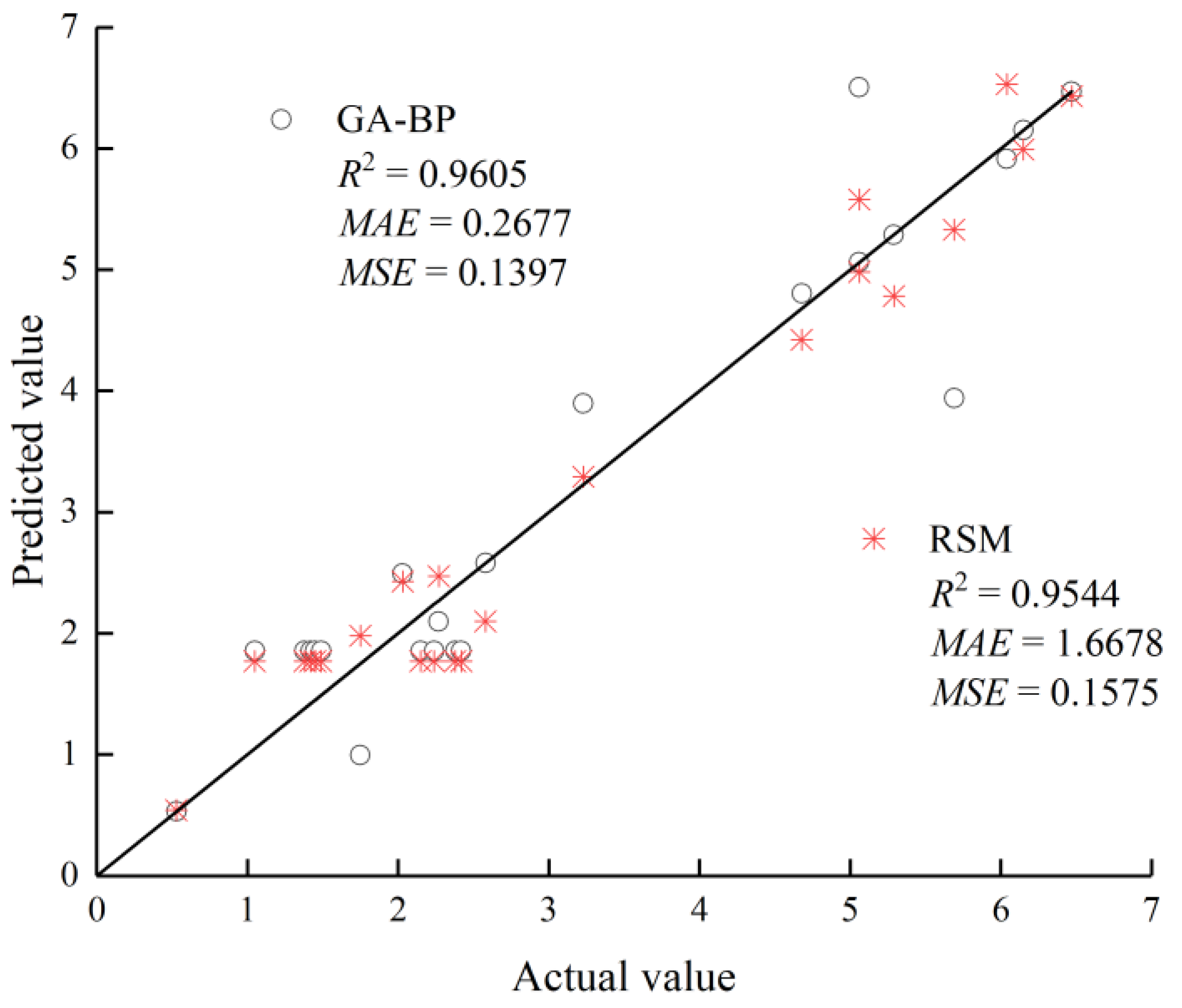
3.2.1. Model Comparison

Four algorithms performed regression modeling on the data. The models were compared based on R², MSE, and MAE values to determine the most suitable model for red clover seed calibration.

Table 9. Model comparison.

Arithmetic	R2	MSE	MAE
BP	0.9017	0.3850	0.3271
GA-BP	0.9605	0.1397	0.2677
PSO	0.9572	0.1479	0.2973
SA	0.99	0.1975	0.4704

shows the comparative results across multiple repetitions using the four algorithms.

Table 9 shows that R²’s ranks are SA > GA-BP > PSO > BP for the four models. SA is a stochastic search algorithm, GA-BP combines genetic algorithms with BP neural networks, PSO is particle swarm optimization, and BP is traditional backpropagation. Considering the search strategies, SA and PSO have stronger global search capabilities, GA-BP combines GA’s global search with BP’s local search, and BP relies on local search. This could explain why SA and GA-BP outperform PSO and BP in fitting. However, determining absolute superiority based solely on R² is difficult. A comprehensive MSE and MAE analysis is needed. MSE’s ranks are GA-BP < PSO < SA < BP, while MAE’s ranks are GA-BP < PSO < BP < SA. MSE reflects precision, and MAE reflects stability. GA-BP outperforms in both, indicating a model combining accuracy and stability. The combination of genetic algorithms and BP neural networks in GA-BP likely explains its overall better performance in global and local searches.

Figure 8 compares the measured and predicted values obtained from the GA-BP and RSM models. The GA-BP model demonstrated better performance in terms of accuracy, stability, and goodness of fit (R² = 0.9605, MSE = 0.1397, MAE = 0.2677) compared to RSM (R² = 0.9544, MSE = 0.1575, MAE = 1.6678). This indicates that the GA-BP model achieved superior fitting results for this study, constructing a higher precision model with fewer errors, consistent with the findings of Bu (2021) and Nanvakenari (2021) [36,37].

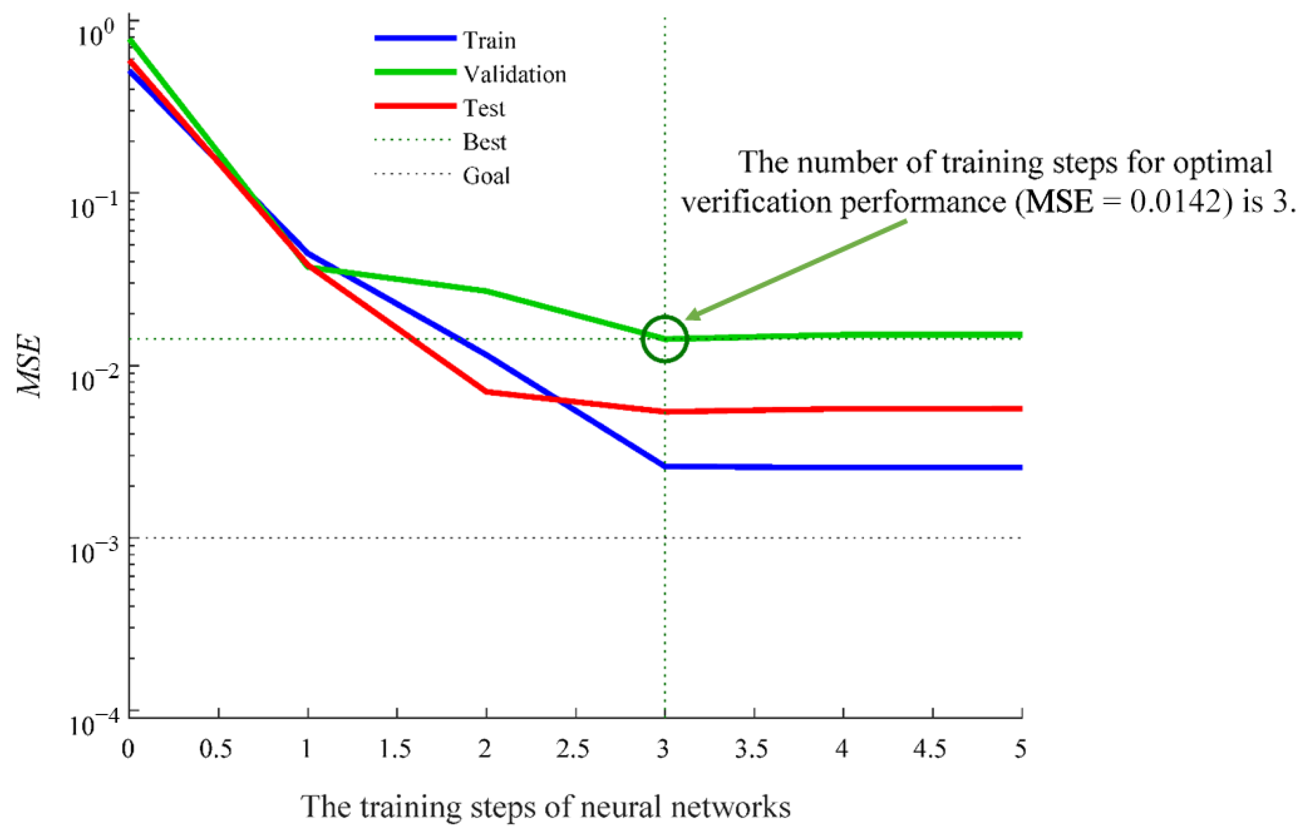
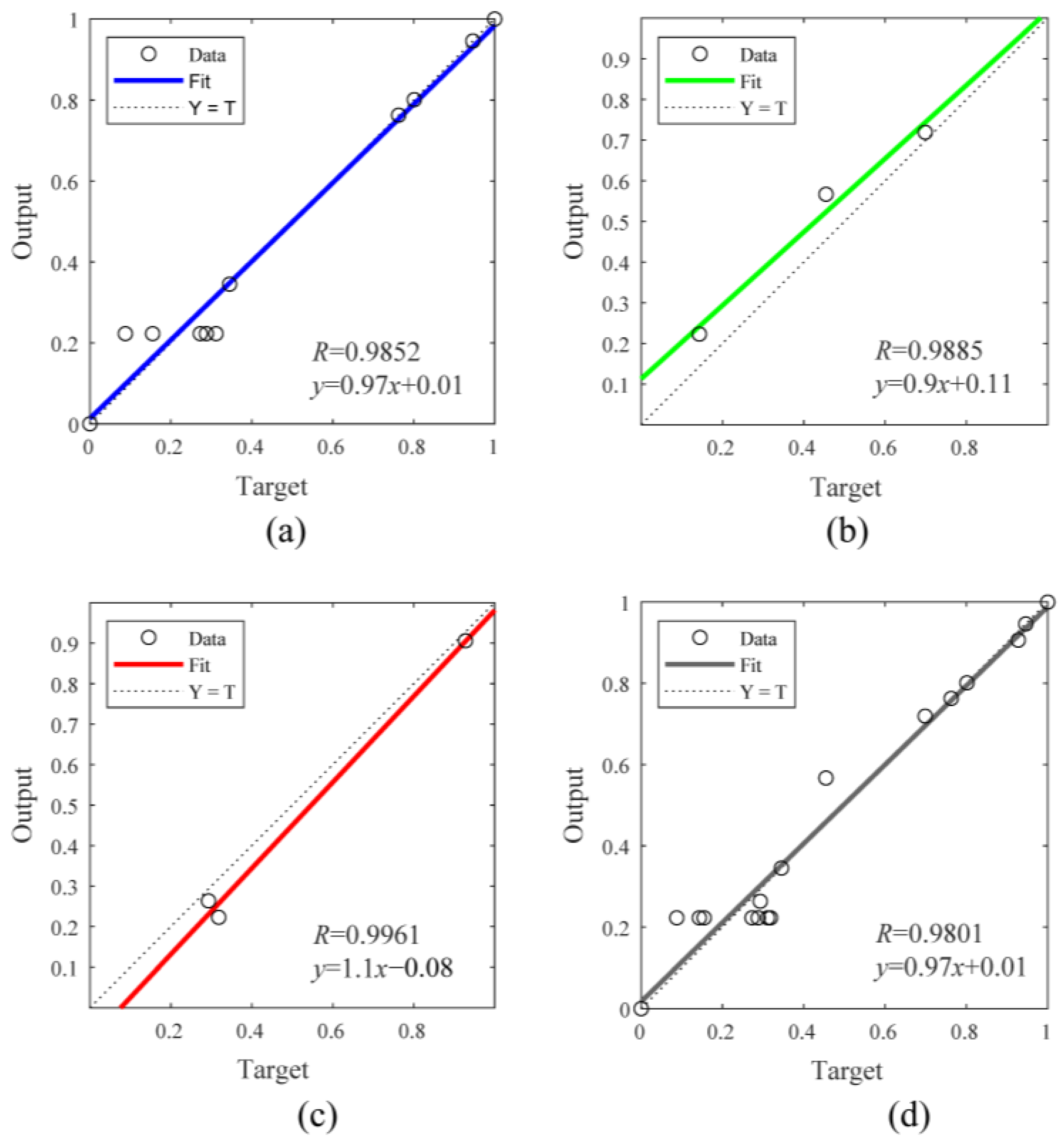
3.2.2. Model Evaluation

For the selected GA-BP model, the performance evaluation was conducted based on the model’s MSE, as shown in Figure 9. The figure illustrates that the model’s MSE shows a decreasing trend during the training process, indicating a more accurate fit to the training data as the training advances. Optimal performance is attained at the third training step, suggesting that the neural network training is nearing completion at this stage. This highlights the rapid and stable convergence of the GA-BP model during training, rendering it highly suitable for experimental applications.

The training, validation, and testing performance of the GA-BP model analyzed in this study are depicted in Figure 10. From the graph, it is evident that the correlation coefficients for the training, validation, testing, and combined datasets are 0.9852, 0.9885, 0.9961, and 0.9801 for the training, validation, testing, and combined datasets, respectively. These coefficients indicate the robust fitting effect of the model and commendable generalization ability. The closely aligned correlation coefficients across the datasets suggest the absence of significant overfitting or underfitting. The GA-BP model exhibits strong performance in this study, demonstrating high precision and robust generalization ability. Consequently, this model holds promise for application in subsequent experimental research.

3.2.3. GA-BP Optimization Experiment

The GA-BP model exhibited remarkable fitting accuracy. Through iterative cycles, the search halted at 150 evolutionary iterations when the optimum was reached. The individual with fitness closest to the optimum was selected. The final optimized results were a static friction coefficient of 0.618 for seed–seed and 0.395 for seed–steel plate and a rolling friction coefficient of 0.652 for seed–seed. Using the GA-BP optimized parameters, the simulated angle of repose for red clover seeds was 24.33°, with a 0.98% error compared to the physical experiments. The established red clover seed model and parameters hold potential for application in subsequent discrete element simulations.

3.3. Analysis of Test Results

Compared to the traditional discrete element calibration method using RSM analysis for parameter optimization, the GA-BP model is used for data analysis and processing, which requires a lot of iterative calculations but can more accurately solve the nonlinear relationship between variables, which is beneficial for the accuracy of discrete element simulation calibration. From the theoretical basis of the two models, the RSM experimental analysis method establishes an effective prediction model through different experiments, while GA-BP focuses on analyzing the data, which makes it easier to explore the data relationships compared to designing an experimental system [38]. In application areas, scholars have used neural network models combined with RSM analysis for data analysis, but there is no related research on processing the large number of complex data in the discrete element simulation calibration process [18,39]. This study compares different neural network machine learning models with RSM analysis methods and explores the feasibility of using the GA-BP model to analyze the experimental results of red clover seed discrete element calibration. The experimental results are consistent with those of Ding et al., indicating that neural network methods can be used in the field of seed discrete element calibration to improve simulation accuracy [40]. This method can provide a reference for the calibration of related discrete element simulation parameters.

4. Conclusions

(1) Physical experiments determined the fundamental properties of red clover seeds. The collision restitution coefficient range, static friction coefficient range, and rolling friction coefficient range between seeds were obtained using a high-speed camera system and an inclined plane instrument. The values ranged from 0.4 to 0.6, 0.5 to 0.7, and 0.6 to 0.9, respectively. The ranges between the seeds and the steel plates were 0.5 to 0.7, 0.3 to 0.5, and 0.2 to 0.5, respectively.

(2) Using the physically determined parameters to select simulation parameters, the Plackett–Burman experiment identified the parameters significantly affecting the repose angle. The steepest ascent experiment then determined the optimal range of the significant parameters. Finally, the Central Composite Design experiment was conducted using the optimal parameter combination.

(3) A comparative analysis of the BP, GA-BP, PSO, and SA models based on R², MAE, and MSE revealed that GA-BP had the lowest MAE and MSE values, indicating the best accuracy and stability. Its R² was slightly lower than that of SA. Considering all factors, the GA-BP model was chosen to predict the repose angle of red clover seeds.

(4) A comparison of the R², MAE, and MSE of the GA-BP and RSM models shows that GA-BP performs well in terms of accuracy, stability, and goodness of fit. The validation of the predicted values demonstrates that GA-BP can be used for parameter optimization when calibrating red clover seed parameters.

References

1. Li, Y.; Wan, L.; Xu, Z.; Zhao, H.; Chen, H.; Song, J. Design of Automatic Control System for Plot Batch Seed Cleaning Machine. Nongye Gongcheng Xuebao/Trans. Chin. Soc. Agric. Eng. 2021, 37, 23–33. [Google Scholar] [CrossRef]
2. Ma, X.; Liu, M.; Hou, Z.; Gao, X.; Bai, Y.; Guo, M. Numerical Simulation and Experimental Study on the Pelletized Coating of Small Grain Forage Seeds. Nongye Gongcheng Xuebao/Trans. Chin. Soc. Agric. Eng. 2023, 39, 43–52. [Google Scholar] [CrossRef]
3. Zhao, X.; Zhang, T.; Liu, F.; Li, N.; Li, J. Sunflower Seed Suction Stability Regulation and Seeding Performance Experiments. Agronomy 2023, 13, 54. [Google Scholar] [CrossRef]
4. Li, X.; Liu, Y.; An, F.; Wang, H.; Xu, Y. Flow Field Distribution and Morphology Variation of Particles in Planetary Ball Milling. Binggong Xuebao/Acta Armamentarii 2022, 43, 876–891. [Google Scholar] [CrossRef]
5. Hou, Z.; Dai, N.; Chen, Z.; Qiu, Y.; Zhang, X. Measurement and Calibration of Physical Property Parameters for Agropyron Seeds in a Discrete Element Simulation. Nongye Gongcheng Xuebao/Trans. Chin. Soc. Agric. Eng. 2020, 36, 46–54. [Google Scholar] [CrossRef]
6. Wang, S.; Yu, Z.; Aorigele; Zhang, W. Study on the Modeling Method of Sunflower Seed Particles Based on the Discrete Element Method. Comput. Electron Agric. 2022, 198, 107012. [Google Scholar] [CrossRef]
7. Bembenek, M.; Buczak, M.; Baiul, K. Modelling of the Fine-Grained Materials Briquetting Process in a Roller Press with the Discrete Element Method. Materials 2022, 15, 4901. [Google Scholar] [CrossRef]
8. Hao, B.; Tong, X.; Chen, Z.; Liu, H. Calibration of Simulation Parameters for Wind Erosion Gas-Solid Two-Phase Flow in Arid and Semiarid Soils. Rev. Bras. Eng. Agric. Ambient. 2022, 26, 564–570. [Google Scholar] [CrossRef]
9. Liu, M.; Hou, Z.; Ma, X.; Zhang, X.; Dai, N. Determination and Testing of Pelletized Coated Particles. INMATEH Agric. Eng. 2022, 66, 247–256. [Google Scholar] [CrossRef]
10. Adilet, S.; Zhao, J.; Sayakhat, N.; Chen, J.; Nikolay, Z.; Bu, L.; Sugirbayeva, Z.; Hu, G.; Marat, M.; Wang, Z. Calibration Strategy to Determine the Interaction Properties of Fertilizer Particles Using Two Laboratory Tests and DEM. Agriculture 2021, 11, 592. [Google Scholar] [CrossRef]
11. Chen, Z.; Wang, G.; Xue, D. An Approach to Calibration of BPM Bonding Parameters for Iron Ore. Powder Technol. 2021, 381, 245–254. [Google Scholar] [CrossRef]
12. Zhang, Z.; Mei, F.; Xiao, P.; Zhao, W.; Zhu, X. Discrete Element Modelling and Simulation Parameters Calibration for the Compacted Straw Cube. Biosyst. Eng. 2023, 230, 301–312. [Google Scholar] [CrossRef]
13. Cui, Z. Research on Optimization of Adaptive Path Planning for 3D Printing. Master’s Thesis, Dalian University of Technology, Dalian, China, 2022. [Google Scholar] [CrossRef]
14. Agatonovic-Kustrin, S.; Zecevic, M.; Zivanovic, L.; Tucker, I.G. Application of Artificial Neural Networks in HPLC Method Development. J. Pharm. Biomed. Anal. 1998, 17, 69–76. [Google Scholar] [CrossRef] [PubMed]
15. Veza, I.; Spraggon, M.; Fattah, I.M.R.; Idris, M. Response Surface Methodology (RSM) for Optimizing Engine Performance and Emissions Fueled with Biofuel: Review of RSM for Sustainability Energy Transition. Results Eng. 2023, 18, 101213. [Google Scholar] [CrossRef]
16. Bourquin, J.; Schmidli, H.; van Hoogevest, P.; Leuenberger, H. Advantages of Artificial Neural Networks (ANNs) as Alternative Modelling Technique for Data Sets Showing Non-Linear Relationships Using Data from a Galenical Study on a Solid Dosage Form. Eur. J. Pharm. Sci. 1998, 7, 5–16. [Google Scholar] [CrossRef] [PubMed]
17. Hammoudi, A.; Moussaceb, K.; Belebchouche, C.; Dahmoune, F. Comparison of Artificial Neural Network (ANN) and Response Surface Methodology (RSM) Prediction in Compressive Strength of Recycled Concrete Aggregates. Constr. Build. Mater. 2019, 209, 425–436. [Google Scholar] [CrossRef]
18. Tang, X.; Yue, Y.; Shen, Y. Prediction of Separation Efficiency in Gas Cyclones Based on RSM and GA-BP: Effect of Geometry Designs. Powder Technol. 2023, 416, 118185. [Google Scholar] [CrossRef]
19. Liang, F.; Sun, L.; Zeng, Z.; Kang, J. Treatment of Surfactant Wastewater by Foam Separation: Combining the RSM Method and WOA-BP Neural Network to Explore Optimal Process Conditions. Chem. Eng. Res. Des. 2023, 193, 85–98. [Google Scholar] [CrossRef]
20. Fetimi, A.; Dâas, A.; Benguerba, Y.; Merouani, S.; Hamachi, M.; Kebiche-Senhadji, O.; Hamdaoui, O. Optimization and Prediction of Safranin-O Cationic Dye Removal from Aqueous Solution by Emulsion Liquid Membrane (ELM) Using Artificial Neural Network-Particle Swarm Optimization (ANN-PSO) Hybrid Model and Response Surface Methodology (RSM). J. Environ. Chem. Eng. 2021, 9, 105837. [Google Scholar] [CrossRef]
21. Dai, N.; Hou, Z.; Qiu, Y.; Zhang, X. Calibration and Experiment of Discrete Element Simulation Parametersof Red Clover Seeds. J. Hebei Agric. Univ. 2021, 44, 92–98. [Google Scholar] [CrossRef]
22. Zhou, L.; Dong, Q.; Yu, J.; Wang, Y.; Chen, Y.; Li, M.; Wang, W.; Yu, Y.; Yuan, J. Validation and Calibration of Maize Seed&ndash;Soil Inter-Parameters Based on the Discrete Element Method. Agronomy 2023, 13, 2115. [Google Scholar] [CrossRef]
23. Zhang, R.; Jiao, W.; Zhou, J.; Qi, B.; Liu, H.; Xia, Q. Parameter Calibration and Experiment of Rice Seeds Discrete Element Model Witrdifferent Filling Particle Radius. Trans. Chin. Soc. Agric. Mach. 2020, 51, 227–235. [Google Scholar] [CrossRef]
24. Liu, M.; Hou, Z.; Ma, X.; Dai, N.; Zhang, X. Simulation Parameter Calibration and Experiment of Purple Flower Head Seed Based on Discrete Element. Jiangsu Agric. Sci. 2022, 50, 168–175. [Google Scholar] [CrossRef]
25. Chen, L.; Sun, Y.H.; Xie, G.P.; Mao, Q. Analysis of Chewing Process Based on the Discrete Element Method. J. Jilin Univ. 2014, 44. [Google Scholar] [CrossRef]
26. Peng, C.; Zhou, T.; Song, S.; Fang, Q.; Zhu, H.; Sun, S. Measurement and Analysis of Restitution Coeffcient of Black Soldier Fly Larvaein Collision Models Baseo on Hertz Contact Theory. Trans. Chin. Soc. Agric. Mach. 2021, 52, 125–134. [Google Scholar] [CrossRef]
27. Zeng, Z.; Ma, X.; Cao, X.; Li, Z.; Wang, X. Critical Review of Applications of Discrete Element Method in Agricultural Engineering. Trans. Chin. Soc. Agric. Mach. 2021, 52, 1–20. [Google Scholar] [CrossRef]
28. Lenaerts, B.; Aertsen, T.; Tijskens, E.; De Ketelaere, B.; Ramon, H.; De Baerdemaeker, J.; Saeys, W. Simulation of Grain–Straw Separation by Discrete Element Modeling with Bendable Straw Particles. Comput. Electron. Agric. 2014, 101, 24–33. [Google Scholar] [CrossRef]
29. Hou, J.; Xie, F.; Wang, X.; Liu, D.; Chen, Z. Measurement of Contact Physical Parameters of Flexible RiceStraw and Discrete Element Simulation Calibration. Acta Agric. Univ. Jiangxiensis 2022, 44, 747–758. [Google Scholar] [CrossRef]
30. Coetzee, C.J.; Els, D.N.J.; Dymond, G.F. Discrete Element Parameter Calibration and the Modelling of Dragline Bucket Filling. J. Terramech. 2010, 47, 33–44. [Google Scholar] [CrossRef]
31. Yang, L.; Wang, F. Calibration of Parameters of Coated Carrot Seeds Required in DiscreteElement Method Simulation Based on Repose Angle of Particle Heap. J. Agric. Mech. Res. 2023, 45, 143–150. [Google Scholar] [CrossRef]
32. Xu, X.; Wei, H.; Yan, J.; Bao, G.; Du, Y. Parameter Calibration of Peanut Pods Discrete Element Simulation. J. Chin. Agric. Mech. 2022, 43, 81–89. [Google Scholar] [CrossRef]
33. Kumar, R.; Patel, C.M.; Jana, A.K.; Gopireddy, S.R. Prediction of Hopper Discharge Rate Using Combined Discrete Element Method and Artificial Neural Network. Adv. Powder Technol. 2018, 29, 2822–2834. [Google Scholar] [CrossRef]
34. Gai, L. Exploration of Manufacturing Technique and Mechanical Performance Prediction of Reconsolidated Square Materials of Cotton Stalk. Master’s Thesis, Northwest Agriculture and Forestry University, Xianyang, China, 2014. [Google Scholar]
35. Zhang, H.; Ma, Y.; Li, Y.; Zhang, R.; Zhang, X. Rupture Energy Prediction Model for Walnut Shell Breaking Based on Genetic BP Neural Network. Nongye Gongcheng Xuebao/Trans. Chin. Soc. Agric. Eng. 2014, 31, 78–84. [Google Scholar] [CrossRef]
36. Bu, X.; Xu, Y.; Zhao, M.; Li, D.; Zou, J.; Wang, L.; Bai, J.; Yang, Y. Simultaneous Extraction of Polysaccharides and Polyphenols from Blackcurrant Fruits: Comparison between Response Surface Methodology and Artificial Neural Networks. Ind. Crops Prod. 2021, 170, 113682. [Google Scholar] [CrossRef]
37. Nanvakenari, S.; Movagharnejad, K.; Latifi, A. Evaluating the Fluidized-Bed Drying of Rice Using Response Surface Methodology and Artificial Neural Network. LWT 2021, 147, 111589. [Google Scholar] [CrossRef]
38. Sabour, M.R.; Amiri, A. Comparative Study of ANN and RSM for Simultaneous Optimization of Multiple Targets in Fenton Treatment of Landfill Leachate. Waste Manag. 2017, 65, 54–62. [Google Scholar] [CrossRef]
39. Li, J.; Yao, X.; Xu, K. A Comprehensive Model Integrating BP Neural Network and RSM for the Prediction and Optimization of Syngas Quality. Biomass Bioenergy 2021, 155, 106278. [Google Scholar] [CrossRef]
40. Ding, X.; Li, K.; Hao, W.; Yang, Q.; Yan, F.; Cui, Y. Calibration of Simulation Parameters of Camellia Oleifera SeedsBased on RSM and GA-BP-GA Optimization. Nongye Jixie Xuebao/Trans. Chin. Soc. Agric. Mach. 2023, 54, 139–150. [Google Scholar] [CrossRef]
Figure 1. Compression and shear test of red clover seed.
Agronomy 13 02670 g001
Figure 2. Crash Recovery Coefficient Test: (a) seed board; (b) seed rebound process; (c) high-speed camera.
Agronomy 13 02670 g002
Figure 3. Friction Coefficient Test: (a) CNY-1 inclinometer; (b) analysis of forces on an inclined object.
Agronomy 13 02670 g003
Figure 4. Measurement of the physical angle of repose.
Agronomy 13 02670 g004
Figure 5. Discrete element model of red clover seeds: (a) seed geometric modeling; (b) seed simulation modeling.
Agronomy 13 02670 g005
Figure 6. Typical structure of a neuron.
Agronomy 13 02670 g006
Figure 7. Effects of interactive factors on the evaluation indicator: (a) E fixed; (b) F fixed; (c) G fixed.
Agronomy 13 02670 g007
Figure 8. Measured versus predicted values.
Agronomy 13 02670 g008
Figure 9. Evaluation of MSE model performance.
Agronomy 13 02670 g009
Figure 10. Regression analysis: (a) training; (b) validation; (c) test; (d) all.
Agronomy 13 02670 g010