Estimating Chlorophyll Content, Production, and Quality of Sugar Beet under Various Nitrogen Levels Using Machine Learning Models and Novel Spectral Indices

Abstract

Accurately estimating crop performance under various fertilizer levels in a rapid and non-destructive manner has become a vital aspect of precision agriculture technology for both economic and environmental benefits. This study aimed to estimate different sugar beet parameters, such as total chlorophyll (Chlt), chlorophyll a (Chla), chlorophyll b (Chlb), root yield (RY), sugar yield (SY), and sugar content (SC) under five nitrogen (N) levels (0, 30, 60, 90, and 120 kg N ha⁻¹). This was achieved by using a combination of the gradient boosting regression (GBR) model with published and newly developed two- and three-band spectral indices (2D- and 3D-SRIs). The results showed that the N levels had the highest proportion of variations (80.4–92.9%) for all parameters, except for SC, which had more variation (59.9%) according to year than the N levels (37.2%). All parameters, except SC, showed a significant increase with gradually increasing N levels. Additionally, the N levels displayed linear and strong positive relationships with the chlorophyll parameters, and linear and strong negative relationships with SC, while these relationships were quadratic and strong with RY and SY. Several published and novel 3D-SRIs exhibited moderate to strong relationships (R² = 0.65–0.89) with all parameters. The newly developed 3D-SRIs, which involve wavelengths from the visible, near-infrared, and red-edge regions, such as NDI_{536, 538, 534}, NDI_{738, 750, 542}, and NDI_{448, 734, 398}, were effective in accurately estimating all parameters. Combining 2D-SRIs, 3D-SRIs, and the aggregate of all spectral indices (ASRIs) with GBR models could be a robust strategy for estimating the six observed parameters with reasonable precision. The GBR-ASF-6 SRIs and the GBR-ASF-7 SRIs models performed better in predicting Chl content and SC with R² values of 0.99 and 0.99 (RMSE = 0.073 and 1.568) for the training dataset and R² values of 0.65 and 0.78 (RMSE = 0.354 and 6.294) for the testing datasets, respectively. The obtained results concluded that published and newly developed 3D-SRIs, GBR based on 2D-SRIs or 3D-SRIs, and the aggregate of all ASRIs can be used in practice to accurately estimate the Chl content, production, and quality of sugar beet across a wide range of N levels under semiarid conditions.

1. Introduction

Sugar beet (Beta vulgaris L.) is the second most important sugar crop worldwide, following sugarcane, in terms of sucrose production. It contributes to roughly 20% of the world’s total sugar production and has a higher sucrose content (13–20%) compared to sugarcane. It is a biennial crop and a member of the Chenopodiaceae family. It also forms storage roots during the spring and autumn of the first year of its vegetative development stage under Mediterranean climatic conditions [1]. Sugar beet is a crop that has a significant correlation with fertilizer management [2]. The growth, yield of roots, sugar, and quality of this crop are reliant on nutrient levels [2,3]. Therefore, it is vital to carefully consider this factor when cultivating sugar beet [2,3,4]. Among all nutrients, nitrogen (N) is the most important, as it directly affects both the production and quality of sugar beet [5,6,7,8,9]. In order to achieve a balance between maximizing root yield (RY) and obtaining high-quality sugar, it is important to optimize N inputs in the production systems of sugar beet. This is because insufficient or excessive amounts of N can seriously affect the growth, production, and sugar quality of this crop [10,11,12,13,14]. Insufficient N application leads to smaller leaves and pale green foliage, lower chlorophyll content, stunted leaf growth, and decreased root yield. It also diminishes the amount of solar radiation absorbed and accelerates leaf aging, ultimately resulting in a significant decrease in RY [5,15,16,17]. Conversely, applying too much N may lead to a prolonged plant cycle and delayed harvest time. Additionally, it may lead to an over-production of dark green leaves and excessive vegetative growth [14,16,17]. Moreover, it inhibits the translocation of photosynthetic assimilates from the aboveground parts to the tuber, which then reduces the concentrations and purity percentage of the sugar [18,19]. The unreasonable application of N is costly and causes serious environmental pollution. In general, sugar beets require 0.04 g N per cm⁻² of leaf to maintain a good balance between RY and sugar content (SC). This balance can be achieved by supplying 20 kg N ha⁻¹ [5]. Jaggard et al. [20] reported that an amount of 100–110 kg N ha⁻¹ is efficient to achieve a balance between the value of sugar beet and fertilizer prices in England. Koch et al. [21] found that an optimal N rate of 100–125 kg N ha⁻¹ is required to accomplish the maximum RY in Germany. However, in Greece, the optimal N rate can reach up to 252.5 kg N ha⁻¹ [22]. Mekdad and Rady [23] mentioned that the application of 350 kg N ha⁻¹ was more efficient than 200 kg N ha⁻¹ for enhancing all traits related to sugar beet roots, except for purity percentage and harvest index, under Egyptian conditions. It is obvious that sugar beet plants require optimal N levels in order to achieve a balance between root production, quality, and fertilizer prices. In this regard, there is an urgent need to develop an efficient method to monitor the N status of sugar beets in real time during the growing season. This will enhance both their production and quality while protecting the environment from N-pollution.

Generally, the chlorophyll (Chl) content in the leaves is a crucial indicator of a plant’s health status. Pigment concentration, which can serve as a measure of both photosynthetic capacity and crop productivity [24], is strongly related to the N status of the plant [18]. Chlorophyll affects the utilization of light energy in agricultural photosynthesis, as well as the carbon budget and net primary production [25]. Because the Chl content is affected by the N status of plants, there is always a strong link between the Chl and N contents in plant leaves [26]. As a result, the Chl content in the leaves is considered a potential bio-indicator for monitoring crop growth and development as well as determining the nitrogen nutritional status of the crop [27]. A high N application rate increases the Chl concentration in the leaves, whereas low levels of N in the leaves result in pale green foliage due to a low Chl concentration [28]. This reflects that leaf Chl content and plant N status are strongly related. Therefore, plant N status can be determined using Chl monitoring techniques.

The SPAD-502 Chl meter has been successfully used in several crops to indirectly assess the amount of N in plant leaves. This is achieved in a rapid and non-destructive manner by monitoring the status of Chl of plant leaves. However, unfortunately, the SPAD meter reflects the Chl status of the entire plant canopy based on measurements of the Chl at the leaf scale, ignoring the vertical variation in leaf Chl content within the plant canopy. Therefore, the SPAD meter is not accurate for reflecting the Chl status of the entire plant canopy [29,30,31,32]. Consequently, there is a necessity for a fast, non-destructive, and cost-efficient alternative tool to accurately assess the status of Chl throughout the entire canopy. This tool would be essential for effectively monitoring and diagnosing the N nutritional status of crops, as well as regulating its use in sugar beets.

Hyperspectral technology has recently been developed due to advancements in remote sensing technology. It aims to address the limitations of the traditional methods used to measure plant traits such as Chl content, yield, and quality. These traditional methods are often laborious, invasive, and time-consuming for acquiring information about various plant traits [33,34,35,36,37,38,39]. The proximal remote sensing technique is capable of detecting the canopy spectral reflection at distances of less than 100 cm from the plant canopy in the range of visible (VIS) to shortwave infrared (SWIR) on the electromagnetic spectrum, making it more efficient for monitoring rapid and non-destructive changes in various vegetative and biochemical characteristics of plants [40,41,42,43,44]. The reflected radiation measurements are used to spectrally sense the crop canopy. When assessing crop canopies, the primary focus is electromagnetic radiation in the VIS (400–700 nm) and near-infrared (NIR, 700–1100 nm) spectral ranges. While the chlorophyll content of the leaves is determined in the VIS region, the interior structure of the mesophyll cells is determined in the NIR region [41,42,45,46].

Several studies have revealed the importance of selecting effective spectral reflectance indices (SRIs) and the most sensitive wavebands for estimating various biochemical and biophysical plant characteristics [47,48,49,50,51]. The canopy reflectance collected using hyperspectral remote sensing reflects all vegetation information. Therefore, it is important to develop new universal SRIs to optimize the existing ones and determine the best wavebands to accurately estimate plant characteristics at the canopy scale.

The various SRIs, which are derived from the ratios of canopy spectral reflectance at two or more wavelengths, are strongly associated with different plant characteristics and physiological functions, such as plant biomass, Chl and nitrogen contents, and water status. The interaction between VIS and NIR is useful for estimating N status. Amirruddin et al. [47] and Dray Jr et al. [52] discovered that the relative Chl content can be determined by measuring the absorbance of two separate wavelength areas (650 nm and 940 nm) in a leaf. This data can be used to build a dimensionless Chl content value, indicating the relative quantity of chlorophyll contained in the leaf. Additionally, because the green peak (550 nm) and red edge (660–770 nm) spectral ranges provide accurate information on crop growth, a number of SRIs have been established based on chosen wavelengths at these spectral regions for forecasting plant biophysical parameters such as leaf area index, plant biomass, and Chl content [48,49,50]. Precision agriculture and vegetation monitoring are used to calculate the NDVI as it is closely related to variations in Chl content and crop growth status [53,54]. Ray et al. [55] reported that the best wavelengths for assessing the plant N status of potato varieties were 520, 560, 660, 690, 730, 760, 780, 790, and 800 nm under different N and irrigation levels.

Although many SRIs may be calculated easily and have great potential to analyze and predict plant traits, these indices are often generated based on only two to three wavelengths. As a result, SRIs are less effective in estimating plant attributes under diverse growth conditions and are more sensitive to the different factors influencing canopy spectral signatures such agronomic treatments, phenological growth stages, cultivars, seasons, and climatic conditions [37,56,57,58]. Additionally, while there are hundreds of SRIs available, just a small number of SRIs are used in published work. Furthermore, the regression analyses used for assessing the relationship between spectral reflectance and plant attributes are based on only one SRI. Therefore, there are strong arguments in favor of combining multiple different SRIs into a single index when estimating plant features in order to enhance the prediction analysis and modeling of plant attributes using machine learning.

Gradient boosting regression (GBR) is a machine learning model that has experienced a notable surge in the development and utilization of computing resources and intelligence across various academic disciplines in recent years. High-value characteristics for discrimination and prediction can, for instance, be identified using model-based feature selection techniques [59]. This approach can enhance model performance by limiting over-fitting and removing unused features. Keeping the original feature representation has the added benefit of improving interpretability [60]. Algorithms for feature selection are increasingly needed for modeling and prediction [61]. Numerous studies have been conducted to examine the use of several techniques in reducing the dimensionality of data, including GBR, random forest (RF), and decision tree (DT). Based on the RF model, all variables are ranked according to relevance [62]. A back-propagation neural network index was developed by Glorfeld [63] to determine the most crucial factors. Hyperparameter selection, which offers a variety of benefits, also has a considerable impact on the performance of any machine learning model. For instance, it might enhance the effectiveness of machine learning algorithms [64] and the fairness and repeatability of scientific studies [65]. Given that it directly influences how training algorithms behave, it could be extremely important in improving the prediction model [66].

To date, there have been a few studies that have directly compared the ability of 3D-SRIs to assess sugar beet attributes in nitrogen management techniques. Thus, the primary purpose of this study was to assess the possibility to create robust 2D- and 3D-SRIs to estimate the production and quality of sugar beet across different N levels.

The specific objectives of the current study were to (i) examine the effects of different nitrogen levels on several characteristics of sugar beet, such as Chlt, Chla, Chlb, RY, SY, and SC; (ii) create multiple 2D and 3D-SRIs from the spectral reflectance of a sugar beet canopy and evaluate their performance to quantify various characteristics of sugar beet; and (iii) evaluate the performance of the GBR model and data fusion based on common and 3D-SRIs, to forecast the characteristics of sugar beet under different N levels.

2. Materials and Methods

2.1. Experimental Site and Experimental Design

The Multigerm sugar beet cultivar DSA007 (Lilly) imported from Denmark by the Egyptian Ministry of Agriculture was used as the plant material in this study. The seeds of the sugar beet cultivar were planted on September 25th during two successive growing seasons (2020/2021 and 2021/2022) under a drip irrigation system at a farmland in Al Nubaria District, El-Behaira Governorate (N 30°40′59.88″, E 30°9′11.52″), Egypt. The major soil texture of the experimental site is sand loam (8.5% coarse sand, 77.5% fine sand, 8.8% silt, and 5.2% clay) with a bulk density of 1.69 g cm⁻³, electrical conductivity of 2.6 dS m⁻¹, field capacity of 14.0%, wilting point of 6.0%, and an accessible water content of 8.5%.

A randomized block design was used with five repetitions to arrange the five fertigation amounts of applied nitrogen (0, 30, 60, 90, and 120 kg N ha⁻¹). The nitrogen (N) was applied in two equal doses as ammonium nitrate (33.5% N). The first dose was applied during the first irrigation, and the second dose was applied during the second irrigation. The appropriate amounts of phosphorus (calcium superphosphate, 15.5% P₂O₅) and potassium (potassium sulfate, 48% K₂O) fertilizers were applied during seedbed preparation. The rate of application was 200 kg ha⁻¹ for phosphorus and 100 kg ha⁻¹ for potassium. A Venturi fertilizer injector was used to mix the fertilizer into the drip irrigation system. All recommended agronomic and plant protection practices were diligently followed, from the planting stage to harvesting, in accordance with Leilah and Khan [7]. The area of each plot was 35.2 m², with dimensions 3.6 m wide and 7 m long. Additionally, each plot was irrigated using a drip irrigation system. Each plot consisted of six polyethylene lateral lines (16 mm) spaced 0.6 m apart, with built-in drippers delivering 4 L h⁻¹ and spaced 0.25 m apart. Drippers had a circular wetting pattern with an approximate diameter of 30 cm. To prevent any interference between different treatments, data were mainly collected from the central rows, even with a buffer area separating the various experimental plots. The amount of irrigation water applied was determined based on reference evapotranspiration ($E{T}_O$) using data from Class A pan evaporation. The formula by Doorenbos and Kassam [67] was used to compute the reference evapotranspiration ($E{T}_O$ mm day⁻¹) according to the Class A pan evaporation method as follows:

$$E{T}_O=E_{pan}\times K_{pan}$$

(1)

where $E_{pan}$ and $K_{pan}$ represent the daily measured pan evaporation (mm d⁻¹) and the pan coefficient, respectively. A $K_{pan}$ value of 0.75 was used for the study site, taking into account the local climatic conditions.

Some of meteorological data are presented in

Table 1. Some meteorological data during the two growing seasons of 2020/2021 and 2021/2022.

Season	Month	Temperature, °C		Relative Humidity, %	Wind Speed, m/s	Direct Normal Irradiance (MJ/m2/day)	Precipitation, mm
		Max	Min
Season 2020/2021	Sep.	40.34	20.14	60.31	0.84	26.03	0
	Oct.	37.87	16.68	63.00	0.15	24.27	0
	Nov.	27.00	9.57	67.88	0.17	18.16	0
	Dec.	25.09	9.01	66.75	0.18	18.03	0
	Jan.	25.94	4.60	66.94	0.14	16.39	0.17
	Feb.	26.26	5.97	67.19	0.22	19.18	0.94
	Mar.	30.81	5.84	64.62	0.16	19.9	4.25
	Apr.	39.15	6.84	57.00	0.22	25.38	0.02
	May.	41.50	13.65	49.56	0.25	30.27	0
Season 2021/2022	Sep.	40.18	18.59	58.19	7.00	27.09	0
	Oct.	34.25	15.87	60.06	6.20	23.98	0.06
	Nov.	31.42	12.20	65.88	6.85	19.50	1.48
	Dec.	22.59	6.37	70.44	9.97	13.59	1.03
	Jan.	20.73	2.47	70.31	0.06	15.51	1.38
	Feb.	23.23	4.73	69.38	0.18	18.79	0.35
	Mar.	28.82	4.26	65.19	0.41	19.39	0.92
	Apr.	39.44	8.48	55.94	0.61	21.50	0
	May.	40.68	12.56	53.88	0.19	25.60	0

during the two growing seasons of 2020/2021 and 2021/2022.

2.2. Plant Traits Measurements

At growth stage BBCH 35, which refers to the development of roots with leaves covering 50% of the ground, the concentrations of chlorophyll pigment (Chla and Chlb) were determined by extracting them from fresh leaf samples. The Chl content was measured at BBCH35 because it represents a crucial stage in the plant’s growth and development. At this stage, there is a significant rise in both root mass and sugar content. The leaf samples (approximately 0.5 g) were soaked in 6 mL of 80% acetone. They were then stored in the dark in refrigeration containers until the pigments were fully extracted and the leaf tissues were completely bleached. The supernatants containing the extracted pigment were centrifuged for 10 min at 400 rpm. They were then adjusted to a total volume of 15 mL with 80% acetone. The absorbances of the supernatants were measured spectrophotometrically at 663 nm (A663) and 645 nm (A645). Finally, the concentrations of Chlt, Chla, and Chlb were determined in mg g⁻¹ fresh weight (FW) according to the formula described by Lichtenthaler and Wellburn [68] as follows:

Chlt = [(20.2 × A645) + (8.02 × A663)] × V/(1000 × FW)

(2)

Chla = [(12.7 × A663) − (2.69 × A645)] × V/(1000 × FW)

(3)

Chlb = [(22.9 × A645) − (4.68 × A663)] × V/(1000 × FW)

(4)

At maturity, four inner rows were harvested from each plot and cleaned, and their roots were then separated. The roots were weighed in kg and converted to calculate the root yield (RY) in tons per hectare. A random sample of 10 kg of roots from each plot was analyzed using a saccharometer to quantify the amount of sucrose in the juice. This was performed using lead acetate extract on the freshly macerated roots, following Carruthers and Oldfield’s procedure [69].

2.3. Canopy Spectral Reflectance Measurements and Selection of Spectral Reflectance Indices

The spectral reflectance of the sugar beet canopy was measured at 145 days after sowing using a spectroradiometer device (Handy Spec Field^®, tec5, Oberursel, Germany) with a 12° field of view. To achieve a wider scanning area, the device’s detector was mounted at a fixed height of approximately 1.0 m above the ground. The device has the ability to capture the spectra reflected from the canopy at wavelengths ranging from 302 nm to 1048 nm. During cloud-free days at 11:30 to 13:30 GMT, we obtained the spectral reflectance data from the sugar beet canopy under sunlight. To calibrate the sensor’s spectral reflectance, we used a white polytetrafluoroethylene Spectralon. The processed spectra were then used to derive the various SRIs. Table 1 lists some of the most widely used SRIs, along with their formulas and relevant references. There were 18 SRIs extracted from the spectral data, including 6 widely published SRIs and 12 newly constructed three-band (3D) SRIs (

Table 2. Widely published and newly constructed three-band spectral reflectance indices (3D-SRIs) with their formulas and relevant references (Ref.).

SRIs	Formula	Ref.
Published SRIs
Normalized difference index (NDI570, 540)	(R570 − R540)/(R570 + R540)	[71]
Normalized difference index (NDI686, 620)	(R686 − R620)/(R686 + R620)	[71]
Anthocyanin index (NAI)	(R760 − R720)/(R760 + R720)	[72]
NDI780, 550	(R780 − R550)/(R780 + R550)	[73]
Greenness index (GI)	R554/R677	[74]
Pigment-Sensitive Ripening Monitoring Index (PRMI)	(R750 − R678)/R550	[75]
Newly 3D-SRIs as normalized difference indices (NDI)
NDI448, 738, 682	(R448 − R738 − R682)/(R448 + R738 + R682)
NDI448, 684, 738	(R448 − R684 − R738)/(R448 + R684 + R738)
NDI530, 532, 528	(R530 − R532 − R528)/(R530 + R532 + R528)
NDI530, 534, 526	(R530 − R534 − R526)/(R530 + R534 + R526)
NDI536, 538, 534	(R536 − R538 − R534)/(R536 + R538 + R534)
NDI734, 738, 730	(R734 − R738 − R730)/(R734 + R738 + R730)
NDI738, 750, 542	(R738 − R750 − R542)/(R738 + R750 + R542)
NDI590, 594, 588	(R590 − R594 − R588)/(R590 + R594 + R588)
NDI448, 734, 398	(R448 − R734 − R398)/(R448 + R734 + R398)
NDI734, 730, 738	(R734 − R730 − R738)/(R734 + R730 + R738)
NDI536, 538, 534	(R536 − R538 − R532)/(R536 + R538 + R532)
NDI734, 728, 740	(R734 − R728 − R740)/(R734 + R728 + R740)

). The statistics were displayed on contour maps as the determination coefficients (R²) between the different parameters (Chlt, Chla, Chlb, RY, SY, and SC) and the 3D-SRIs (Figure 1). These indices were calculated by integrating potentials from a spectrum region ranging from 390 to 750 nm at any three wavelengths. Three-dimensional spectral reflectance maps were created because they are essential for selecting the optimal spectral region with practical wavelengths and for understanding the significance of the 3D-SRIs [70].

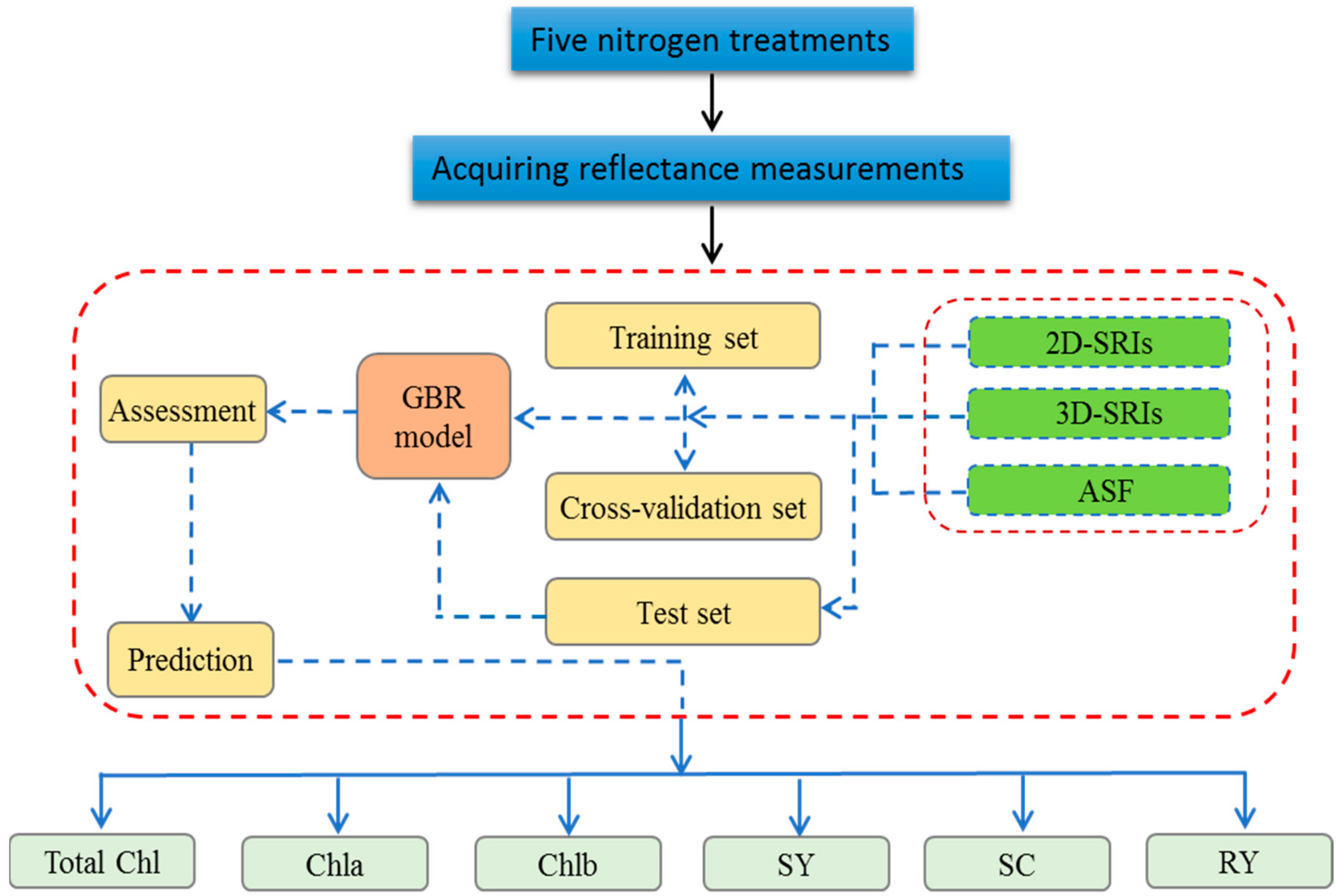
2.4. Gradient Boosting Regression (GBR)

GBR is composed of a group of decision trees used for regression or classification. It is achieved by creating a series of trees, each of which focuses on the prediction residuals of the preceding tree [76]. GBR offers various hyperparameter tuning options and can optimize a variety of loss functions, making it highly adaptable for function fitting. It can be used for both categorical and numerical data, serving as an independent pre-processing step for variables. The ability of GBR to handle missing data is an added advantage. To avoid overfitting, basic trees are constructed in each cycle, which allows for more accurate extrapolation to independent data. The boosting methods generally consist of three components: an additive model, weak learners, and a loss function. This method can capture non-linear relationships, such as wind power curves. It utilizes a range of differentiable loss functions and can learn the connection between input properties iteratively [77]. Gradient boosting machines work by using gradients to identify the limitations of weak models. This is achieved using an iterative strategy with the ultimate goal of combining base learners to minimize forecast errors. Decision trees are combined using an additive model while the loss function is minimized using gradient descent. The GBT ($F_n\left(x_t\right)$) can be defined as the sum of n regression trees, as shown below:

$$F_n\left(x_t\right)={{\displaystyle \sum }}_{i=1}^n{f}_i\left(x_t\right)$$

(5)

where every $f_i\left(x_t\right)$ is a decision tree (regression tree). The ensemble of trees is constructed sequentially by estimating the new decision tree $f_{n+1}\left(x_t\right)$ using the following equation:

$$argmin{{\displaystyle \sum }}_{t}L(y_t.F_n\left(x_t\right)+f_{n+1}\left(x_t\right))$$

(6)

where L(.) is a differentiable loss function. This optimization problem is solved using the steepest descent method.

During training, two criteria were considered: the number of boosting stages to perform (Ns) and the variety of characteristics to take into consideration while choosing the ideal split (Mf). For Ns and Mf, the parameter values were (5, 10, 15, 20, 25) and (‘auto’, ‘sqrt’, ‘log2’), respectively. The top-level model was constructed using the best values obtained after conducting hyperparameter tuning during training. To understand the data processing, Figure 2 depicts a broad flowchart of the methods proposed for indirectly measuring the four studied parameters of sugar beet.

2.5. Data Analysis Software and Datasets

A total of approximately 50 sugar beet samples were used for training and validation. Out of these samples, 80% were used to train and validate the regression model, while the remaining 20% were used to compare the predicted values with the computed values. This was carried out to assess the performance of the model. The model was trained and verified using a technique known as leave-one-out cross-validation (LOOCV). In each trial, LOOCV utilizes the remaining data for training, while excluding one sample for validation. This approach has the potential to reduce the amount of over-fitting that occurs and provide a more precise estimate of the model’s predictive capacity [78]. The program used for data analysis, model creation, and data preparation was Python 3.7.3. To perform tasks involving regression, we investigated the GBR module included in Scikit-learn package version 0.20.2. The data examination was conducted using a machine equipped with an Intel Core i7-3630QM central processing unit operating at 2.4 GHz and with 8 GB of RAM.

2.6. Model Evaluation

The effectiveness of the regression model was evaluated using the following statistical measures: the coefficient of determination (R²) and the root mean square error (RMSE), as shown in Equations (7) and (8) [79,80]. All the parameters being described are as follows: “$V_{act}$” refers to the actual value determined in the laboratory; “$V_p$” stands for the predicted or simulated value; “$V_{ave}$” stands for the average value; and “N” represents all the data points.

$$RMSE=\sqrt{\frac{1}{N}{{\displaystyle \sum }}_{i=1}^N{\left(V_{act}-V_p\right)}^2}$$

(7)

$$R^2=\frac{\sum {\left(V_{act}-V_p\right)}^2}{\sum {\left(V_{act}-V_{ave}\right)}^2}$$

(8)

2.7. Statistical Analysis

A post hoc test (Tukey’s test) at a 0.05 level of probability was used to examine significant differences between the mean values of the measured traits and SRIs under different nitrogen levels. Mean values with the same letter did not differ significantly at p ≤ 0.05. We used simple regression to estimate the relationships between the SRIs and sugar beet parameters. The significance level of R² for these relationships was assessed at p ≤ 0.001, 0.01, and 0.05. The performance of the GBR based on the 2D-SRIs, 3D-SRIs, and ASRIs was evaluated by comparing the values of R² and RMSE. A lower RMSE and higher R² indicate better accuracy of the different models.

3. Results and Discussion

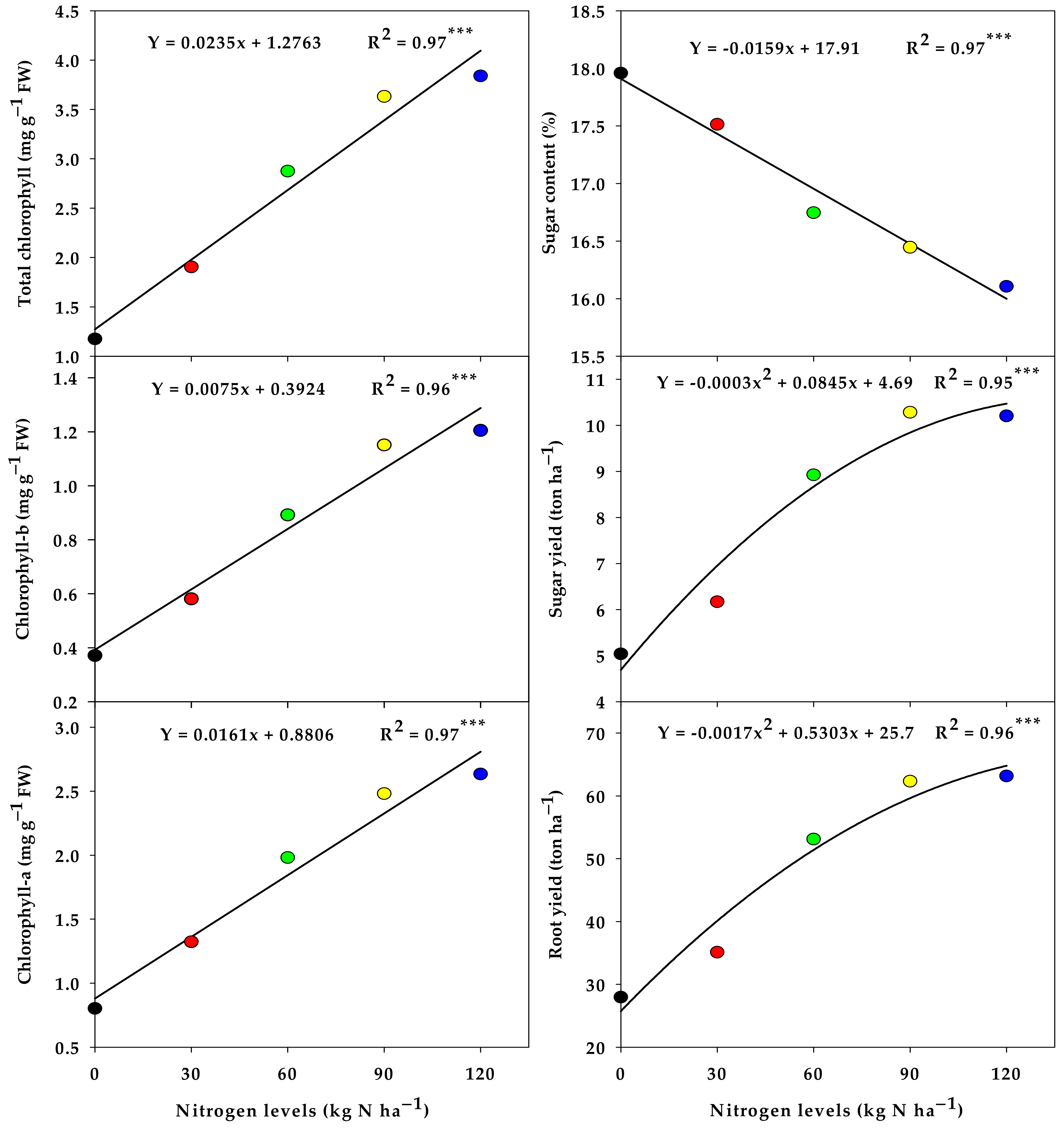
3.1. Response of Chlorophyll Content, Production, and Quality of Sugar Beet to Nitorgen Levels

Table 3. The sum of squares (%) of the combined analysis of variance for chlorophyll a (Cha), chlorophyll b (Chlb), total chlorophyll (Chlt), sugar content (SC), sugar yield (SY), and root yield (RY) influenced by year, nitrogen level (N), and their interaction.

Source of Variation	df	Chla	Chlb	Chlt	SC	SY	RY
		Sum of Squares (%)
Blocks	4	0.15 ns	0.17 ns	0.14 ns	0.32 ns	0.64 ns	0.51 ns
Year (Y)	1	1.90 *	2.70 ***	2.15 **	59.88 ***	14.70 ***	3.92 **
Error-1	4	0.42	0.14	0.31	0.13	0.43	0.30
N	4	92.39 ***	92.20 ***	92.90 ***	37.24 ***	80.44 ***	92.67 ***
N × Y	4	1.80 **	2.45 ***	1.78 **	0.02 ns	0.72 ns	0.17 ns
Error-2	32	3.34	2.46	2.70	2.40	3.08	2.43
Total	49	99.85	99.95	99.85	99.68	99.37	99.49

The share of the sum of squares (%) of the main factors and their interactions is expressed in relation to the sum of squares of the total (100%); ***, **, *, and ^ns indicate significant at p ≤ 0.001, 0.01, 0.05, or not significant, respectively.

displays the influence of years, nitrogen levels (N), and their interactions on the chlorophyll contents (Chla, Chlb, and Chlt) measured at the BBCH 35 growth stage, as well as production (RY and SY) and the quality parameters measured at maturity. The ANOVA revealed that all parameters were significantly affected by the year and nitrogen levels. However, the interaction between them was only significant for the chlorophyll content parameters, not for the production and quality parameters (Table 3).

Regarding the variation in each parameter due to the impacts of the studied factors, ANOVA showed that the N levels had the highest share of variation (80.4%–92.9%), except for SC. In the case of SC, it had a greater variation according to year (59.9%) compared to N levels (37.2%) (Table 3). The year and its interaction with the N level had nearly equal and minimal contributions to the overall variation of Chla (1.90% and 1.80%), Chlb (2.70% and 2.45%), and Chlt (2.15% and 1.78%), respectively. However, the year had a greater share in the variability of RY (3.92%), SY (39.88%), and SC (14.7%) compared to the interaction between year and N level, which accounted for only 0.17%, 0.72%, and 0.02%, respectively (Table 3). These results documented the high importance of nitrogen in sugar beet production since its yield and quality are directly related to N levels. Generally, applying high levels of N leads to enhanced growth and root yield of sugar beet, but it reduces the technical quality of the roots. Under high N levels, the maturity of the sugar beet root slows down, which increases sugar loss and impure sugar content. This is primarily caused by the presence of high levels of harmful nitrogen compounds and melas-forming elements in the roots, such as α-amino-N, sodium, and potassium. These compounds greatly reduce the quality of the sugar beet roots [5,8,9,81]. Conversely, when less nitrogen is applied, the opposite is true, which can be attributed to low levels of nitrogen; the size of the roots significantly shrinks and their moisture content decreases. As a result, there is an increase in SC and significant decreases in RY.

The previous results are confirmed in Figure 1, where there was a significant increase in the chlorophyll contents, yield of roots and sugar as the N levels increased, while the SC decreased. Compared to the control treatment (0 kg N ha⁻¹), nitrogen levels of 30, 60, 90, and 120 kg N ha⁻¹ significantly increased the Chla content by 39.3%, 59.5%, 67.6%, and 69.5%, respectively. They also increased the Chlb content by 36.1%, 58.4%, 67.8%, and 69.2% and the Chlt content by 38.3%, 59.2%, 67.7%, and 69.4%, respectively. Additionally, RY increased by 20.4%, 47.4%, 55.2%, and 55.8%, and SY increased by 18.4%, 43.6%, 51.0%, and 50.6%, respectively. However, SC decreased by 2.5%, 7.2%, 9.2%, and 11.5%, respectively (Figure 3). Because nitrogen plays an important role in the formation of chlorophyll in plants, it could explain why the contents of different types of chlorophyll (chlorophyll a, chlorophyll b, and total chlorophyll) significantly increased with nitrogen levels. Therefore, the chlorophyll content is closely connected to the nitrogen content of the leaves [81,82,83]. Chlorophyll pigments are the most critical substance for absorbing light energy, Chla functions as a pigment that aids in the photochemical process, while Chlb assists in light absorption and the transfer of radiant energy. This vital role of Chl supports the photosynthesis process, which has a significant impact on the growth rate, development, and sugar beet production [84,85]. Thus, the enhancement of the Chl content in plants, induced by sufficient N, could be one of the most important factors contributing to higher yields of roots and sugar under greater levels of N supply, as illustrated in Figure 1. However, nearly all previous studies have reported that excessive N fertilization leads to a significant decrease in sucrose content. This is because it promotes excessive growth of the leaves and crowns, thereby impeding root maturity and increasing nitrate impurities [7,8,9,86]. In this study, the SC decreased by 7.2%, 9.2%, and 11.5% at 60, 90, and 120 kg N ha⁻¹, respectively, compared to 0 kg N ha⁻¹ (Figure 3). The increase in the SC with the treatment of receiving 30 kg N ha⁻¹ or 0 N fertilizers may be attributed to the fact that a lack of nitrogen supply leads to a decrease in root size and moisture content, and thus the SC in the root increases.

Therefore, our results confirm that an elevated amount of nitrogen fertilizer leads to a significant increase in the RY and SY of sugar beet. However, it also has negative effects on root quality by raising harmful nitrogen levels in the root and lowering the SC at harvest. Similar findings have been reported in earlier studies [6,7,8,87]. These studies have found that an optimal rate of N fertilizer is crucial for achieving the maximum RY and optimum SC. However, excessive amounts of nitrogen fertilizer can lead to an increase in RY but a decrease in the SC in the roots. On the contrary, when nitrogen fertilizer amounts are too limited, the opposite is true. Therefore, it is important to apply N fertilizer to sugar beets at a rate that strikes a balance between maximizing the RY and promoting a high SC. However, achieving this target strongly depends on several factors, such as soil type and climate conditions. It is therefore necessary to determine the ideal quantity based mainly on climate and soil conditions. Our results demonstrated that linear functions were effective in fitting the relationship between N levels and chlorophyll content parameters, as well as SC. On the other hand, quadratic functions were found to be effective in fitting the relationship between N levels and the yields of root and sugar (Figure 4). Based on the quadratic functions, 155.9 kg N ha⁻¹ and 140.8 kg N ha⁻¹ are the optimal amounts required for maximizing the RY and SY, respectively, as depicted in Figure 4. This indicates that if the N application rate increases to 156 kg N ha⁻¹, the RY and SC will decrease.

3.2. Response of Published and Newly Spectral Reflectance Indices of Sugar Beet to Different Nitrogen Levels

Table 4. Minimum (Min), maximum (Max), mean, and standard deviation (SD) of different spectral reflectance indices under each nitrogen (N) level. The spectral reflectance for each replicate within each N rate was assessed three times.

Treatment	Statis.	NDI570, 540	NDI686, 620	NAI	NDI780, 550	GI	PRMI	NDI448, 738, 682	NDI448, 684, 738	NDI530, 532, 528
N0	Min	0.0371	−0.0204	0.1283	0.4380	1.0174	1.4088	−0.7806	−0.7484	−0.3330
	Max	0.0599	0.0047	0.2044	0.5334	1.2390	2.2516	−0.7354	−0.4612	−0.3329
	SD	0.0075	0.0088	0.0290	0.0348	0.0762	0.2985	0.0142	0.0799	0.0001
	Mean	0.0482 a	−0.0081 a	0.1664 c	0.4865 d	1.1234 d	1.8215 e	−0.7637 a	−0.5513 a	−0.3329 d
N30	Min	0.0384	−0.0185	0.1458	0.4665	1.0794	1.6443	−0.7883	−0.5809	−0.3330
	Max	0.0545	−0.0062	0.2117	0.5381	1.2105	2.2577	−0.7582	−0.4961	−0.3328
	SD	0.0053	0.0039	0.0214	0.0228	0.0434	0.2008	0.0096	0.0275	0.0001
	Mean	0.0445 a	−0.0126 a	0.1839 c	0.5122 c	1.1657 d	2.0380 d	−0.7762 b	−0.5522 a	−0.3329 d
N60	Min	0.0209	−0.0420	0.1731	0.4951	1.1298	1.8766	−0.8118	−0.6726	−0.3329
	Max	0.0478	−0.0094	0.2553	0.6015	1.4419	3.0213	−0.7674	−0.5311	−0.3327 c
	SD	0.0087	0.0125	0.0247	0.0320	0.1082	0.3525	0.0128	0.0455	0.0001
	Mean	0.0334 b	−0.0248 b	0.2188 b	0.5555 b	1.2918 c	2.4884 c	−0.7934 c	−0.6109 b	−0.3328
N90	Min	0.0117	−0.0578	0.2040	0.5443	1.2142	2.3261	−0.8241	−0.7148	−0.3329
	Max	0.0405	−0.0143	0.2775	0.6236	1.6175	3.3633	−0.7915	−0.5862	−0.3326
	SD	0.0090	0.0147	0.0256	0.0283	0.1284	0.3500	0.0104	0.0421	0.0001
	Mean	0.0267 b	−0.0352 c	0.2315 b	0.5763 b	1.3910 b	2.7466 b	−0.8042 d	−0.6452 b	−0.3328 b
N120	Min	−0.0009	−0.0739	0.2512	0.6102	1.5129	3.1723	−0.8441	−0.7645	−0.3327
	Max	0.0176	−0.0453	0.3020	0.6652	1.8305	4.0204	−0.8181	−0.6912	−0.3325
	SD	0.0066	0.0097	0.0185	0.0188	0.1058	0.2855	0.0083	0.0248	0.0000
	Mean	0.0102 c	−0.0577 d	0.2763 a	0.6319 a	1.6342 a	3.4850 a	−0.8279 e	−0.7206 c	−0.3326 a
Treatment	Statis.	NDI530, 534, 526	NDI536, 538, 534	NDI734, 738, 730	NDI738, 750, 542	NDI590, 588, 594	NDI448, 734, 398	NDI734, 730, 738	NDI536, 538, 532	NDI734, 728, 740
N0	Min	−0.3322	−0.3331	−0.3321	−0.1927	−0.3336	−0.7367	−0.3321	−0.3332	−0.3309
	Max	−0.3315	−0.3330	−0.3315	−0.1760	−0.3332	−0.6725	−0.3315	−0.3331	−0.3292
	SD	0.0002	0.0001	0.0002	0.0056	0.0001	0.0213	0.0002	0.0001	0.0005
	Mean	−0.3318 d	−0.3331 d	−0.3318 e	−0.1831 e	−0.3334 d	−0.7099 a	−0.3318 e	−0.3331 d	−0.3299 d
N30	Min	−0.3319	−0.3331	−0.3319	−0.1848	−0.3335	−0.7438	−0.3319	−0.3331	−0.3301
	Max	−0.3314	−0.3330	−0.3314	−0.1744	−0.3332	−0.7008	−0.3314	−0.3330	−0.3291
	SD	0.0002	0.0000	0.0002	0.0033	0.0001	0.0136	0.0002	0.0000	0.0003
	Mean	−0.3316 d	−0.3330 c	−0.3316 d	−0.1782 d	−0.3333 d	−0.7275 b	−0.3316 d	−0.3330 c	−0.3295 c
N60	Min	−0.3317	−0.3330	−0.3316	−0.1817	−0.3334	−0.7790	−0.3316	−0.3330	−0.3296
	Max	−0.3310	−0.3328	−0.3312	−0.1662	−0.3328	−0.7155	−0.3312	−0.3328	−0.3285
	SD	0.0002	0.0001	0.0001	0.0049	0.0002	0.0188	0.0001	0.0001	0.0003
	Mean	−0.3313 c	−0.3329 b	−0.3314 c	−0.1722 c	−0.3331 c	−0.7530 c	−0.3314 c	−0.3329 b	−0.3289 b
N90	Min	−0.3316	−0.3330	−0.3314	−0.1726	−0.3332	−0.7968	−0.3314	−0.3330	−0.3291
	Max	−0.3306	−0.3328	−0.3310	−0.1619	−0.3327	−0.7485	−0.3310	−0.3327	−0.3281
	SD	0.0003	0.0001	0.0001	0.0034	0.0002	0.0154	0.0001	0.0001	0.0003
	Mean	−0.3310 b	−0.3329 b	−0.3312 b	−0.1681 b	−0.3330 b	−0.7685 d	−0.3312 b	−0.3329 b	−0.3287 b
N120	Min	−0.3308	−0.3329	−0.3311	−0.1639	−0.3328	−0.8220	−0.3311	−0.3329	−0.3283
	Max	−0.3302	−0.3327	−0.3307	−0.1576	−0.3325	−0.7883	−0.3307	−0.3327	−0.3278
	SD	0.0002	0.0000	0.0001	0.0023	0.0001	0.0108	0.0001	0.0000	0.0002
	Mean	−0.3305 a	−0.3328 a	−0.3310 a	−0.1615 a	−0.3327 a	−0.8011 e	−0.3310 a	−0.3328 a	−0.3281 a

The mean value for each parameter with the same letter is not significantly different at different nitrogen levels, according to Tukey’s test at p = 0.05.

displays the minimum, maximum, standard deviation, and means of different SRIs under each N level. It has been observed that the mean values of published and recently developed 3D-SRIs vary significantly between different N levels. This variation reflects the existence of different responses in the spectral reflectance of the sugar beet canopy to varying N levels. For instance, quantitative analyses showed that the mean values of the published SRIs such as NDI_{686, 620}, GI, and PRMI substantially changed from −0.008 to −0.058, 1.123 to 1.634, and 1.822 to 3.485, respectively (Table 3). Additionally, the mean values of newly developed 3D-SRIs such as NDI_{448, 738, 682}, NDI_{448, 684, 738}, and NDI_{530, 532, 528} remarkably changed from −0.828 to 0.764, −0.551 to −0.721, and −0.3329 to −0.3326, respectively. Interestingly, changes in the SRI values were associated with corresponding changes in the measured parameters. These changes would gradually increase or decrease depending on the N levels. Our findings indicate that the different N levels had a significant impact on the spectral reflectance of the plant canopy in the visible (VIS), red-edge, and near-infrared (NIR) regions. Therefore, constructing SRIs using effective wavelengths selected from these three spectral regions could provide a robust tool for estimating sugar beet parameters under various N levels in a rapid and non-destructive manner.

Broadly, the levels of N significantly alter various biophysical and biochemical traits of vegetation canopies. Fortunately, these modifications lead to significant shifts in the canopy’s spectral signatures across the entire spectrum at specific wavelengths [48,56,57,58]. It has been discovered that nitrogen fertilizers have a direct and indirect impact on the spectral reflectance of the plant canopy. Changes in leaf and plant properties such as internal leaf structure, leaf pigments, and biomass are connected to the direct and indirect impacts of N levels. These changes have a significant effect on the spectral signature in the visible and near-infrared ranges [56,57,88,89]. Taking into consideration the aforementioned facts, this research work assessed how different SRIs, which combine various bands from the VIS, red-edge, and NIR regions of the spectrum, responded to varying N levels. According to these findings, all published and newly developed 3D-SRIs demonstrated statistically significant differences among the five N levels.

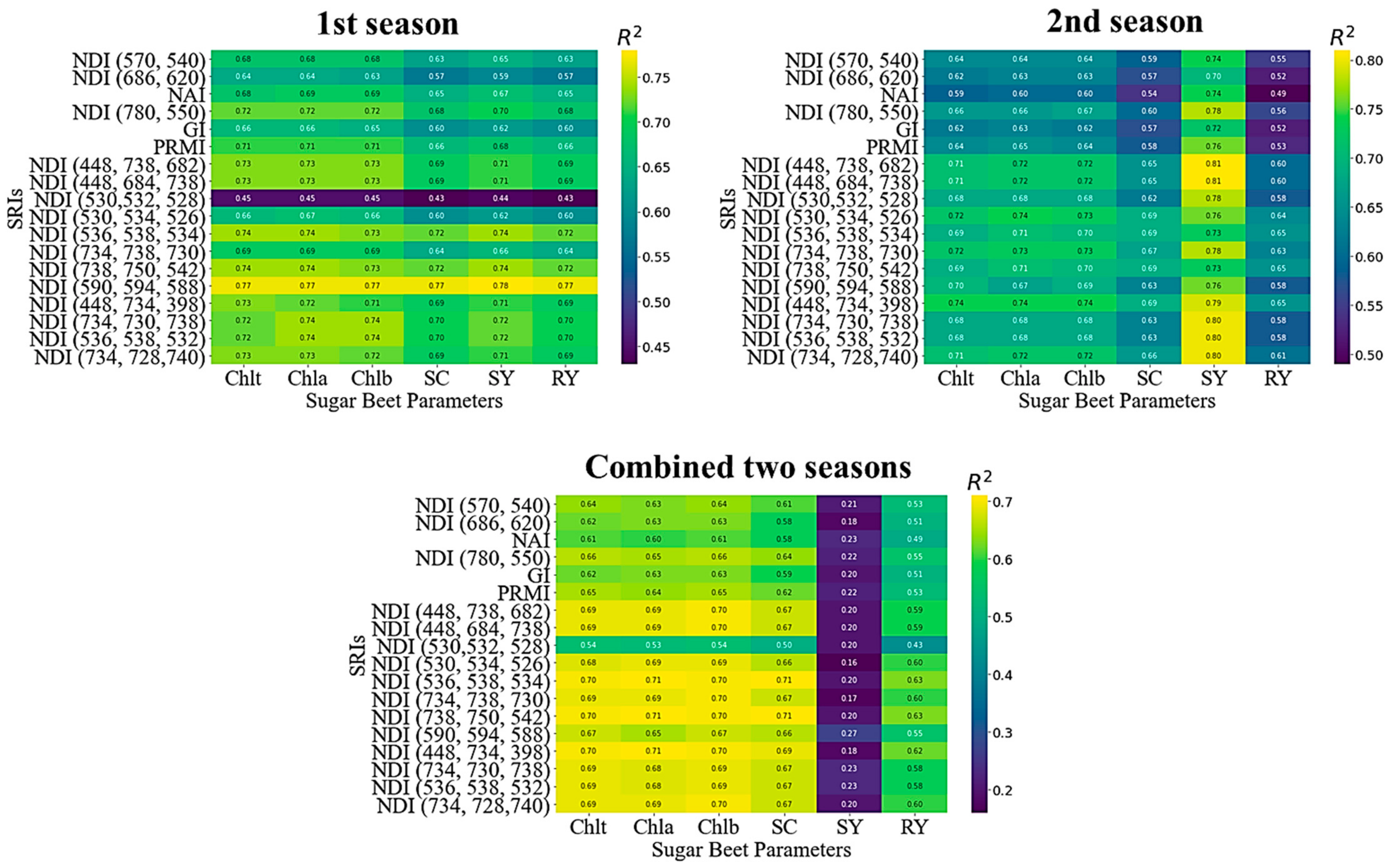
3.3. Potential of the Published and Newly Developed 3D-SRIs to Estimate the Sugar Beet Parameters

The relationships between the measured parameters and various SRIs in the first, second, and combined two seasons are illustrated in Figure 5. The results showed that most of the published and newly developed 3D-SRIs had varying degrees of correlation with different parameters, with R² values ranging from 0.16 to 0.80 (Figure 5). Additionally, the newly developed 3D-SRIs outperformed the previously published ones in estimating the six parameters. The R² values between these indices and all parameters ranged from 0.54 to 0.77 for different Chl contents and from 0.43 to 0.80 for the production and quality parameters (Figure 5). Furthermore, the 3D-SRIs generated from VIS, red-edge, and NIR wavelengths outperformed the other SRIs in detecting changes in Chl content, production, and quality of sugar beet grown under various N levels. For example, NDI_{536, 538, 534}, NDI_{738, 750, 542}, and NDI_{448, 734, 398} provided strong relationships with different Chl content (R² > 0.70), RY (R² > 0.62), and SC (R² > 0.69) when the data of both seasons were combined (Table 4). Many previous studies have utilized all possible combinations of the two bands (contour maps) to identify the optimal SRIs for estimating Chl and N content, N uptake, canopy water content, biomass, and the production of different cultivars grown under various environmental conditions [14,86,88,89,90]. Such studies have reported that contour maps improve the selection of SRIs, making them more reliable to detect the measured parameters. In contrast, other studies have reported that no improvement in the selection of spectral indices was found based on contour map analyses [90]. Few studies have utilized all possible combinations of the three bands (contour maps) to select the most accurate SRIs for estimating N concentration and uptake in wheat and maize crops.

All possible combinations of the three bands were employed to identify the optimized SRIs in our research. Very few studies have utilized 3D contour maps constructed using three-band SRIs to assess these parameters at varying nitrogen levels. Quantifying crop qualities accurately using SRIs that rely on specific wavelengths from a certain spectrum region is challenging due to their sensitivity in evaluating complex development variables like genotypes, growth phase, canopy features, and the environment. Generally, SRIs that incorporate wavelengths from all three spectrum regions are less saturated and, therefore, more resistant to a variety of plant attributes. These attributes include the internal structure of the leaf, increased biomass, nitrogen content, and metabolic factors. This may help explain why the 3D-SRIs outperformed the 2D-SRIs in estimating the parameters examined here.

3.4. Performance of Gradient Boosting Regression Model for Predicting Sugar Beet Parameters

The GBR model was utilized to filter the high-level variables using the 2D-SRIs, 3D-SRIs, and combined types of SRIs and ASRIs (

Table 5. Results of gradient boosting model based on different features extracted from hyperspectral data to predict total chlorophyll (Chlt), chlorophyll a (Chla), chlorophyll b (Chlb), sugar content (SC), sugar yield (SY), and root yield (RY) of sugar beet across various nitrogen levels.

Variable	VIs	Optimal Features	Hyperparameters	Training		Cross-Validation		Testing
				R2	RMSE	R2	RMSE	R2	RMSE
Chlt (mg g−1 FW)	2D	NDI570, 540, NDI686, 620, GI, PRMI, NDI780, 550	(Ns = 300, Mf = log2)	0.990	0.072	0.655	0.345	0.648	0.356
	3D	NDI590, 594, 588, NDI536, 538, 534	(Ns = 100, Mf = sqrt)	0.988	0.080	0.618	0.344	0.732	0.311
	ASRIs	NDI686, 620, NDI590, 588, 594, NDI734, 730, 738, NDI530, 534, 526, NDI536, 534, 538, NDI590, 594, 588	(Ns = 100, Mf = sqrt)	0.989	0.073	0.748	0.304	0.652	0.354
Chla (mg g−1 FW)	2D	PRMI, NDI780, 550, GI	(Ns = 300, Mf = sqrt)	0.989	0.035	0.677	0.152	0.651	0.162
	3D	NDI734, 738, 730, NDI590, 588, 594, NDI536, 538, 534, NDI590, 594, 588, NDI536, 534, 538, NDI536, 538, 534	(Ns = 100, Mf = sqrt)	0.988	0.037	0.655	0.156	0.641	0.148
	ASRIs	NDI536, 538, 534, NDI590, 588, 594, NDI734, 738, 730	(Ns = 200, Mf = log2)	0.989	0.036	0.667	0.159	0.611	0.123
Chlb (mg g−1 FW)	2D	NAI, GI, NDI780, 550, NDI686, 620, NDI570, 540, PRMI	(Ns = 500, Mf = sqrt)	0.989	0.108	0.669	0.493	0.634	0.517
	3D	NDI590, 588, 594, NDI590, 594, 588	(Ns = 100, Mf = auto)	0.985	0.132	0.636	0.479	0.596	0.544
	ASRIs	NDI686, 620, NDI530, 532, 528, NDI734, 738, 730, NDI536, 534, 538, NDI590, 588, 594, NDI448, 738, 682, NDI734, 730, 738, NDI530, 534, 526, NDI590, 594, 588, NDI536, 538, 534	(Ns = 200, Mf = log2)	0.989	0.108	0.691	0.492	0.557	0.569
SC (%)	2D	NDI570, 540, PRMI, NDI780, 550	(Ns = 100, Mf = auto)	0.987	1.721	0.682	6.458	0.667	2.427
	3D	NDI734, 730, 738, NDI734, 738, 730, NDI590, 594, 588, NDI536, 534, 538, NDI536, 538, 534, NDI536, 538, 534	(Ns = 200, Mf = sqrt)	0.989	1.524	0.661	6.637	0.651	7.916
	ASRIs	GI, NDI686, 620, NDI734, 738, 730, NDI590, 588, 594, NDI734, 730, 738, NDI536, 538, 534, NDI536, 534, 538, NDI536, 538, 534	(Ns = 100, Mf = sqrt)	0.989	1.568	0.692	6.120	0.779	6.294
SY (ton ha−1)	2D	NDI686, 620, NDI780, 550, PRMI, NAI	(Ns = 200, Mf = sqrt)	0.998	0.054	0.601	0.523	0.611	0.511
	3D	NDI448, 738, 682, NDI530, 532, 528, NDI448, 682, 738, NDI536, 538, 534, NDI448, 684, 738, NDI530, 534, 526, NDI738, 750, 542	(Ns = 400, Mf = log2)	0.998	0.053	0.503	0.657	0.501	0.649
	ASF	NDI530, 532, 528, NDI 536, 538, 534, NDI686, 620, GI, NDI 734, 738, 730, NDI536, 538, 534, NDI448, 682, 738, NDI734, 728, 740, NDI 448, 684, 738, NDI448, 734, 398, NDI738, 750, 542	(Ns = 100, Mf = sqrt)	0.997	0.062	0.533	0.618	0.518	0.634
RY (ton ha−1)	2D	NDI570, 540, NDI686, 620, NAI, PRMI, NDI780, 550	(Ns = 100, Mf = log2)	0.988	0.264	0.824	0.931	0.815	0.958
	3D	NDI448, 684, 738, NDI734, 730, 738, NDI734, 738, 730, NDI590, 588, 594, NDI590, 594, 588, NDI530, 534, 526, NDI530, 532, 528, NDI536, 538, 534, NDI536, 534, 538, NDI536, 538, 534	(Ns = 500, Mf = log2)	0.990	0.236	0.501	1.341	0.743	1.128
	ASRIs	NAI, NDI780, 550, NDI686, 620, GI, NDI590, 588, 594, NDI734, 738, 730, NDI590, 594, 588, NDI530, 532, 528, NDI734, 730, 738, NDI536, 538, 534, NDI536, 538, 534, NDI530, 534, 526, NDI536, 534, 538	(Ns = 100, Mf = log2)	0.989	0.247	0.522	1.345	0.725	1.167

Where the number of features to take into account when determining the optimal split is Mf, while Ns is the quantity of boosting stages to complete.

). Table 5 illustrates the utilization of 2D-SRIs, 3D-SRIs, and ASRIs in training the GBR model for predicting the various parameters being investigated. The reserved values of the GBR model (independent data) were then compared to the projected values. The analysis and comparison of multivariate techniques indicated significant importance in the predictability of tested crop features. Independent validation is the most reliable method for verifying the accuracy of a regression model because the validation dataset is not utilized during the model-building process. The results demonstrated that GBR-6ASRIs was the most precise prediction model, showing a higher correlation between the Chlt and the outstanding traits. In order to accurately predict the Chlt, this model requires a minimum of two spectral properties. For the training and testing datasets, the outputs of R² were 0.99 (RMSE = 0.073) and 0.65 (RMSE = 0.354), respectively. The GBR-3D-2ASRIs model performed the best when measuring the Chlb, with an R² score of 0.99 (RMSE = 0.132) in the training dataset and 0.60 (RMSE = 0.544) in the testing dataset. Compared to other models, the GBR-7ASRIs model performed better in predicting SC with R² values of 0.99 (RMSE = 1.568) and 0.78 (RMSE = 6.294) for the training and testing datasets, respectively. The RMSE values of the most accurate model (GBR-2D-5ASRIs) for determining the RY under various N levels were 0.26 and 0.96 for the training and testing datasets, respectively. The corresponding R² values were 0.99 and 0.82. According to Elsherbiny et al. [91], several methods were necessary to update regression approaches for accurate prediction. These methods included filtering high-level characteristics and adjusting model hyperparameters. The authors claim that the performance of these updated approaches exceeded expectations. Deep learning algorithms are superior in four key ways: selecting the optimal feature for a color space image, combining image data with information about plants’ environments, data augmentation, and merging different trained deep networks [91]. Zhang et al. [37] discovered that the performance of partial least squares (PLS) regression models based on the novel modified chlorophyll indices MCI (R747, R839), MCI (R861, R884), and MCI (R931, R770) was optimal for accurately predicting Chl levels in sugar beet. The relative root mean square error (RMSE) values for the rapid growth stages of the leaf cluster, sugar growth stage, and sugar accumulation stage were 4.95%, 6.05%, and 5.75%, respectively, in the validation dataset. The corresponding R² values for these stages were 0.83, 0.70, and 0.75, and the corresponding RMSE values were 2.37, 3.11, and 2.78.

4. Conclusions

This study aimed to evaluate the effectiveness of hyperspectral ground-based remote sensing data in predicting the response of various attributes of sugar beet to different levels of nitrogen. The research was conducted at the canopy scale, and it was hypothesized that using machine learning models with novel SRIs could enhance the accuracy of predicting sugar beet parameters. Timely assessment of various plant characteristics is of great importance in efficiently managing agricultural input resources, such as agrochemicals, as well as achieving optimal yield and quality while minimizing environmental impacts. This study investigated the response of various sugar beet parameters to different N levels, as well as examined the ability of various published and newly developed SRIs combined with GBR models to assess these parameters in a timely manner. Generally, the Chl content, RY, and SY gradually increased with increasing N levels; the opposite trend was observed with SC. The newly developed 3D-SRIs, which encompass wavelengths from the VIS, red-edge, and NIR spectrum ranges, were effective enough to accurately estimate various parameters of sugar beet grown under different N levels. Additionally, the GBR had the most precise prediction model, demonstrating a robust correlation with the measured parameters. The GBR-3D-2ASRIs model performed the best when measuring the Chlb with an R² score of 0.99 (RMSE = 0.132) in the training dataset and 0.60 (RMSE = 0.544) in the testing dataset. Compared to the other models, the GBR-7ASRIs model performed better in predicting the SC with R² values of 0.99 (RMSE = 1.568) and 0.78 (RMSE = 6.294) for the training and testing datasets, respectively. In conclusion, the study provides a reliable method for tracking various attributes of sugar beet grown under different N levels. This method can be used with aerial and remote sensing data.

References

1. Jaggard, K.W.; Qi, A.; Milford, G.; Clark, C.; Ober, E.; Walters, C.; Burks, E. Determining the optimal population density of sugar beet crops in England. Int. Sugar J. 2011, 113, 114–119. [Google Scholar]
2. Draycott, A.P.; Christenson, D.R. Nutrients for Sugar Beet Production: Soil–Plant Relationships; CABI Publishing: Wallingford, UK, 2003; 242p. [Google Scholar]
3. Steduto, P.; Hsiao, T.C.; Fereres, E.; Raes, D. Crop Yield Response to Water; FAO: Rome, Italy, 2012. [Google Scholar]
4. Malnou, C.S.; Jaggard, K.W.; Sparkes, D.L. A canopy approach to nitrogen fertilizer recommendation for the sugar beet crop. Eur. J. Agron. 2006, 25, 254–263. [Google Scholar] [CrossRef]
5. Malnou, C.; Jaggard, K.; Sparkes, D. Nitrogen fertilizer and the efficiency of the sugar beet crop in late summer. Eur. J. Agron. 2008, 28, 47–56. [Google Scholar] [CrossRef]
6. Abd El-Lateef, E.M.; Abd El-Salam, M.S.; Elewa, T.A.; Farrag, A.A. Effect of organic manure and nitrogen level on sugar beet (Beta vulgaris Var. Saccharifera L.) yield and root nitrate content. Am. Eurasian J. Agron. 2019, 12, 1–5. [Google Scholar]
7. Leilah, A.A.A.; Khan, N. Interactive Effects of Gibberellic Acid and Nitrogen Fertilization on the Growth, Yield, and Quality of Sugar Beet. Agronomy 2021, 11, 137. [Google Scholar] [CrossRef]
8. Varga, I.; Lončarić, Z.; Kristek, S.; Kulundžić, A.M.; Rebekić, A.; Antunović, M. Sugar Beet Root Yield and Quality with Leaf Seasonal Dynamics in Relation to Planting Densities and Nitrogen Fertilization. Agriculture 2021, 11, 407. [Google Scholar] [CrossRef]
9. Varga, I.; Jović, J.; Rastija, M.; Markulj Kulundžić, A.; Zebec, V.; Lončarić, Z.; Iljkić, D.; Antunović, M. Efficiency and Management of Nitrogen Fertilization in Sugar Beet as Spring Crop: A Review. Nitrogen 2022, 3, 170–185. [Google Scholar] [CrossRef]
10. Franzen, D.W. Delineating nitrogen management zones in a sugarbeet rotation using remote sensing—A review. J. Sugar Beet Res. 2004, 41, 47–60. [Google Scholar] [CrossRef]
11. Varga, I.; Lončarić, Z.; Pospišil, M.; Rastija, M.; Antunović, M. Changes of nitrate nitrogen in sugar beet petioles fresh tissue during season with regard to nitrogen fertilization and plant population. Listy Cukrov. Reparské 2020, 136, 198–204. [Google Scholar]
12. Milford, G.F.J.; Pocock, T.O.; Jaggard, K.W.; Biscoe, P.V.; Armstrong, M.J.; Last, P.J.; Goodman, P.J. An analysis of leaf growth in sugar-beet. 4. The expansion of the leaf canopy in relation to temperature and nitrogen. Ann. Appl. Biol. 1985, 107, 335–347. [Google Scholar] [CrossRef]
13. Jaggard, K.W.; Qi, A. Crop physiology and agronomy. In Sugar Beet; Draycott, A.P., Ed.; Blackwell Publishing: Oxford, UK, 2006; pp. 134–168. [Google Scholar]
14. Elsayed, S.; Barmeier, G.; Schmidhalter, U. Passive reflectance sensing and digital image analysis allows for assessing the biomass and nitrogen status of wheat in early and late tillering stages. Front. Plant Sci. 2018, 9, 1478. [Google Scholar] [CrossRef] [PubMed]
15. Milford, G.F.J.; Travis, K.Z.; Pocock, T.O.; Jaggard, K.W.; Day, W. Growth and dry matter partitioning in sugar-beet. J. Agric. Sci. 1988, 110, 301–308. [Google Scholar] [CrossRef]
16. Salami, M.; Saadat, S. Study of potassium and nitrogen fertilizer levels on the yield of sugar beet in Jolge cultivar. J. Novel Appl. Sci. 2013, 2, 94–100. [Google Scholar]
17. Li, D.; Li, F.; Hu, Y.; Mistele, B.; Schmidhalter, U. Study on the estimation of nitrogen content in wheat and maize canopy based on band optimization of spectral parameters. Spectrosc. Spect. Anal. 2016, 36, 1150–1157. [Google Scholar] [CrossRef]
18. Moran, J.A.; Mitchell, A.K.; Goodmanson, G.; Stockburger, K.A. Differentiation among effects of nitrogen fertilization plant stress responses to gas leaks. Remote Sens. Environ. 2000, 92, 207–217. [Google Scholar]
19. Kaushal, S.S.; Groffman, P.M.; Band, L.E.; Elliott, E.M.; Shields, C.A.; Kendall, C. Tracking nonpoint source nitrogen pollution in human-impacted watersheds. Environ. Sci. Technol. 2011, 45, 8225–8232. [Google Scholar] [CrossRef]
20. Jaggard, K.W.; Qi, A.; Armstrong, M.J. A meta-analysis of sugar beet yield responses to nitrogen fertilizer measured in England since 1980. J. Agric. Sci. 2009, 147, 287–301. [Google Scholar] [CrossRef]
21. Koch, H.; Laufer, D.; Nielsen, O.; Wilting, P. Nitrogen requirement of fodder and sugar beet (Beta vulgaris L.) cultivars under high-yielding conditions of northwestern Europe. Arch. Agron. Soil Sci. 2016, 62, 1222–1235. [Google Scholar] [CrossRef]
22. Tsialtas, J.T.; Maslaris, N. Nitrogen effects on yield, quality and K/Na selectivity of sugar beets grown on clays under semi-arid, irrigated conditions. Int. J. Plant Prod. 2013, 7, 355–372. [Google Scholar]
23. Mekdad, A.A.A.; Rady, M.M. Response of Beta vulgaris L. to nitrogen and micronutrients in dry environment. Plant Soil Environ. 2016, 62, 23–29. [Google Scholar] [CrossRef]
24. Carter, G.A. Reflectance wavebands and indices for remote estimation of photosynthesis and stomatal conductance in pine canopies. Remote Sens. Environ. 1998, 63, 61–72. [Google Scholar] [CrossRef]
25. Clevers, J.G.P.W.; Gitelson, A.A. Remote estimation of crop and grass chlorophyll and nitrogen content using red-edge bands on Sentinel-2 and -3. Int. J. Appl. Earth Obs. Geoinf. 2013, 23, 344–351. [Google Scholar] [CrossRef]
26. Wang, Y.; Wang, D.J.; Shi, P.H.; Omass, K. Estimating rice chlorophyll content and leaf nitrogen concentration with a digital still color camera under natural light. Plant Methods 2014, 10, 36. [Google Scholar] [CrossRef] [PubMed]
27. Meskinivishkaee, F.; Mohammadi, M.H.; Neyshabouri, M.R.; Shekari, F. Evaluation of canola chlorophyll index and leaf nitrogen under wide range of soil moisture. Int. Agrophys. 2015, 29, 83–90. [Google Scholar] [CrossRef]
28. Manderscheid, R.; Pacholski, A.; Weigel, H.J. Effect of free air carbon dioxide enrichment combined with two nitrogen levels on growth, yield and yield quality of sugar beet: Evidence for a sink limitation of beet growth under elevated CO2. Eur. J. Agron. 2010, 32, 228–239. [Google Scholar] [CrossRef]
29. Richardson, A.D.; Duigan, S.; Berlyn, G. An evaluation of noninvasive methods to estimate foliar chlorophyll content. New Phytol. 2002, 153, 185–194. [Google Scholar] [CrossRef]
30. Jin, S.; Wang, P.; Zhao, K.; Yang, Y.; Yao, S.; Jiang, D. Characteristics of gas exchange and chlorophyll fluorescence in different position leaves at booting stage in rice plants. Rice Sci. 2004, 11, 283–289. [Google Scholar]
31. Marenco, R.A.; Antezana-Vera, S.A.; Nascimento, H.C.S. Relationship between specific leaf area, leaf thickness, leaf water content and SPAD—502 readings in six Amazonian tree species. Photosynthetica 2009, 47, 184–190. [Google Scholar] [CrossRef]
32. El-Hendawy, S.; Elsayed, S.; Al-Suhaibani, N.; Alotaibi, M.; Tahir, M.U.; Mubushar, M.; Attia, A.; Hassan, W.M. Use of Hyperspectral Reflectance Sensing for Assessing Growth and Chlorophyll Content of Spring Wheat Grown under Simulated Saline Field Conditions. Plants 2021, 10, 101. [Google Scholar] [CrossRef]
33. Chen, X.W.; Dong, Z.Y.; Liu, J.B.; Wang, H.Y.; Zhang, Y.; Chen, T.Q.; Du, Y.C.; Shao, L.; Xie, J.C. Hyperspectral characteristics and quantitative analysis of leaf chlorophyll by reflectance spectroscopy based on a genetic algorithm in combination with partial least squares regression. Spectrochim. Acta Part A Mol. Biomol. Spectrosc. 2020, 243, 118786. [Google Scholar] [CrossRef]
34. Marang, I.J.; Filippi, P.; Weaver, T.B.; Evans, B.J.; Whelan, B.M.; Bishop, T.F.A.; Murad, O.F.M.; Al-Shammari, D.; Roth, G. Machine Learning Optimised Hyperspectral Remote Sensing Retrieves Cotton Nitrogen Status. Remote Sens. 2021, 13, 1428. [Google Scholar] [CrossRef]
35. Tao, H.; Feng, H.; Xu, L.; Miao, M.; Long, H.; Yue, J.; Li, Z.; Yang, G.; Yang, X.; Fan, L. Estimation of Crop Growth Parameters Using UAV-Based Hyperspectral Remote Sensing Data. Sensors 2020, 20, 1296. [Google Scholar] [CrossRef] [PubMed]
36. Yang, H.; Li, F.; Hu, Y.; Yu, K. Hyperspectral indices optimization algorithms for estimating canopy nitrogen concentration in potato (Solanum tuberosum L.). Int. J. Appl. Earth Obs. Geoinf. 2021, 102, 102416. [Google Scholar] [CrossRef]
37. Zhang, J.; Tian, H.; Wang, D.; Li, H.; Mouazen, A.M. A novel spectral index for estimation of relative chlorophyll content of sugar beet. Comput. Electron. Agric. 2021, 184, 106088. [Google Scholar] [CrossRef]
38. Geipel, J.; Link, J.; Claupein, W. Combined spectral and spatial modeling of corn yield based on aerial images and crop surface models acquired with an unmanned aircraft system. Remote Sens. 2014, 6, 10335–10355. [Google Scholar] [CrossRef]
39. Hamblin, J.; Knight, R.; Atkinson, M.J. The influence of systematic micro-environmental variation on individual plant yield within selection plots. Euphytica 1978, 27, 497–503. [Google Scholar] [CrossRef]
40. Köksal, E.S.; Güngör, Y.; Yildirim, Y.E. Spectral reflectance characteristics of sugar beet under different levels of irrigation water and relationships between growth parameters and spectral indexes. Irrig. Drain. 2011, 60, 187–195. [Google Scholar] [CrossRef]
41. Kira, O.; Linker, R.; Gitelson, A.A. Non-destructive estimation of foliar chlorophyll and carotenoid contents: Focus on informative spectral bands. J. Appl. Earth Observ. Geoinf. 2015, 38, 251–260. [Google Scholar] [CrossRef]
42. Zhao, Y.X.; Yan, C.H.; Lu, S.; Wang, P.; Qiu, G.Y.; Li, R.L. Estimation of chlorophyll content in intertidal mangrove leaves with different thicknesses using hyperspectral data. Ecol. Ind. 2019, 106, 105511. [Google Scholar] [CrossRef]
43. Romero, A.P.; Alarcón, A.; Valbuena, R.I.; Galeano, C.H. Physiological assessment of water stress in potato using spectral information. Front. Plant Sci. 2017, 8, 1608. [Google Scholar] [CrossRef]
44. Miloš, B.; Josef, H.; Jana, M.; Kateřina, S.; Alica, K. Dehydration-induced changes in spectral reflectance indices and chlorophyllfluorescence of Antarctic lichens with different thalluscolor, and intrathallinephotobiont. Acta Physiol. Plant. 2018, 40, 177. [Google Scholar] [CrossRef]
45. Jay, S.; Gorretta, N.; Morel, J.; Maupas, F.; Bendoula, R.; Rabatel, G.; Dutartre, D.; Comar, A.; Baret, F. Estimating leaf chlorophyll content in sugar beet canopies using millimeter- to centimeter-scale reflectance imagery. Remote Sens. Environ. 2017, 198, 173–186. [Google Scholar] [CrossRef]
46. Datt, B. A new reflectance index for remote sensing of chlorophyll content in higher plants: Tests using Eucalyptus leaves. J. Plant Physiol. 1999, 154, 30–36. [Google Scholar] [CrossRef]
47. Amirruddin, A.D.; Muharam, F.M.; Ismail, M.H.; Ismail, M.F.; Tan, N.P.; Karam, D.S. Hyperspectral remote sensing for assessment of chlorophyll sufficiency levels in mature oil palm (Elaeis guineensis) based on frond numbers: Analysis of decision tree and random forest. Comput. Electron. Agric. 2020, 169, 105–221. [Google Scholar] [CrossRef]
48. Gitelson, A.A. Nondestructive estimation of foliar pigment (chlorophylls, carotenoids, and anthocyanins) contents. In Hyperspectral Remote Sensing of Vegetation; Thenkabail, P.S., Lyon, J.G., Huete, A., Eds.; CRC Press: London, UK; New York, NY, USA, 2011; pp. 141–166. [Google Scholar]
49. Lu, S.; Lu, F.; You, W.; Wang, Z.; Liu, Y.; Omasa, K. A robust vegetation index for remotely assessing chlorophyll content of dorsiventral leaves across several species in different seasons. Plant Methods 2018, 14, 15. [Google Scholar] [CrossRef]
50. Dong, T.F.; Liu, J.G.; Shang, J.L.; Qian, B.D.; Ma, B.L.; Kovacs, M.J.; Walters, D.; Jiao, X.F.; Geng, X.Y.; Shi, Y.C. Assessment of red-edge vegetation indices for crop leaf area index estimation. Remote Sens. Environ. 2019, 222, 133–143. [Google Scholar] [CrossRef]
51. Mistele, B.; Schmidhalter, U. Spectral measurements of the total aerial N and biomass dry weight in maize using a quadrilateral-view optic. Field Crops Res. 2008, 106, 94–103. [Google Scholar] [CrossRef]
52. Dray, F.A., Jr.; Center, T.D.; Mattison, E.D. In situ estimates of waterhyacinth leaf tissue nitrogen using a SPAD-502 chlorophyll meter. Aquat. Bot. 2012, 100, 72–75. [Google Scholar] [CrossRef]
53. Adelabu, S.; Mutanga, O.; Adam, E. Evaluating the impact of red-edge band from rapideye image for classifying insect defoliation levels. ISPRS J. Photogramm. Remote Sens. 2014, 95, 34–41. [Google Scholar] [CrossRef]
54. Evangelides, C.; Nobajas, A. Red-edge normalised difference vegetation index (NDVI 705) from sentinel-2 imagery to assess post-fire regeneration. Remote Sens. Appl. Soc. Environ. 2020, 17, 100283. [Google Scholar]
55. Ray, S.S.; Das, G.; Singh, J.P.; Panigrahy, S. Evaluation of hyperspectral indices for LAI estimation anddiscrimination of potato crop under different irrigationtreatments. Int. J. Remote Sens. 2006, 27, 5373–5387. [Google Scholar] [CrossRef]
56. Hasituya; Li, F.; Elsayed, S.; Hu, Y.; Schmidhalter, U. Passive reflectance sensing using optimized two- and three-band spectral indices for quantifying the total nitrogen yield of maize. Comput. Electron. Agric. 2021, 173, 105403. [Google Scholar] [CrossRef]
57. Li, F.; Li, D.; Elsayed, S.; Hu, Y.; Schmidhalter, U. Using optimized three-band spectral indices to assess canopy N uptake incorn and wheat. Eur. J. Agron. 2021, 127, 126286. [Google Scholar] [CrossRef]
58. El-Hendawy, S.; Dewir, Y.H.; Elsayed, S.; Schmidhalter, U.; Al-Gaadi, K.; Tola, E.; Refay, Y.; Tahir, M.U.; Hassan, W.M. CombiningHyperspectral Reflectance Indicesand Multivariate Analysis to Estimate Different Units of Chlorophyll Content of Spring Wheat under Salinity Conditions. Plants 2022, 11, 456. [Google Scholar] [CrossRef] [PubMed]
59. Beltrán, N.H.; Duarte-Mermoud, M.A.; Salah, S.A.; Bustos, M.A.; Peña-Neira, A.I.; Loyola, E.A.; Jalocha, J.W. Feature selection algorithms using Chilean wine chromatograms as examples. J. Food Eng. 2005, 67, 483–490. [Google Scholar] [CrossRef]
60. Guyon, I.; Elisseeff, A. An Introduction to Variable and Feature Selection. J. Mach. Learn. Res. 2003, 3, 1157–1182. [Google Scholar]
61. Schuize, F.H.; Wolf, H.; Jansen, H.; Vander, V.P. Applications of artificial neural networks in integrated water management: Fiction or future? Water Sci. Technol. 2005, 52, 21–31. [Google Scholar] [CrossRef]
62. Strobl, C.; Boulesteix, A.-L.; Kneib, T.; Augustin, T.; Zeileis, A. Conditional variable importance for random forests. BMC Bioinform. 2008, 9, 307. [Google Scholar] [CrossRef]
63. Glorfeld, L.W. A methodology for simplification and interpretation of backpropagation-based neural network models. Expert Syst. Appl. 1996, 10, 37–54. [Google Scholar] [CrossRef]
64. Melis, G.; Dyer, C.; Blunsom, P. On the state of the art of evaluation in neural language models. arXiv 2017, arXiv:1707.05589. [Google Scholar]
65. Bergstra, J.; Yamins, D.; Cox, D. Making a science of model search: Hyperparameter optimization in hundreds of dimensions for vision architectures. In Proceedings of the 30th International Conference on Machine Learning (ICML), Atlanta, GA, USA, 16–21 June 2013; pp. 115–123. [Google Scholar]
66. Wu, J.; Chen, X.-Y.; Zhang, H.; Xiong, L.-D.; Lei, H.; Deng, S.-H. Hyperparameter optimization for machine learning models based on Bayesian optimization. J. Electron. Sci. Technol. 2019, 17, 26–40. [Google Scholar]
67. Doorenbos, I.; Kassam, A. Yield Response to Water; F.A.O Irrigation and Drainage Paper No. 33; FAO: Rome, Italy, 1979. [Google Scholar]
68. Lichtenthaler, H.K.; Wellburn, A.R. Determinations of total carotenoids and chlorophylls a and b of leaf extracts in differentsolvents. Biochem. Soc. Trans. 1983, 603, 591–592. [Google Scholar] [CrossRef]
69. Carruthers, A.; Oldfield, J.F.T. Methods for the assessment of beet quality. Int. Sugar J. 1960, 63, 72–74. [Google Scholar]
70. Elsayed, S.; El-Gozayer, K.; Allam, A.; Schmidhalter, U. Passive reflectance sensing using regression and multivariate analysis to estimate biochemical parameters of different fruits kinds. Sci. Hortic. 2019, 243, 21–33. [Google Scholar] [CrossRef]
71. Elsayed, S.; Galal, H.; Allam, A.P.; Schmidhalter, U. Passive reflectance sensing anddigital image analysis for assessing quality parameters of mango fruits. Sci. Hortic. 2016, 212, 136–147. [Google Scholar] [CrossRef]
72. Rouse, J.W.; Haas, R.H.; Schell, J.A.; Deering, D.W.; Harlan, J.C. Monitoring the Vernal Advancement of Retro Gradation of Natural Vegetation; NASA/GSFC, Type lll, Final Report; NASA/GSFC: Greenbelt, MD, USA, 1974. [Google Scholar]
73. Gutierrez, M.; Reynolds, M.P.; Raun, W.R.; Stone, M.L.; Klatt, A.R. Spectral water indices for assessing yield in elite bread wheat genotypes in well irrigated, water stressed, and high temperature conditions. Crop Sci. 2010, 50, 197–214. [Google Scholar] [CrossRef]
74. Acharya, U.K.; Subedi, P.P.; Walsh, K.B.; McGlasson, W.B. Estimation of fruit maturation and ripening using spectral indices. Acta Hortic. 2016, 1119, 265–272. [Google Scholar] [CrossRef]
75. Nagy, A.; Riczu, P.; Tamás, J. Spectral evaluation of apple fruit ripening and pigment content alteration. Sci. Hortic. 2016, 201, 256–264. [Google Scholar] [CrossRef]
76. Gilbert, C.; Browell, J.; McMillan, D. Leveraging Turbine-Level Data for Improved ProbabilisticWind Power Forecasting. IEEE Trans. Sustain. Energy 2019, 11, 1152–1160. [Google Scholar]
77. Elith, J.; Leathwick, J.R.; Hastie, T. A Working Guide to Boosted Regression Trees. J. Anim. Ecol. 2008, 77, 802–813. [Google Scholar] [CrossRef]
78. Zhu, J.; Huang, Z.H.; Sun, H.; Wang, G.X. Mapping forest ecosystem biomass density for Xiangjiang river basin by combining plot and remote sensing data and comparing spatial extrapolation methods. Remote Sens. 2017, 9, 241. [Google Scholar] [CrossRef]
79. Malone, B.P.; Styc, Q.; Minasny, B.; McBratney, A.B. Digital soil mapping of soil carbon at the farm scale: A spatial downscaling approach in consideration of measured and uncertain data. Geoderma 2017, 290, 91–99. [Google Scholar] [CrossRef]
80. Saggi, M.K.; Jain, S. Reference evapotranspiration estimation and modeling of the Punjab Northern India using deep learning. Comput. Electron. Agric. 2019, 156, 387–398. [Google Scholar] [CrossRef]
81. Kristek, S.; Kristek, A.; Evačić, M. Influence of nitrogen fertilization on sugar beet root yield and quality. Cereal Res. Commun. 2008, 36, 371–374. [Google Scholar]
82. Wang, Z.; Skidmore, A.K.; Darvishzadeh, R.; Wang, T. Mapping forest canopy nitrogen content by inversion of coupled leaf-canopy radiative transfer models from airborne hyperspectral imagery. Agric. For. Meteorol. 2018, 253–254, 247–260. [Google Scholar] [CrossRef]
83. Zarco-Tejada, P.J.; Hornero, A.; Beck, P.S.A.; Kattenborn, T.; Kempeneers, P.; Hernández-Clemente, R. Chlorophyll content estimation in an open-canopy conifer forest with Sentinel-2A and hyperspectral imagery in the context of forest decline. Remote Sens. Environ. 2019, 223, 320–335. [Google Scholar] [CrossRef]
84. Zhang, G.; Liu, Q.; Zhang, Z.; Ci, D.; Zhang, J.; Xu, Y.; Guo, Q.; Xu, M.; He, K. Effect of reducing nitrogen fertilization and adding organic fertilizer on net photosynthetic rate, root nodules and yield in peanut. Plants 2023, 12, 2902. [Google Scholar] [CrossRef]
85. Wang, B.F.; Yu, Z.Y.; Cheng, J.P.; Li, Y.; Zhang, Z.S.; Yang, X.L. Research progress on the effect of nitrogen on rice yield and quality formation. J. Huazhong Agric. Univ. 2022, 41, 76–83. [Google Scholar]
86. Yin, H.; Li, B.; Wang, X.; Xi, Z. Effect of ammonium and nitrate supplies on nitrogen and sucrose metabolism of cabernet sauvignon (Vitis vinifera cv.). J. Sci. Food Agric. 2020, 100, 5239–5250. [Google Scholar] [CrossRef]
87. Li, J.; Liu, X.; Yao, Q.; Xu, L.; Li, W.; Tan, W.; Wang, Q.; Xing, W.; Liu, D. Tolerance and adaptation characteristics of sugar beet (Beta vulgaris L.) to low nitrogen supply. Plant Signal. Behav. 2023, 18, 2159155. [Google Scholar] [CrossRef]
88. Li, F.; Mistele, B.; Hu, Y.; Chen, X.; Schmidhalter, U. Comparing hyperspectral index optimization algorithms to estimate aerial N uptake using multi-temporal winter wheat datasets. Agric. For. Meteorol. 2013, 180, 44–57. [Google Scholar] [CrossRef]
89. Li, F.; Mistele, B.; Hu, Y.; Chen, X.; Schmidhalter, U. Optimising three-band spectral indices to assess aerial N concentration, N uptake and aboveground biomass of winter wheat remotely in China and Germany. ISPRS J. Photogramm. Remote Sens. 2014, 92, 112–123. [Google Scholar] [CrossRef]
90. Barmeier, G.; Schmidhalter, U. High-throughput field phenotyping of leaves, leaf sheaths, culms and ears of spring barley cultivars at anthesis and dough Ripeness. Front. Plant Sci. 2017, 8, 1920. [Google Scholar] [CrossRef] [PubMed]
91. Elsherbiny, O.; Fan, Y.; Zhou, L.; Qiu, Z. Fusion of feature selection methods and regression algorithms for predicting the canopy water content of rice based on hyperspectral data. Agriculture 2021, 11, 51. [Google Scholar] [CrossRef]
Figure 1. Correlation matrices display the estimated (R2) values for all potential three-band spectral combinations with total chlorophyll (Chlt), chlorophyll a (Chla), chlorophyll b (Chlb), sugar content, sugar yield (SY), and root yield (RY) across two successive seasons.
Agronomy 13 02743 g001
Figure 2. Flowchart illustrating a general overview of the methods presented for indirectly quantifying sugar beet parameters, including total chlorophyll, chlorophyll-a (Chla), chlorophyll-b (Chlb), sugar content (SC), sugar yield (SY), and root yield (RY).
Agronomy 13 02743 g002
Figure 3. Response of chlorophyll-a, chlorophyll-b, total chlorophyll, root yield, sugar yield, and sugar content to different nitrogen levels. Bars followed by the same letter do not differ statistically according to Tukey’s test at p = 0.05.
Agronomy 13 02743 g003
Figure 4. Functional relationships between nitrogen levels and different sugar beet parameters. *** indicates significant at p < 0.001.
Agronomy 13 02743 g004
Figure 5. Coefficient of determinations (R2) for the linear regression of various spectral reflectance indices (SRIs) with total chlorophyll (Chlt), chlorophyll a (Chla), chlorophyll b (Chlb), root yield (RY), sugar yield (SY), and sugar content (SC) of sugar beet across five nitrogen levels for each season and combined two years.
Agronomy 13 02743 g005