Abstract
Constructing optical image time series for cropland monitoring requires a cloud removal method that accurately restores cloud regions and eliminates discontinuity around cloud boundaries. This paper describes a two-stage hybrid machine learning-based cloud removal method that combines Gaussian process regression (GPR)-based predictions with image blending for seamless optical image reconstruction. GPR is employed in the first stage to generate initial prediction results by quantifying temporal relationships between multi-temporal images. GPR predictive uncertainty is particularly combined with prediction values to utilize uncertainty-weighted predictions as the input for the next stage. In the second stage, Poisson blending is applied to eliminate discontinuity in GPR-based predictions. The benefits of this method are illustrated through cloud removal experiments using Sentinel-2 images with synthetic cloud masks over two cropland sites. The proposed method was able to maintain the structural features and quality of the underlying reflectance in cloud regions and outperformed two existing hybrid cloud removal methods for all spectral bands. Furthermore, it demonstrated the best performance in predicting several vegetation indices in cloud regions. These experimental results indicate the benefits of the proposed cloud removal method for reconstructing cloud-contaminated optical imagery.
1. Introduction
The growing population and climate change present significant challenges to food security [1]. The increasing climate variability has a significant impact on food production, emphasizing growing needs for sustainable agricultural management to meet food security needs [2]. Consistent cropland monitoring and thematic information extraction are essential for sustainable agricultural management [3]. In this context, remote sensing imagery is regarded as an important source of information owing to its ability to provide periodic thematic information in croplands. The representative thematic information derived from remote sensing imagery includes crop type maps [4,5] and crop yield prediction information [6,7,8]. Remote sensing-based crop monitoring often requires image time series to extract information on the growth cycles of crops of interest. However, the acquisition of optical remote sensing imagery is greatly affected by atmospheric conditions, making it challenging to collect multi-temporal cloud-free optical images. The presence of clouds and cloud shadows in optical imagery greatly reduces the usability of data for multi-temporal cropland monitoring. When optical imagery contains clouds and cloud shadows, cloud-contaminated regions are first detected and then masked out in the imagery. Representative cloud detection tools include Sen2Cor [9], MACCS-ATCOR Joint Algorithm (MAJA) [10], and AgroShadow [11]. Even though cloud regions are accurately detected, these regions are excluded from further analysis. Thus, image reconstruction or gap-filling in cloud regions [12,13] is required in order to increase the number of available optical images for cropland monitoring.
This study defines cloud removal as the reconstruction of missing information in clouds and cloud shadows. From a methodological standpoint, cloud removal can be grouped into spatial, spectral, temporal, and hybrid approaches depending on the types of available auxiliary information [12,13,14,15,16]. The spatial approach predicts missing information using information from cloud-free regions within the same image [17,18,19]. The spectral approach utilizes complementary information from other spectral bands unaffected by clouds for image reconstruction [20,21,22]. The temporal approach utilizes images acquired at different times in the same geographical region as auxiliary information to reconstruct cloud regions. Regression-based methods [23,24,25,26,27] have mainly been applied due to their ability to quantify complex temporal relationships between the reference date (the date on which an auxiliary image is acquired) and the prediction date (the date on which the cloud-contaminated image is acquired). As the three approaches mentioned above utilize correlation information in only one domain, their predictive performance depends heavily on the correlation strength of the considered domain [12]. The hybrid approach combines the advantages of individual methods for cloud removal. As a representative hybrid method, the neighborhood similar pixel interpolator (NSPI) [28] was developed to fill gaps due to the scan-line corrector failure of the Landsat ETM+ sensor [29] and has been further modified for cloud removal.
Even though any hybrid method may be applied to cloud removal, prediction results usually contain spectral discontinuity between cloud-free and reconstructed regions [27]. Thus, a specific procedure to remove seams around cloud boundaries is required to generate continuous spectral patterns in prediction results. To this end, Lin et al. [30] and Hue et al. [31] first replaced cloud masks in a target image with reference image patches. Poisson blending was then applied to remove seams around reconstructed regions. However, prediction errors may increase when the spectral differences between the reference and prediction dates are substantial. A critical factor in image blending-based seam removal is the error propagation problem. Since seam removal is primarily based on initial prediction results, errors in initial predictions affect the quality of seam removal accordingly. Thus, for seam removal, it is essential to generate initial predictions with high accuracy within cloud regions.
Regarding the generation of initial predictions with high accuracy, machine learning-based regression has great potential for cloud removal from optical remote sensing images because auxiliary information from pixels with the same land-cover type and spatial structures is utilized to capture complex relationships. Among a plethora of machine learning-based regression methods, Gaussian process regression (GPR) has achieved superior predictive performance in regression tasks involving remote sensing images [32,33,34]. In addition, it has been successfully applied to cloud removal [27,35,36,37]. Recently, Park et al. [38] also reported that GPR was robust to variations in land-cover types and spectral changes in training samples, achieving better prediction accuracy compared to the random forest and support vector regression models. However, GPR has not yet been applied as an initial prediction generator within the hybrid cloud removal approach.
Furthermore, image blending has been applied directly to a postprocessor for seam elimination in existing cloud removal studies, without further modification of the initial prediction results. To the best of our knowledge, regression-based initial predictions have not been logically interconnected to image blending within an integrated framework. Instead, the two procedures have been separately applied to cloud removal.
This study presents a two-stage hybrid approach to thick cloud removal from optical remote sensing images. The proposed cloud removal method combines a GPR-based temporal method with a Poisson blending-based spatial method. The former is applied to generate initial prediction with higher accuracy, and the latter is employed to eliminate discontinuity around cloud boundaries. The final prediction results containing reflectance values continuously corrected from the cloud boundary to the interior are finally obtained by applying Poisson blending. The main contribution of this approach is to provide a novel pipeline for cloud removal that includes a modification procedure for GPR-based initial predictions that is specific to Poisson blending-based discontinuity elimination. As initial prediction results are directly fed into the Poisson blending procedure, uncertainty in GPR-based prediction affects the gradient computation for discontinuity elimination. In this work, uncertainty-weighted predictions are used as input for the gradient computation to alleviate the impact of the prediction uncertainty on Poisson blending. The uncertainty-weighted scheme in particular is proposed because GPR provides the prediction uncertainty, and the gradient information (not the original image values) is considered within Poisson blending. The potential of the proposed approach was demonstrated via cloud removal experiments using Sentinel-2 images of two agricultural sites.
2. Methods
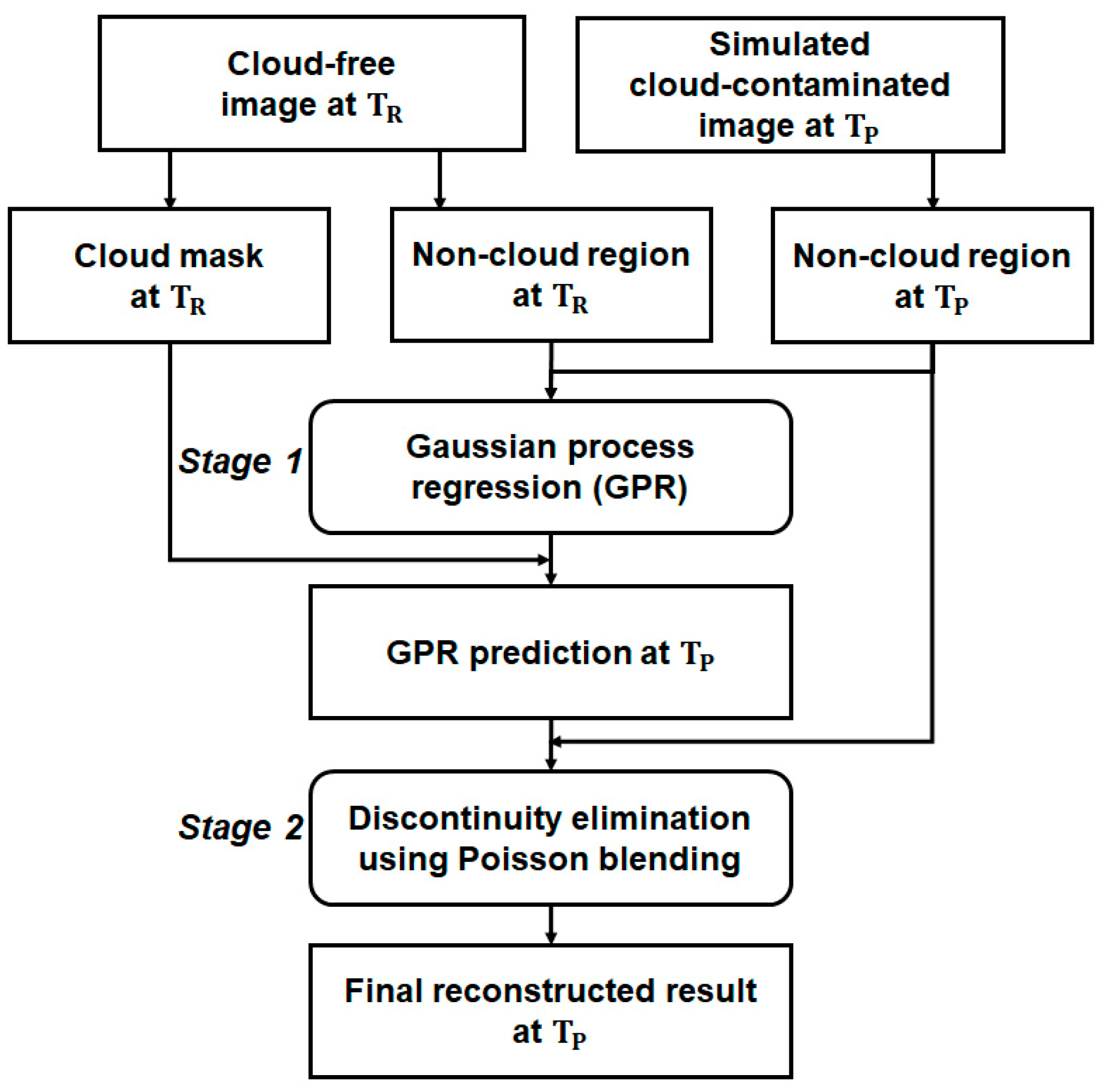
In this study, cloud removal is undertaken to reconstruct cloud-contaminated remote sensing imagery from the prediction date () using the cloud-free imagery from the reference date (). The two-stage hybrid cloud removal method proposed in this study combines GPR-based predictions with Poisson blending-based discontinuity elimination (Figure 1).
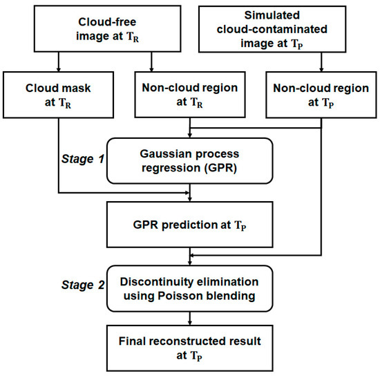
Figure 1.
Schematic diagram of the processing flow of the two-stage cloud removal method proposed in this study (: reference date; : prediction date).
2.1. Initial Prediction Using Gaussian Process Regression
GPR first quantifies the relationships between and using training samples extracted from non-cloud regions both in reference and prediction images. The reflectance values in the cloud masks of the target imagery at for each spectral band are then predicted using the quantified relationships and reflectance values from the cloud masks in the reference imagery. The initial prediction result based on GPR at is an image in which cloud masks are replaced with GPR-based prediction results, while non-cloud regions are retained.
GPR learns a probability distribution over functions via a stochastic Gaussian process (GP) [39,40]. In GPR, given a set of training samples, the output is formulated as the sum of some unknown latent function at an input , and the Gaussian noise with zero mean and variance :
Unlike conventional parametric regression models, the latent function is regarded as a random variable following a particular distribution. In GPR, is assumed to be distributed as a GP, which is defined as a collection of random variables, any finite number of which have a joint Gaussian distribution [39] (p. 13). A GP is completely specified by its mean function and covariance function :
By combining the zero mean GP prior and the Gaussian likelihood computed from training samples, the posterior distribution over the unknown output for the new observation can be analytically computed within a Bayesian framework. After computing and , the predictive mean () and the predictive variance () at the new observation are finally obtained, as follows:
where is an vector.
The attractive advantage of GPR over other regression models is its ability to provide prediction uncertainty estimates (i.e., the predictive variance in Equation (4)) together with prediction values.
The covariance function in Equation (2) is specified by the kernel function measuring the similarity between inputs of a function. The commonly used kernel function is the square exponential kernel, also called the radial basis function (RBF) kernel:
where is the signal variance or the vertical length scale, l is the horizontal length scale, and is the noise variance. is 1 if and is 0 otherwise. The optimal values of the three hyperparameters are usually determined through marginal likelihood maximization.
In this study, an uncertainty-weighted scheme based on the following two strategies is presented to reduce the impact of the prediction uncertainty on discontinuity elimination.
- (1)
- The first strategy is inverse uncertainty weighting. Larger weights are assigned predictions with smaller prediction variances, while smaller weights are given to predictions with larger prediction variances.
- (2)
- The second strategy is mean bias correction. When inverse uncertainty weights are normalized, the resulting weighted predictions will likely have much smaller values than the original GPR predictions. Consequently, gradient computation in Poisson blending tends to return smaller gradient values, yielding smoothed blending results. To avoid smoothing effects, the ratio of the mean values from the initial and weighted predictions was empirically considered another weighting factor to preserve the first momentum of the predictions. By considering the empirical mean ratio-based correction term as another weighting factor, the final prediction has the same mean value as the initial predictions but different variations.
Based on the above two strategies, for initial predictions based on GPR within a specific cloud mask, the final weighted predictions () for a specific cloud region are formulated as follows:
where is the predictive standard deviation of GPR. and are the mean values of initial predictions and inverse uncertainty weighted predictions, respectively. These two values are computed for each cloud region.
Within Equation (6), a weighting power value () that controls how proportional the weights are to the inverse of the uncertainty needs to be determined. The larger weight power is likely to generate weighted values that are quite different from the original values. Based on our preliminary tests using different power values, a power value of 0.5 was empirically selected in this work. Thus, the weight assigned to each prediction is proportional to the inverse of the square root of the standard deviation. Hereafter, the final weighted predictions in Equation (6) are referred to as the GPR prediction and are used as input for Poisson blending.
2.2. Discontinuity Elimination Using Poisson Blending
Poisson blending is a guided interpolation framework [41] and has been applied to the seamless cloning of different images. The key principle of Poisson blending is to seamlessly compose some parts of a target image with a source image through image editing in the gradient domain, not in the original value domain.
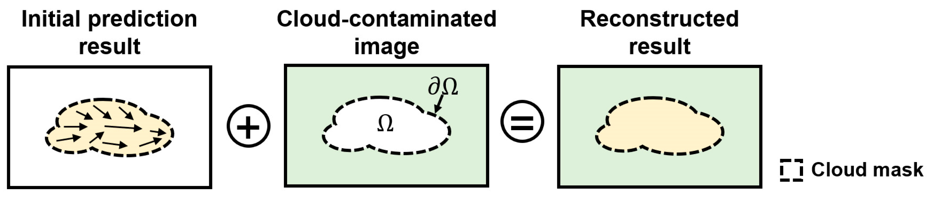
Within the process of cloud removal, the GPR prediction image and the cloud-contaminated image correspond to the source and target images, respectively. Given the cloud mask in the target image () and its boundary (), let be an unknown image reflectance function, defined over the interior of (i.e., target reflectance values within the cloud mask) and let be a known image reflectance function defined outside of in the target image (i.e., reflectance values in non-cloud regions). Poisson blending aims to find the unknown function , which reconstructs reflectance values within without any discontinuity around (Figure 2). To this end, image editing proceeds such that (1) the source image has the same reflectance value on as the target image and (2) the gradient for each pixel over the interior of the source image should preserve the original gradient of the source image. By imposing these constraints, the reconstructed cloud region features a variation in reflectance corresponding to the GPR prediction results and is also consistent with the reflectance of the non-cloud region in the target image around the cloud boundary.

Figure 2.
Poisson blending procedures for seam elimination around the cloud boundary. and represent the interior and boundary of the cloud mask, respectively. Arrows within the cloud mask in the initial prediction result denote the gradient field.
Under the guidance of vector field v defined over the interior of in the source image, Poisson blending is formulated using the following the minimization problem [41]:
where is the gradient operator.
Solving Equation (7) is equivalent to finding the solution of the following Poisson equation with Dirichlet boundary conditions [41]:
where and div are the Laplacian operator and the divergence of a vector field, respectively.
A set of four connected neighbors for the pixel in the target image is usually considered to approximate the differential operators in the discrete image domain. Based on this finite difference approach, a numerical solution of Equation (8) is then obtained by solving a sparse linear system [42].
3. Experiments
3.1. Study Area and Data
Cloud removal experiments were conducted on images of two agricultural sites in Korea, Gimje (Site 1) and Hapcheon (Site 2), as shown in Figure 3. The two sites are major rice and garlic/onion production regions in Korea, respectively. Thus, cloud-free image time series are required for crop monitoring. The transplanting and harvesting periods for rice grown at Site 1 are in May and October, respectively. Garlic and onions at Site 2 have the highest vegetative vitality from late April to early May. Harvesting begins in late May. The total areas of the two sites are 2500 ha and 676 ha, respectively.
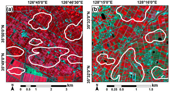
Figure 3.
False color composites of Sentinel-2 images in two sites (near infrared-red-green bands as R-G-B): (a) Sentinel-2 imagery on 20 August 2021 at the Gimje site (Site 1); (b) Sentinel-2 imagery on 14 April 2021 at the Hapcheon site (Site 2). White polygons shown in the Sentinel-2 imagery represent synthetic cloud masks.
In this study, Sentinel-2 images were used as input for cloud removal experiments (Figure 3). The Sentinel-2 images have often been utilized for crop monitoring because the combined constellation of Sentinel-2A and -2B satellites provides images every five days. Out of the twelve spectral bands of the level-2A bottom-of-atmosphere (BOA) products [43], the reflectance values of four spectral bands, including green, red, red-edge, and near infrared (NIR) bands, were considered for cloud removal experiments because they have frequently been used to calculate several vegetation indices for crop monitoring (Table 1). The red-edge 1 band with a spatial resolution of 20 m was resampled to 10 m using bilinear resampling to match the spatial resolution of all the spectral bands to 10 m. Among the cloud-free Sentinel-2 images acquired in 2021 for each site, 20 August and 14 April were experimentally selected as the prediction dates for Site 1 and Site 2, respectively, because vegetative vitality was high at both sites on those dates. Based on preliminary tests, reference dates showing a high correlation with the prediction dates were selected for the two sites (26 July and 10 March, respectively).

Table 1.
Summary of Sentinel-2 images used for the experiments (NIR: near infrared).
3.2. Experimental Design
The synthetic cloud masks shown in Figure 3 were first generated in cloud-free Sentinel-2 imagery at to evaluate quantitative prediction performance within the cloud removal experiment. The cloud masks in this study included a large amount of clouds composed of various types of land cover. The cloud type was assumed to be thick clouds that block signals from the land surface, and the cloud masks include both thick clouds and shadows. When clouds are widely distributed over the study area, they may be located at the edge of the image. In this case, is not available when interpolating reflectance values around edge pixels. To solve this limitation, the GPR prediction values of the edge pixels were assumed to be when clouds are located at the edge of the image. Based on this assumption, GPR prediction values were first assigned to the edge of the cloud masks that actually belonged to clouds. Poisson blending was then applied by regarding GPR prediction values as non-cloud values at . In considering this case, some cloud masks were particularly placed at the edges of the image, as shown in Figure 3. Finally, the cloud masks, consisting of 1 for the cloud region and 0 for the non-cloud region, were prepared and utilized as input for the cloud removal experiment. The actual reflectance values for each spectral band of the cloud region were used to compute quantitative evaluation metrics. The cloud masks occupy approximately 26% of the study area at both sites.
Based on our previous studies [27,38] and computational efficiency, 1% of the non-cloud pixels in the study area, 2500 and 676 for Site 1 and Site 2, respectively, were randomly extracted and then used as training samples for GPR model training.
The prediction performance of the proposed cloud removal method was compared with that of two existing cloud removal methods, including modified NSPI (MNSPI) [29] and geostatistical NSPI (GNSPI) [44]. The two methods were selected because they are hybrid methods, like the proposed method, and their source code is publicly available [45]. MNSPI reconstructs persistent missing regions through the weighted combination of similar pixels based on spectral and spatial distances from auxiliary spatial information [29]. In GNSPI, missing information is predicted by combining regression-based temporal information with kriging of residuals [44]. GNSPI utilizes multi-temporal images to extract spectrally similar neighboring pixels. For a fair comparison with MNSPI and the proposed method using a single reference image, this study utilized a single reference image to implement GNSPI. The common parameters for MNSPI and GNSPI are the number of land cover types and the size of the moving window for extracting neighboring pixels, which were set to 7 and 5, respectively. In addition, the GPR prediction was compared with the final prediction to investigate the effect of Poisson blending-based discontinuity elimination.
All cloud removal methods were applied to each of the four spectral bands of the Sentinel-2 image, and prediction results for each spectral band were compared quantitatively and qualitatively. The four spectral bands are often used to calculated the vegetation index, which is the essential information source for crop monitoring. Thus, to highlight the importance of cloud removal for crop monitoring, the reflectance values of the four spectral bands were utilized to calculate the vegetation index. The predictive performance of different cloud removal methods was then evaluated by comparing the accuracy of the calculated vegetation index. This study considered three vegetation indices that can be calculated from the four spectral bands: (1) normalized difference vegetation index (NDVI), (2) normalized difference red-edge (NDRE), and (3) normalized difference water index (NDWI):
where denotes the reflectance of a specific spectral band.
Two evaluation metrics, the relative root mean square error (rRMSE) and structural similarity index measure (SSIM), were used to measure predictive performance. Since each spectral band has different ranges of spectral reflectance, rRMSE was considered for a relative comparison. SSIMs measure spatial similarity by comparing structural information between actual and predicted reflectance values in cloud regions [46]. Smaller rRMSE values indicate higher prediction accuracy. On the other hand, the closer the SSIM value is to one, the better the structural similarity.
Given actual reflectance values () and predicted values () for a specific spectral band in cloud regions consisting of M pixels (), rRMSE and SSIM are calculated as follows:
where and are the mean and variance values for the actual reflectance values, respectively. are are the mean and variance values for the predicted reflectance values, respectively. denotes the covariance between actual and predicted reflectance values. and are two constraint constants.
The Scikit-learn library [47] and the Python code of Poisson image editing [48] were utilized to implement GPR and Poisson blending, respectively. All data processing, including weighted predictions and evaluation metrics computation, was implemented using Python programming.
4. Results
4.1. Reflectance Prediction
Table 2 lists the quantitative evaluation results for each spectral band. The proposed method achieved the best predictive performance at both sites. MNSPI showed a worse predictive performance for all spectral bands at both sites, except GNSPI which was worse for the red band at Site 1. Significant improvements in rRMSE compared with the worst method were found in the red-edge and NIR bands at both sites. The improvements in the rRMSE of the proposed method over that of MNSPI were 19.27% and 13.34%, respectively, for the red-edge and NIR bands at Site 1. The proposed method also increased the rRMSE by 11.19% and 12.54% for the red-edge and NIR bands, respectively, at Site 2, compared to MNSPI. The superiority of the proposed method was also shown in the SSIM, except for the green band at Site 2. The maximum relative improvement in SSIM was obtained for the red-edge and NIR bands. These quantitative comparison results indicate that the proposed method can effectively capture the structural characteristics and overall quality of the actual reflectance values in cloud regions. The predictive performance of GPR was slightly worse than that of GNSPI, except for the green band at Site 1 and the NIR band at Site 2. However, GPR outperformed MNSPI for all spectral bands.
Table 2.
Band-wise accuracy statistics of different cloud removal methods at the two study sites (rRMSE: relative root mean square error; SSIM: structural similarity index measure; MNSPI: modified neighborhood similar pixel interpolator; GNSPI: geostatistical neighborhood similar pixel interpolator; GPR: Gaussian process regression; NIR: near infrared). The best metric is shown in bold.
When comparing the GPR prediction with the final prediction of the proposed method, Poisson blending increased the rRMSE and SSIM for all spectral bands at both sites. Poisson blending interpolates from the actual value of the non-cloud regions to the inside cloud regions to maintain the spectral pattern. Thus, the proposed method yielded a decrease in rRMSE and an increase in SSIM. Since the GPR predictions achieved better predictive performance in a relative sense, the final prediction obtained after applying Poisson blending demonstrated the best prediction accuracy, confirming the potential of the proposed hybrid method for use in cloud removal.
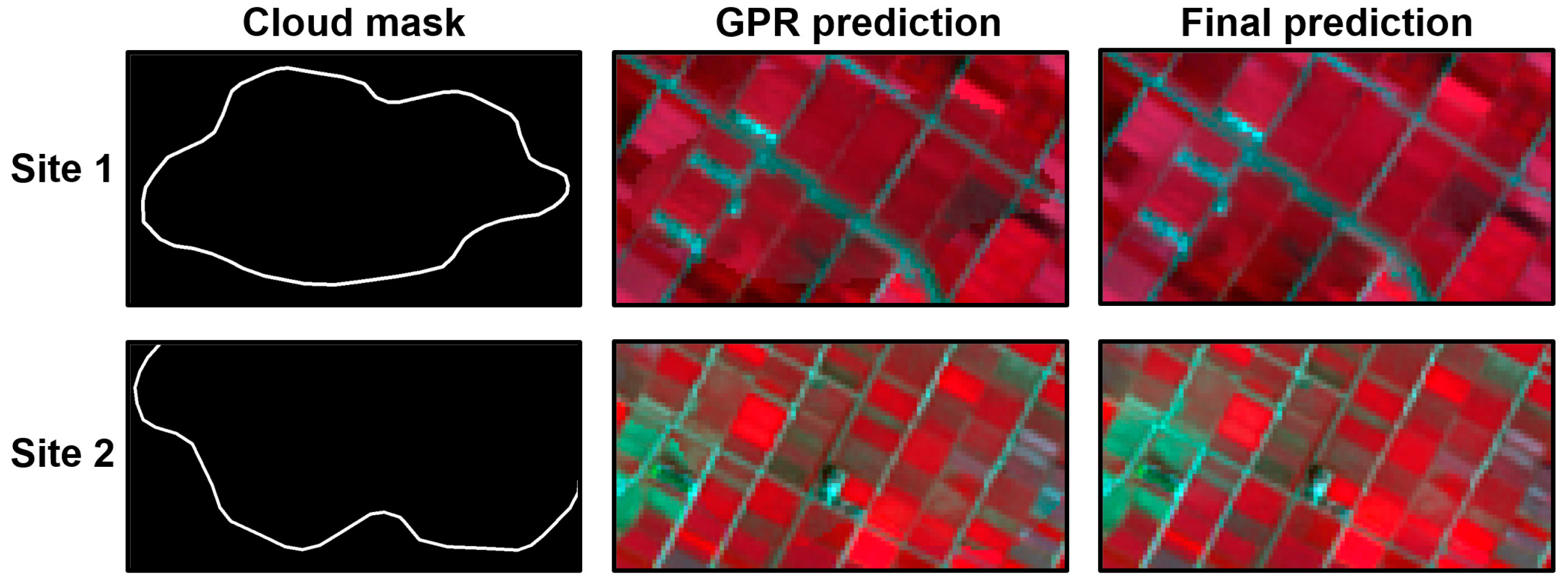
Figure 4 shows the zoomed subareas around the cloud masks. Compared to the GPR predictions, the final prediction results clearly showed natural variations in reflectance around the cloud outline upon visual inspection, demonstrating the necessity of discontinuity elimination via Poisson blending after generating the GPR prediction.
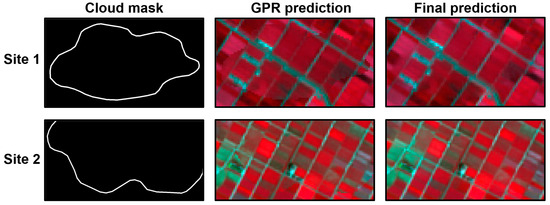
Figure 4.
Visual comparisons between GPR and final predictions in subareas at the two study sites.
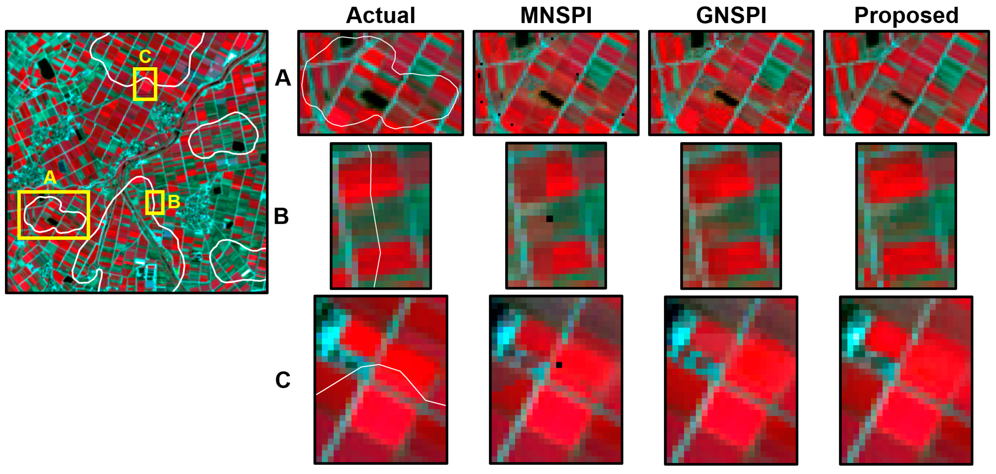
The effect of seam removal via Poisson blending is clearly revealed upon comparison with MNSPI and GNSPI at both sites (Figure 5 and Figure 6). The MNSPI prediction shows noticeable differences in spectral patterns between cloud and non-cloud regions around cloud outlines at Site 1 (Figure 5). Due to the low reflectance in the NIR band in most cloud regions, the image appears relatively dark, and there are also outliers at some cloud boundaries. Discontinuities near cloud outlines are somewhat less pronounced in the GNSPI prediction than in the MNSPI prediction, but spectral distortions still exist inside the cloud region. In addition, the spectral reflectance of some pixels near the cloud boundary is low, resulting in irregular spectral patterns within the crop parcel. In contrast, the proposed method restored the reflectance of the cloud region so that it was similar to the actual reflectance. Spectral discontinuity around the cloud outline is alleviated, and the reflectance inside the crop parcel is distributed evenly and continuously.
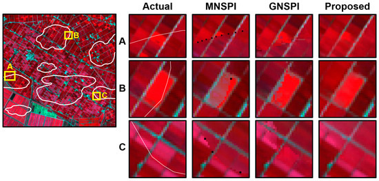
Figure 5.
Visual comparison of three prediction results with a false color composite of the actual imagery (NIR-red-green bands as R-G-B) in three subareas at Site 1. The white line marked in the image represents the synthetic cloud mask, the yellow boxes represent the three subareas, and the black dots indicate very low reflectance values.
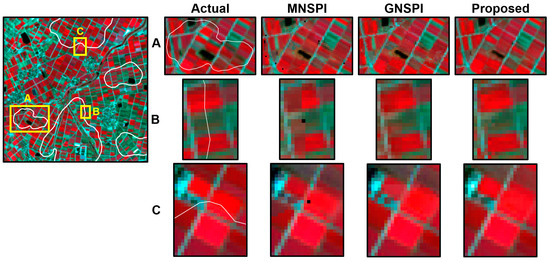
Figure 6.
Visual comparison of three prediction results with a false color composite of the actual imagery (NIR-red-green bands as R-G-B) in three subareas at Site 2. The white line marked in the image represents the synthetic cloud mask, the yellow boxes represent the three subareas, and the black dots indicate very low reflectance values.
Similar to Site 1, the reconstruction results of the proposed method were also visually better than those of the two existing methods at Site 2 (Figure 6). As shown in subarea A, MNSPI prediction showed, in relative terms, the most prominent discontinuity, and GNSPI also showed blurred boundaries in some crop parcels. The two existing methods failed to capture the structural characteristics of the relatively smaller crop parcels than at Site 1.
4.2. Vegetation Indices Prediction
The quantitative evaluation results of the vegetation index predictions are summarized in Table 3. The mean of the actual NDWI values at both sites was negative, so the absolute mean value was used to calculate the rRMSE of the NDWI predictions.
Table 3.
Accuracy statistics of different cloud removal methods for three vegetation indices prediction at the two study sites (VI: vegetation index; NDVI: normalized difference vegetation index; NDRE: normalized difference red-edge; NDWI: normalized difference water index). The best metric is shown in bold.
As expected, the proposed method yielded the best predictive performance for the three vegetation indices with the lowest rRMSE and the largest SSIM. Like the reflectance predictions, MNSPI showed the worst prediction accuracy and structural similarity at both sites, except for the NDVI prediction of GNSPI at Site 1. The worst rRMSE of GNSPI in NDVI prediction at Site 1 is attributed to its worse accuracy in red band prediction. The predictive performance of the NDWI prediction regarding GPR was better than that of MNSPI and GNSPI at both sites. The maximum increase in the rRMSE of the proposed method, compared with the worst predictor, was observed in its NDRE prediction (13.25% at Site 1 and 10.69% at Site 2) followed by the NDWI prediction. The reflectance values predicted in cloud regions are directly fed into the calculation of the vegetation index. Thus, the quality of the computed vegetation index is subject to errors in the reflectance predictions. As two spectral bands are utilized to calculate the vegetation index, the errors of each spectral band together affect predictive performance. Although the proposed method yielded the smallest rRMSE in NIR band prediction, the relatively large errors in red band prediction resulted in a smaller improvement in the rRMSE of the NDVI prediction. Meanwhile, the smallest rRMSE in the prediction of the red-edge and NIR bands of the proposed method led to the most significant improvement in the rRMSE of the NDRE prediction. For SSIM, the proposed method showed the best structural similarity for all three vegetation indices at both sites. In particular, the GPR prediction achieved the second-largest structural similarity.
5. Discussion
5.1. Contribution of the Study
The superiority of our method in this study was attributed to both GPR-based predictions with high quality and seam removal via Poisson blending. It should be noted that the purpose of Poisson blending employed in the second stage is not to improve prediction accuracy. Instead, Poisson blending is used to remove seams and enhance naturalness in reflectance around cloud outlines. Thus, a substantial improvement in prediction accuracy cannot always be expected when applying Poisson blending alone. Therefore, initial predictions with reasonably high accuracy should be used as input for Poisson blending. Compared to random forest regression applied in previous studies [26,49], GPR showed a better prediction performance in cloud removal [38]. In addition, the potential of GPR was demonstrated in many existing gap-filling studies [35,36]. Based on previous studies, GPR was selected in this study to generate initial predictions for cloud removal. Consequently, although the temporal relationship between the reference and prediction dates was purely modeled and used for prediction in GPR, the performance of the GPR prediction was compatible with or better than that of MNSPI and GNSPI, which take a spatio-temporal hybrid approach. One of the advantages of GPR over other machine learning-based regression models is the availability of the predictive uncertainty information (i.e., predictive variance) along with predictions [39]. To date, however, few studies have applied predictive uncertainty information for interpretation or value-added product generation. In this study, predictive standard deviation was combined with predictive value to give less weight to uncertain predictions. Since the gradient, rather than the reflectance value itself, is modeled within the process of Poisson blending, weighted prediction based on two strategies was utilized as the input for Poisson blending.
In their application of Poisson blending to cloud removal, existing hybrid approaches first blend two images acquired on different dates by substituting the non-cloud pixels in the reference image for the cloud region in the prediction image [30,31]. Taking such a cut-and-paste approach, Poisson blending may fail to alleviate the discontinuity around cloud outlines when significant changes occur between reference and prediction dates. To mitigate this limitation, the proposed method replaced cloud regions with GPR predictions based on quantitative relationships between reference and prediction dates and predictive uncertainty. By enhancing naturalness through Poisson blending, prediction results could exhibit more significant structural coherence and maintain the overall spectral patterns in the cloud regions, as confirmed by the smallest rRMSE and the highest SSIM in the comparisons at the two cropland sites. The benefits of our method can be further verified through a comparison of the temporal differences in NDVI between reference and prediction dates. The two sites exhibited different temporal relationships between the reference and prediction dates. At Site 1, the average NDVI values for the reference and prediction dates were similar, with values of 0.72 and 0.79, respectively. In contrast, at Site 2, the average NDVI values for the reference and prediction dates were significantly different (0.27 vs. 0.51), indicating a substantial variation in vegetation vitality between the two dates. The predictive performance of the proposed method at Site 2 outperformed that at Site 1, as shown in Table 2. This result confirms the superiority of our method over conventional cut-and-paste approaches, particularly when there are spectral differences between the two dates.
5.2. Future Research Directions
While our method has demonstrated superior predictive performance, additional refinements and potential applications should be included in future work.
In this study, the relationship between the reflectance values of the reference and prediction dates in GPR was modeled independently for each spectral band. The spectral bands considered in this study have a reasonable correlation. Thus, it is worthwhile to evaluate the potential of multi-output Gaussian process regression, which can capture quantitative relationships between correlated multiple inputs [50].
Predictive uncertainty in GPR is epistemic uncertainty that indicates how confident the model is with respect to its predictions [51]. Thus, predictive uncertainty may not always be related directly to prediction errors. As shown in Equation (4), predictive variance is dependent on covariance but independent of data values, like kriging variance in geostatistics [52]. As the covariance depends solely on the location of data points, the predictive variance of any data sets separated by the same distance is the same, regardless of the data values. Prediction errors usually differ in the prediction of actual high and low values. Thus, the predictive uncertainty in GPR provides only indirect information on its measure of prediction accuracy, which is the limitation of the uncertainty-weighted approach in this study. An alternative approach is to quantify the relationship between the error and the predictive uncertainty in the non-cloud region and then convert the GPR variance into error-related values since errors can be calculated in the non-cloud region.
Recently, several studies have applied cloud removal to high spatial resolution satellite images, such as PlanetScope and WordView images, using deep learning and object-based information [53,54]. Our cloud removal method can be applied to cloud removal from high spatial resolution imagery without the need for further modification since GPR-based regression modeling and Poisson blending are independent of the spatial resolution of the input imagery. However, it is worth noting that high spatial resolution imagery often exhibits more spectral variations and irregular shapes in surface objects compared to low spatial resolution imagery. These differences in spatial structures and land-cover types between cloud and non-cloud regions may affect the prediction results of our method. Therefore, future work should include extensive experiments using high spatial resolution imagery.
The dense image time series generated via cloud removal can act as essential information sources for environmental monitoring, as well as cropland monitoring. For example, the characterization and classification of forest types often requires a series of multi-spectral remote sensing images to capture phenological changes in the forest, like crop monitoring and classification. However, the occurrence of cloud-contaminated images may degrade predictive performance [55]. Thus, optical images reconstructed by cloud removal can be effectively employed for the multi-temporal analysis of forests.
With regard to image time series construction, cloud removal can be combined with other approaches. For example, cloud removal may be employed as a preprocessing step in spatio-temporal image fusion for generating fine spatial and temporal resolution imagery [56]. Spatio-temporal image fusion requires both fine temporal resolution but coarse spatial resolution imagery and coarse temporal resolution but fine spatial resolution imagery. Images contaminated by clouds cannot be used as input for spatio-temporal image fusion. Recently, Tange et al. [57] utilized gap-filled images as input to generate all-sky MODIS land surface temperature. Similarly, the cloud removal method proposed in this work can be applied to reconstruct cloud images and combined with a spatio-temporal image fusion method specifically designed for small-scale cropland monitoring [58]. The benefits of our cloud removal method for the spatio-temporal fusion of vegetation indices will be evaluated in future work.
6. Conclusions
The presence of cloud contamination in optical remote sensing imagery poses a significant challenge to cropland monitoring using remote sensing image time series. To address limitations in the usability of cloud-free images, this study presented a two-stage hybrid cloud removal method. Our cloud removal method is a hybrid approach leveraging the advantages of temporal (GPR) and spatial (Poisson blending) methods. The method begins with the generation of regression-based predictions, followed by discontinuity elimination through Poisson blending. Since the quality of input imagery greatly affects the effectiveness of Poisson blending, GPR was employed as the primary regression model due to its superior predictive capability in cloud removal and the availability of predictive uncertainty information. Cloud removal experiments using Sentinel-2 images at two cropland sites demonstrated the effectiveness of our method. The results from our method exhibited reduced spectral discontinuities around cloud outlines and fewer spectral distortions within cloud regions. In comparative evaluations with two existing hybrid methods, our method outperformed them both in terms of rRMSE and SSIM. Moreover, our method was also able to reconstruct vegetation index values within cloud regions, achieving the highest accuracy and structural similarity. These findings confirm that our method can be effectively applied to the construction of cloud-free optical image time series for crop monitoring and thematic mapping.
Author Contributions
Conceptualization, S.P. and N.-W.P.; methodology, S.P. and N.-W.P.; formal analysis, S.P.; data curation, N.-W.P.; writing—original draft preparation, S.P.; writing—review and editing, N.-W.P.; supervision, N.-W.P. All authors have read and agreed to the published version of the manuscript.
Funding
This work was supported in part by the National Research Foundation of Korea (NRF) grant funded by the Korean government (MSIT) (No. NRF-2022R1F1A1069221) and in part by the “Cooperative Research Program for Agriculture Science and Technology Development (Project No. PJ01478703)” Rural Development Administration, Republic of Korea.
Data Availability Statement
The Sentinel-2 images are made publicly available by the European Space Agency via the Copernicus Open Access Hub at https://scihub.copernicus.eu (accessed on 15 August 2023).
Acknowledgments
The authors thank the anonymous reviewers for their constructive comments on the manuscript.
Conflicts of Interest
The authors declare no conflict of interest.
References
- Kazemi Garajeh, M.; Salmani, B.; Zare Naghadehi, S.; Valipoori Goodarzi, H.; Khasraei, A. An integrated approach of remote sensing and geospatial analysis for modeling and predicting the impacts of climate change on food security. Sci. Rep. 2023, 13, 1057. [Google Scholar] [CrossRef]
- Karthikeyan, L.; Chawla, I.; Mishra, A.K. A review of remote sensing applications in agriculture for food security: Crop growth and yield, irrigation, and crop losses. J. Hydrol. 2020, 586, 124905. [Google Scholar] [CrossRef]
- Weiss, M.; Jacob, F.; Duveiller, G. Remote sensing for agricultural applications: A meta-review. Remote Sens. Environ. 2020, 236, 111402. [Google Scholar] [CrossRef]
- Boryan, C.; Yang, Z.; Mueller, R.; Craig, M. Monitoring US agriculture: The US department of agriculture, national statistics service, cropland data layer program. Geocarto Int. 2011, 26, 341–358. [Google Scholar] [CrossRef]
- Orynbaikyzy, A.; Gessner, U.; Conrad, C. Crop type classification using a combination of optical and radar remote sensing data: A review. Int. J. Remote Sens. 2019, 40, 6553–6595. [Google Scholar] [CrossRef]
- Muruganantham, P.; Wibowo, S.; Grandhi, S.; Samrat, N.H.; Islam, N. A systematic literature review on crop yield prediction with deep learning and remote sensing. Remote Sens. 2022, 14, 1990. [Google Scholar] [CrossRef]
- Joshi, A.; Pradhan, B.; Gite, S.; Chakraborty, S. Remote-sensing data and deep-learning techniques in crop mapping and yield prediction: A systematic review. Remote Sens. 2023, 15, 2014. [Google Scholar] [CrossRef]
- Na, S.-I.; Hong, S.-Y.; Ahn, H.-Y.; Park, C.-W.; So, K.-H.; Lee, K.-D. Detrending crop yield data for improving MODIS NDVI and meteorological data based rice yield estimation model. Korean J. Remote Sens. 2021, 37, 199–209, (In Korean with English Abstract). [Google Scholar]
- Main-Knorn, M.; Pflug, B.; Louis, J.; Debaecker, V.; Müller-Wilm, U.; Gascon, F. Sen2Cor for Sentinel-2. In Proceedings of the International Society for Optics and Photonics, Warsaw, Poland, 11–14 September 2017; Volume 10427, p. 1042704. [Google Scholar]
- Hagolle, O.; Huc, M.; Desjardins, C.; Auer, S.; Richter, R. MAJA ATBD—Algorithm Theoretical Basis Document; CNES-DLR Report MAJA-TN-WP2-030 V1.0 2017/Dec/07; Zenodo: Meyrin, Switzerland, 2017. [Google Scholar]
- Magno, R.; Rocchi, L.; Dainelli, R.; Matese, A.; Di Gennaro, S.F.; Chen, C.-F.; Son, N.-T.; Toscano, P. AgroShadow: A new Sentinel-2 cloud shadow detection tool for precision agriculture. Remote Sens. 2021, 13, 1219. [Google Scholar] [CrossRef]
- Shen, H.; Li, X.; Cheng, Q.; Zeng, C.; Yang, G.; Li, H.; Zhang, L. Missing information reconstruction of remote sensing data: A technical review. IEEE Geosci. Remote Sens. Mag. 2015, 3, 61–85. [Google Scholar] [CrossRef]
- Wang, Q.; Tang, Y.; Ge, Y.; Xie, H.; Tong, X.; Atkinson, P.M. A comprehensive review of spatial-temporal-spectral information reconstruction techniques. Sci. Remote Sens. 2023, 8, 100102. [Google Scholar] [CrossRef]
- Zhang, Q.; Yuan, Q.; Li, J.; Li, Z.; Shen, H.; Zhang, L. Thick cloud and cloud shadow removal in multitemporal imagery using progressively spatio-temporal patch group deep learning. ISPRS J. Photogramm. Remote Sens. 2020, 162, 148–160. [Google Scholar] [CrossRef]
- Duan, C.; Pan, J.; Li, R. Thick cloud removal of remote sensing images using temporal smoothness and sparsity regularized tensor optimization. Remote Sens. 2020, 12, 3446. [Google Scholar] [CrossRef]
- Darbaghshahi, F.N.; Mohammadi, M.R.; Soryani, M. Cloud removal in remote sensing images using generative adversarial networks and SAR-to-optical image translation. IEEE Trans. Geosci. Remote Sens. 2022, 60, 415309. [Google Scholar] [CrossRef]
- Zhang, C.; Li, W.; Travis, D.J. Restoration of clouded pixels in multispectral remotely sensed imagery with cokriging. Int. J. Remote Sens. 2009, 30, 2173–2195. [Google Scholar] [CrossRef]
- Maalouf, A.; Carré, P.; Augereau, B.; Fernandez-Maloigne, C. A Bandelet-based inpainting technique for clouds removal from remotely sensed images. IEEE Trans. Geosci. Remote Sens. 2009, 47, 2363–2371. [Google Scholar] [CrossRef]
- Criminisi, A.; Pérez, P.; Toyama, K. Region filling and object removal by exemplar-based image inpainting. IEEE Trans. Image Process. 2004, 13, 1200–1212. [Google Scholar] [CrossRef]
- Rakwatin, P.; Takeuchi, W.; Yasuoka, Y. Restoration of Aqua MODIS band 6 using histogram matching and local least squares fitting. IEEE Trans. Geosci. Remote Sens. 2009, 47, 613–627. [Google Scholar] [CrossRef]
- Shen, H.; Zeng, C.; Zhang, L. Recovering reflectance of AQUA MODIS band 6 based on within-class local fitting. IEEE J. Sel. Top. Appl. Earth Obs. Remote Sens. 2011, 4, 185–192. [Google Scholar] [CrossRef]
- Li, X.; Shen, H.; Zhang, L.; Zhang, H.; Yuan, Q. Dead pixel completion of aqua MODIS band 6 using a robust M-estimator multiregression. IEEE Geosci. Remote Sens. Lett. 2014, 11, 768–772. [Google Scholar]
- Helmer, E.H.; Ruefenacht, B. Cloud-free satellite image mosaics with regression trees and histogram matching. Photogramm. Eng. Remote Sens. 2005, 71, 1079–1089. [Google Scholar] [CrossRef]
- Chen, B.; Huang, B.; Chen, L.; Xu, B. Spatially and temporally weighted regression: A novel method to produce continuous cloud-free Landsat imagery. IEEE Trans. Geosci. Remote Sens. 2016, 55, 27–37. [Google Scholar] [CrossRef]
- Li, X.; Shen, H.; Zhang, L.; Zhang, H.; Yuan, Q.; Yang, G. Recovering quantitative remote sensing products contaminated by thick clouds and shadows using multitemporal dictionary learning. IEEE Trans. Geosci. Remote Sens. 2014, 52, 7086–7098. [Google Scholar]
- Tahsin, S.; Medeiros, S.C.; Hooshyar, M.; Singh, A. Optical cloud pixel recovery via machine learning. Remote Sens. 2017, 9, 527. [Google Scholar] [CrossRef]
- Park, S.; Park, N.-W. Cloud removal using Gaussian process regression for optical image reconstruction. Korean J. Remote Sens. 2022, 38, 327–341. [Google Scholar]
- Chen, J.; Zhu, X.; Vogelmann, J.E.; Gao, F.; Jin, S. A simple and effective method for filling gaps in Landsat ETM+ SLC-off images. Remote Sens. Environ. 2011, 115, 1053–1064. [Google Scholar] [CrossRef]
- Zhu, X.; Gao, F.; Liu, D.; Chen, J. A modified neighborhood similar pixel interpolator approach for removing thick clouds in Landsat images. IEEE Geosci. Remote Sens. Lett. 2011, 9, 521–525. [Google Scholar] [CrossRef]
- Lin, C.H.; Tsai, P.H.; Lai, K.H.; Chen, J.Y. Cloud removal from multitemporal satellite images using information cloning. IEEE Trans. Geosci. Remote Sens. 2012, 51, 232–241. [Google Scholar] [CrossRef]
- Hu, C.; Huo, L.Z.; Zhang, Z.; Tang, P. Multi-temporal Landsat data automatic cloud removal using Poisson blending. IEEE Access 2020, 8, 46151–46161. [Google Scholar] [CrossRef]
- Camps-Valls, G.; Verrelst, J.; Munoz-Mari, J.; Laparra, V.; Mateo-Jimenez, F.; Gomez-Dans, J. A survey on Gaussian processes for earth-observation data analysis: A comprehensive investigation. IEEE Geosci. Remote Sens. Mag. 2016, 4, 58–78. [Google Scholar] [CrossRef]
- Verrelst, J.; Alonso, L.; Camps-Valls, G.; Delegido, J.; Moreno, J. Retrieval of vegetation biophysical parameters using Gaussian process techniques. IEEE Trans. Geosci. Remote Sens. 2012, 50, 1832–1843. [Google Scholar] [CrossRef]
- Mateo-Sanchis, A.; Muñoz-Marí, J.; Pérez-Suay, A.; Camps-Valls, G. Warped Gaussian processes in remote sensing parameter estimation and causal inference. IEEE Geosci. Remote Sens. Lett. 2018, 15, 1647–1651. [Google Scholar] [CrossRef]
- Pipia, L.; Muñoz-Marí, J.; Amin, E.; Belda, S.; Camps-Valls, G.; Verrelst, J. Fusing optical and SAR time series for LAI gap filling with multioutput Gaussian processes. Remote Sens. Environ. 2019, 235, 111452. [Google Scholar] [CrossRef] [PubMed]
- Belda, S.; Pipia, L.; Morcillo-Pallarés, P.; Verrelst, J. Optimizing Gaussian process regression for image time series gap-filling and crop monitoring. Agronomy 2020, 10, 618. [Google Scholar] [CrossRef] [PubMed]
- Pipia, L.; Amin, E.; Belda, S.; Salinero-Delgado, M.; Verrelst, J. Green LAI mapping and cloud gap-filling using Gaussian process regression in Google Earth Engine. Remote Sens. 2021, 13, 403. [Google Scholar] [CrossRef] [PubMed]
- Park, S.; Kwak, G.-H.; Ahn, H.-Y.; Park, N.-W. Performance evaluation of machine learning algorithms for cloud removal of optical imagery: A case study in cropland. Korean J. Remote Sens. 2023, 39, 507–519, (In Korean with English Abstract). [Google Scholar]
- Rasmussen, C.E.; Williams, C.K.I. Gaussian Processes for Machine Learning; The MIT Press: Cambridge, MA, USA, 2006. [Google Scholar]
- Liu, M.; Chowdhary, G.; Da Silva, B.C.; Liu, S.Y.; How, J.P. Gaussian processes for learning and control: A tutorial with examples. IEEE Control Syst. Mag. 2018, 38, 53–86. [Google Scholar] [CrossRef]
- Pérez, P.; Gangnet, M.; Blake, A. Poisson image editing. ACM Trans. Graph. 2003, 22, 577–582. [Google Scholar] [CrossRef]
- Matías Di Martino, J.; Facciolo, G.; Meinhardt-Llopis, E. Poisson image editing. Image Process. Line 2016, 6, 300–325. [Google Scholar] [CrossRef]
- ESA. Copernicus Open Access Hub. Available online: https://scihub.copernicus.eu (accessed on 15 August 2023).
- Zhu, X.; Liu, D.; Chen, J. A new geostatistical approach for filling gaps in Landsat ETM+ SLC-off images. Remote Sens. Environ. 2012, 124, 49–60. [Google Scholar] [CrossRef]
- Polyu Remote Sensing Intelligence for Dynamic Earth (Pride). Available online: https://xzhu-lab.github.io/Pride/Open-Source-Code.html (accessed on 4 September 2023).
- Wang, Z.; Bovik, A.C.; Sheikh, H.R.; Simoncelli, E.P. Image quality assessment: From error visibility to structural similarity. IEEE Trans. Image Process. 2004, 13, 600–612. [Google Scholar] [CrossRef] [PubMed]
- Scikit-Learn: GaussianProcessRegressor. Available online: https://scikit-learn.org/stable/modules/generated/sklearn.gaussian_process.GaussianProcessRegressor.html (accessed on 4 September 2023).
- Poisson Image Editing. Available online: https://github.com/willemmanuel/poisson-image-editing (accessed on 4 September 2023).
- Wang, Q.; Wang, L.; Zhu, X.; Ge, Y.; Tong, X.; Atkinson, P.M. Remote sensing image gap filling based on spatial-spectral random forests. Sci. Remote Sens. 2022, 5, 100048. [Google Scholar] [CrossRef]
- Caballero, G.; Pezzola, A.; Winschel, C.; Sanchez Angonova, P.; Casella, A.; Orden, L.; Salinero-Delgado, M.; Reyes-Muñoz, P.; Berger, K.; Delegido, J.; et al. Synergy of Sentinel-1 and Sentinel-2 time series for cloud-free vegetation water content mapping with multi-output Gaussian processes. Remote Sens. 2023, 15, 1822. [Google Scholar] [CrossRef]
- Hoffer, J.G.; Geiger, B.C.; Kern, R. Gaussian process surrogates for modeling uncertainties in a use case of forging superalloys. Appl. Sci. 2022, 12, 1089. [Google Scholar] [CrossRef]
- Goovaerts, P. Geostatistics for Natural Resources Evaluation; Oxford University Press: New York, NY, USA, 1997. [Google Scholar]
- Wang, J.; Lee, C.K.F.; Zhu, X.; Cao, R.; Gu, Y.; Wu, S.; Wu, J. A new object-class based gap-filling method for PlanetScope satellite image time series. Remote Sens. Environ. 2022, 280, 113136. [Google Scholar] [CrossRef]
- Hasan, C.; Horne, R.; Mauw, S.; Mizera, A. Cloud removal from satellite imagery using multispectral edge-filtered conditional generative adversarial networks. Int. J. Remote Sens. 2022, 43, 1881–1893. [Google Scholar] [CrossRef]
- Illarionova, S.; Shadrin, D.; Tregubova, P.; Ignatiev, V.; Efimov, A.; Oseledets, I.; Burnaev, E. A survey of computer vision techniques for forest characterization and carbon monitoring tasks. Remote Sens. 2022, 14, 5861. [Google Scholar] [CrossRef]
- Belgiu, M.; Stein, A. Spatiotemporal image fusion in remote sensing. Remote Sens. 2019, 11, 818. [Google Scholar] [CrossRef]
- Tang, Y.; Wang, Q.; Atkinson, P.M. Filling then spatio-temporal fusion for all-sky MODIS land surface temperature generation. IEEE J. Sel. Top. Appl. Earth Obs. Remote Sens. 2023, 16, 1350–1364. [Google Scholar] [CrossRef]
- Park, S.; Park, N.-W.; Na, S.-I. An object-based weighting approach to spatiotemporal fusion of high spatial resolution satellite images for small-scale cropland monitoring. Agronomy 2022, 12, 2572. [Google Scholar] [CrossRef]


Disclaimer/Publisher’s Note: The statements, opinions and data contained in all publications are solely those of the individual author(s) and contributor(s) and not of MDPI and/or the editor(s). MDPI and/or the editor(s) disclaim responsibility for any injury to people or property resulting from any ideas, methods, instructions or products referred to in the content. |
© 2023 by the authors. Licensee MDPI, Basel, Switzerland. This article is an open access article distributed under the terms and conditions of the Creative Commons Attribution (CC BY) license (https://creativecommons.org/licenses/by/4.0/).