Delineation of Productive Zones in Eastern China Based on Multiple Soil Properties

Abstract

Accurate soil management has long been the focus of research in agroecology. Crop productivity can be enhanced while reducing environmental threats from excessive fertilization by fully comprehending the spatial variability of soil properties and delineating management zones (MZs). A field investigation was carried out at experimental sites outside Hefei City’s administrative districts in China to study the spatial variability of soil properties and the delineation of MZs. A total of 9601 soil samples were collected in the study area. A variety of soil properties were analyzed, including the pH, organic matter, total nitrogen, alkali-hydrolyzable nitrogen, available phosphorus, available potassium, slowly released potassium, available sulfur, available boron, available copper, available zinc, available iron, and available manganese. The coefficient of variation for various soil properties exhibited a wide range, spanning from 12.2% to 100.5%. The geostatistical results show that most soil properties have moderate to strong spatial autocorrelation, and the ordinary kriging method is used to map the distribution of soil properties. The principal component analysis method was used to reduce the dimension of 13 soil properties to 4 principal components, and the fuzzy c-means clustering method was used to delineate MZs. The calculation results of the fuzzy performance index and normalized classification entropy show that the optimum number of MZs is five. In the study area, the western part exhibits the highest soil fertility, primarily attributed to its elevated organic matter content. Additionally, organic matter emerges as a key factor influencing sustainable agricultural production in this region. These results form the basis for soil managing areas outside the administrative districts of Hefei City.

1. Introduction

Soil is a fundamental resource for food production; it is the medium where crops grow. Understanding soil properties and related nutrient dynamics has numerous implications for soil fertility, agricultural productivity, food security, and environmental health [1,2]. The soil properties show high spatial and temporal heterogeneity [3]; hence, a blanket management system along the varying gradients only leads to unreasonable fertilization, wasting resources, and polluting the environment [4].

Site-specific management zones (SSMZs) involve dividing target areas into multiple management zones (MZs) based on soil properties and specific requirements. This approach effectively addresses the spatial variability of soil properties and allows precise fertilization and cultivation management practices [5]. A management zone (MZ) can be considered as a subpartition of larger areas into smaller ones based on soil properties. Hence, an MZ has distinctive properties that distinguish it from other zones, allowing for specific management measures. In hilly terrains, the implementation of SSMZs emerges as an effective strategy for precision farmland management, aiming to maximize crop productivity [6]. Precise soil-property distribution maps can be generated using ordinary kriging interpolation [7].

In geostatistics, the semivariogram parameters enable the analysis of intrinsic and extrinsic factors’ impact on regional variables, the evaluation of the spatial variation characteristics of soil properties [8,9], and the calculation of an appropriate sampling density, all of which contribute to precision in fertilization [10,11]. However, when delineating MZs based on soil properties, there is often a specific correlation between different soil properties that could result in information duplication. Principal component analysis (PCA) can transform the original variables into new mutually independent principal components (PCs). Fuzzy c-means clustering (FCM) is a frequently employed unsupervised clustering method, often applied to delineate soil MZs [12,13]. Many prior studies have utilized PCA and FCM to categorize farmland soil into distinct areas with uniform soil properties, forming the basis for sustainable soil MZs [14,15,16,17]. Recent research in similar domains has tended to focus on smaller areas (1~2000 km²) or involve fewer soil-sampling points (50~500) [6,15,16,17,18,19]. Despite the development of digital mapping research, the prediction error grows when the point density is insufficient and the interval between points is wide [20]. Therefore, this study collected 9601 soil samples from areas outside the administrative districts of Hefei City (9389 km²) and tested 13 soil physicochemical indicators. This study focuses on dividing the study area into MZs with different soil fertility characteristics, and dividing large-scale diverse areas into agricultural production areas that are easy to manage without considering local factors, such as landforms and parent materials, and random factors, such as land-use patterns, to achieve sustainable agricultural production. Therefore, this study did not consider factors such as whether the farmland in the study area is independent, different land-use patterns, and soil texture (existing studies have shown that the main influencing factors of soil texture are the parent material [21]).

The study area encompasses Chaohu Lake in eastern China and is characterized by a high level of agricultural development. Unfortunately, the misuse of fertilizers has resulted in the degradation of the water and soil environment within the Chaohu Lake Basin. The central hypothesis posits that understanding the spatial distribution of soil properties and outlining production management areas holds paramount significance in curbing excessive agricultural chemical fertilizer usage while simultaneously enhancing efficiency in the Chaohu Lake region. Against this backdrop, the primary objectives of this study are twofold: (a) Employing geostatistics, the study aims to comprehensively analyze the spatial variability of soil properties. By utilizing ordinary kriging interpolation, the research endeavors to generate detailed soil fertility maps. These maps will offer valuable insights into the distribution of key soil properties, enabling a nuanced understanding of the local soil conditions. (b) Utilizing PCA and FCM, the study seeks to delineate distinct agricultural production MZs within the Chaohu Lake region. This approach is anticipated to facilitate a more informed and strategic allocation of resources, contributing to sustainable agricultural practices and mitigating the adverse environmental impacts associated with indiscriminate fertilization.

2. Materials and Methods

2.1. Study Area

The study was carried out in Hefei City, located in the eastern part of China in Anhui Province. Hefei is situated between 30°57′ and 32°32′ N latitude and 116°41′ and 117°58′ E longitude. Hefei City encompasses a total area of 11,445 km², with Chaohu Lake covering an area of 784 km² (Figure 1). Hefei experiences a humid climate, with a multiyear average temperature of 15.5 °C. The highest temperatures are typically recorded in late July, with a multiyear average ranging from 27.5 °C to 28.8 °C. On the other hand, the lowest temperatures are usually observed in January, with a multiyear average of 2.1 °C. The average annual sunshine duration is about 2000 h, the maximum annual sunshine duration is 3544.4 h, and the minimum is 1666.2 h. The multiyear average annual precipitation is 940~1000 mm. The soils at the study sites were yellow–brown soil and Paddy soil, and the main crops were rice and wheat. This study specifically spans Feidong County, Feixi County, Chaohu City, Changfeng County, and Lujiang County, focusing on the areas outside the administrative districts of Hefei City and Chaohu Lake. The total area of the study region is 9389 km², with a cultivated land area of 4586 km².

2.2. Soil-Sampling Site Selection and Collection

The soil point layout in the study was initially segmented into sampling units considering land-use patterns, administrative divisions, and the cultivated land area. Subsequently, a combination of the latest high-resolution remote sensing data and Google images was employed for the random placement of points. These points were then adjusted and validated, ultimately culminating in the determination of sampling points through on-site field surveys. A total of 9601 points were assigned in the study area (Figure 1), including Chaohu City (n = 1624), Feidong County (n = 2229), Feixi County (n = 1652), Lujiang County (n = 2119), and Changfeng County (n = 1977). The sampling period was from September to November 2022. Surface samples (0~30 cm) were mixed at 5 points, and excess samples were discarded using the quartering method. The final sampling weight was from 1 to 2 kg. All collected soil samples underwent testing for 13 physicochemical properties. Soil pH was assessed in a 1:2.5 (w/v) soil–water suspension using a pH meter [22], and organic matter (OM) content was determined through potassium dichromate titration. Total nitrogen (TN) in the soil was determined using the Kjeldahl nitrogen-determination method, while alkali-hydrolyzable nitrogen (AN) was determined through alkaline hydrolysis and diffusion. Soil available phosphorus (AP) levels were measured using the Olsen extraction method, employing alkaline sodium bicarbonate as the extractant at a 20:1 ratio. Soil available potassium (AK) and slowly released potassium (SK) were determined using the neutral ammonium acetate extraction method and ammonium acetate extraction method, respectively. Soil available sulfur (S) was measured using the turbidimetric method, and available boron (B) content was determined using the curcumin colorimetric method. Additionally, available copper (Cu), zinc (Zn), iron (Fe), and manganese (Mn) in the soil were extracted using diethylene triamine penta-acetic acid and quantified using an atomic absorption spectrophotometer [23]. All soil samples were tested by Center Testing International Group Co., Ltd., Shenzhen, China.

2.3. Descriptive Statistics

Before performing geostatistical analysis, the 3 times standard deviation method (mean ± 3 times standard deviation) was used to eliminate outliers [24]. Outliers were replaced with the maximum and minimum values within three times the standard deviation to ensure that the number of sample points remained constant. SPSS 22.0 software (IBM, Chicago, IL, USA) was used for the Pearson correlation analysis among the 13 soil properties, and the minimum, maximum, mean, standard deviation (SD), and coefficient of variation (CV) were computed. Origin 2021b software (Origin Lab, Northampton, MA, USA) was utilized to generate a coefficient plot. The skewness and kurtosis of the frequency histogram were used to test whether the data conformed to the normal distribution. Metrics that are not normally distributed can be log-transformed so that their mean is closer to the median, skewness closer to 0, and kurtosis closer to 3.

2.4. Geostatistical Analysis

Geostatistical methods based on semivariograms are commonly used to study the spatial variation characteristics of soil elements, which can indicate the degree of influence of intrinsic and extrinsic factors on regional variables. For the assessment of the spatial distribution pattern of the soil properties, ArcGIS 10.6.1 software (Redlands, CA, USA) was used and semivariograms for each soil property were calculated using Formula (1), as given, where γ(h) is the semivariance when the spatial distance is h; N(h) is the number of sample pairs separated by the lag distance h; Z(x_i + h) and Z(x_i) are the measured values for the spatial locations at x_i + h and x_i, respectively.

$$\gamma \left(\mathrm{h}\right)=\frac{1}{2\mathrm{N}(\mathrm{h})}{{\displaystyle \sum _{\mathrm{i}=1}^{\mathrm{N}\left(\mathrm{h}\right)}\left[\mathrm{Z}\left({\mathrm{x}}_{\mathrm{i}}+\mathrm{h}\right)-\mathrm{Z}\left({\mathrm{x}}_{\mathrm{i}}\right)\right]}}^2$$

(1)

Among the parameters of the semivariogram, the nugget value (C₀) represents the random variation caused by factors such as human activities and sampling and detection errors, the sill value (C₀ + C) is the total spatial variation, and the nugget-based ratio (C₀/(C₀+ C)) is the proportion of extrinsic variation in the total spatial variation. The size of the block basis ratio can measure the degree of spatial autocorrelation, and its range is the theoretical distance of spatial autocorrelation. Spherical, exponential, Gaussian, K-Bessel, J-Bessel, and stable semivariogram models were evaluated. The best-fitting model for each soil nutrient was selected based on the mean and standard mean of the prediction error being close to 0, the smallest root mean square, the standard root mean square being close to 1, and the mean standard error being close to the root mean square. Block ordinary kriging was used to draw a raster distribution map of the soil properties.

2.5. Principal Component Analysis

Principal component analysis is a technique for reducing the dimensionality of multiple variables by a linear combination of original variables. The PCs are independent of each other and replace the original variables well. PCs with eigenvalues ≥ 1 and a total dataset variance ≥ 60% were selected to delineate the MZs [12,25,26]. Origin 2021b software was utilized to generate a scree plot and bi-plot. Maps of the PCA and MZs were generated on 500 m grids.

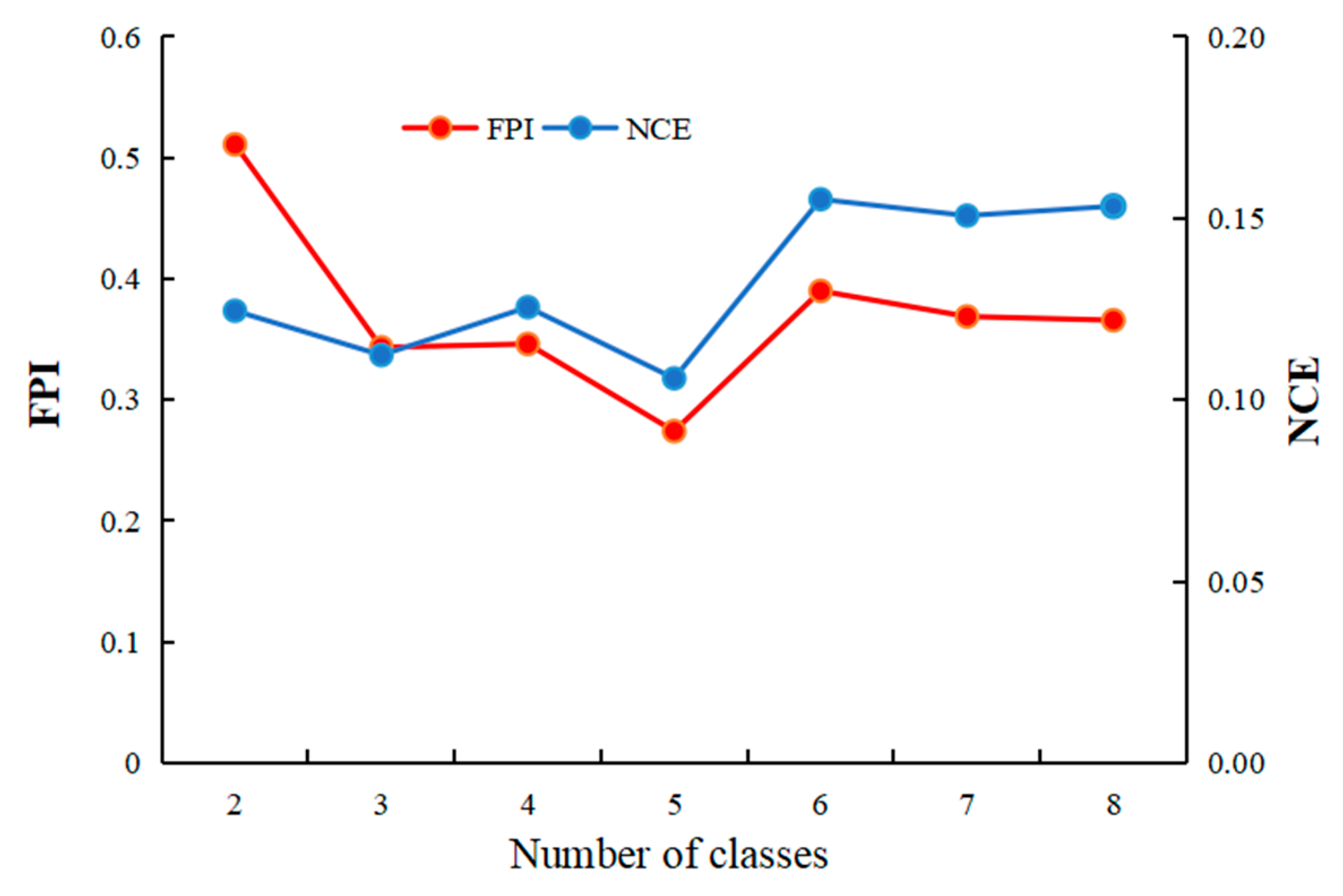
2.6. Fuzzy Cluster Algorithm

The fuzzy c-means clustering method assigns n observations to c categories to obtain clusters with similar characteristics. The cluster centroid and the membership value between each observation and the cluster centroid are continuously calculated through an iterative process. The FCM employs a membership function to perform a weighted summation of squared errors. The objective function is as shown below in Formula (2). The minimum J_FCM corresponds to the best clustering result, where µ_ji is the membership degree of the i-th observation to the j-th cluster; d_ji is the distance from the i-th observation to the cluster center μ_j. In the FCM, the Euclidean distance is used to calculate the distance between the observation value and the cluster center, and the sum of the membership degrees of an observation value to each cluster is 1 [27]. This study completed the FCM method through programming in Matlab R2023a software (The Natick Mall, MA, USA). The FCM options were set to the maximum number of iterations = 300, the stopping criterion of 0.0001, the minimum number of clusters of 2, the maximum number of clusters of 8, and a fuzzy index of 1.5 [13,28].

$$J_{FCM}={{\displaystyle {\sum }_{j=1}^{\mathrm{c}}{\displaystyle {\sum }_{i=1}^n\left({\mu }_{ji}\right)}}}^m{\left(d_{ji}\right)}^2$$

(2)

The fuzzy performance index (FPI) and normalized classification entropy (NCE) were used to determine the optimum number of MZs. The expressions are shown in Formulas (3) and (4), where c is the number of clusters, n is the number of observations, µ_ik is the fuzzy membership degree, and log_a is the natural logarithm. The FPI measurement is the degree of ambiguity produced by a specified number of clusters, with a value ranging from 0 to 1. An FPI value close to 0 indicates that members of different clusters share a little degree, while an FPI value close to 1 indicates that members share a large degree. The NCE is an estimate of the amount of confusion caused by a specified number of classes. The optimum number of MZs is obtained when the FPI and NCE are minimum. Verification with the analysis of variance showed that there is heterogeneity among the different MZs.

$$FPI=1-\frac{c}{c-1}\left[1-\frac{{\displaystyle {\sum }_{i=1}^c{\displaystyle {\sum }_{k=1}^n{\left({\mu }_{ik}\right)}^2}}}{n}\right]$$

(3)

$$NCE=\frac{n}{n-c}\left[-\frac{{\displaystyle {\sum }_{k=1}^n{\displaystyle {\sum }_{i=1}^c{\mu }_{ik}{\log }_a\left({\mu }_{ik}\right)}}}{n}\right]$$

(4)

3. Results

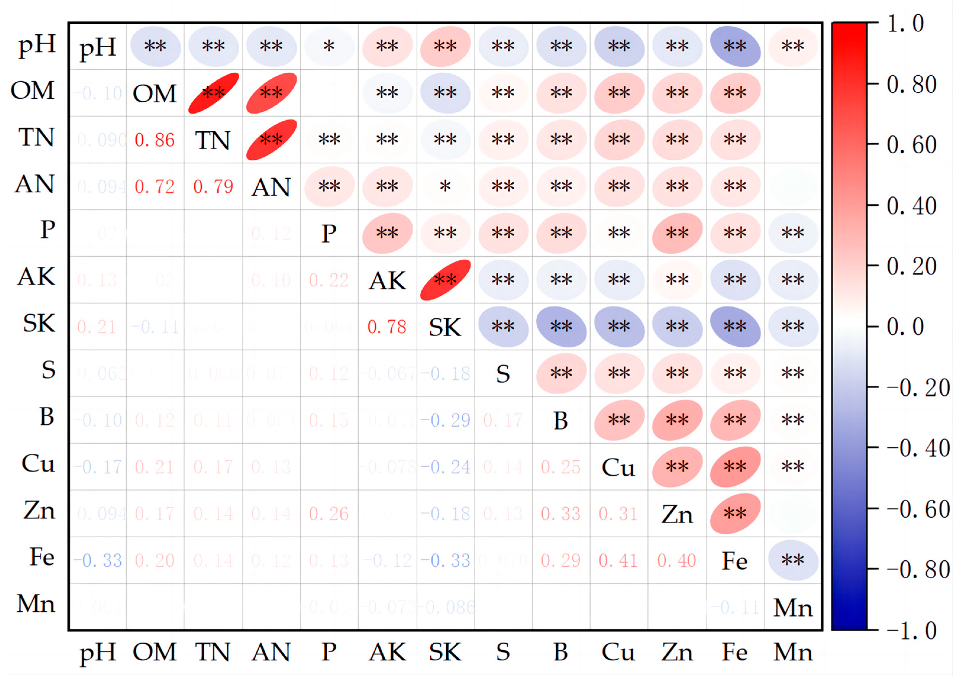
3.1. Descriptive Statistics and Correlation among Soil Properties

The mean, standard deviation, and other descriptive results of the sampling points (9601) for a variety of soil properties in the study area are summarized in

Table 1. Descriptive statistical parameters of the soil properties of the study area.

Soil Properties	Minimum	Maximum	Mean	SD	CV (%)	Distribution Pattern	Skewness	Kurtosis
pH	4.23	8.76	6.06	0.74	12.2	Lognormality	0.06	−0.50
OM (g·kg−1)	1.3	48.7	20.6	7.6	36.8	Normality	0.38	−0.02
TN (g·kg−1)	0.16	2.71	1.19	0.41	34.5	Normality	0.29	−0.06
AN (mg·kg−1)	7	309	124	49	39.8	Normality	0.59	0.27
AP (mg·kg−1)	0.2	148.9	18.3	18.3	100.5	Lognormality	−1.00	2.34
AK (mg·kg−1)	22	594	146	77	53.0	Lognormality	−0.24	0.08
SK (mg·kg−1)	34	1189	334	187	55.9	Lognormality	−0.32	−0.09
S (mg·kg−1)	0.05	148.93	24.55	13.50	55.0	Normality	1.02	5.51
B (mg·kg−1)	0.01	0.80	0.37	0.13	33.8	Normality	0.17	0.54
Cu (mg·kg−1)	0.02	9.17	3.56	1.42	40.0	Normality	0.47	0.14
Zn (mg·kg−1)	0.03	5.51	1.39	0.75	53.8	Normality	0.76	0.33
Fe (mg·kg−1)	0.2	361.5	102.0	81.2	79.6	Normality	0.54	−0.79
Mn (mg·kg−1)	0.6	143.7	41.1	29.0	70.6	Normality	0.61	−0.36

. The results showed that the average soil pH in the study area was 6.06 ± 0.74, ranging from strongly acidic to alkaline. The average soil OM was 20.6 ± 7.6 g kg⁻¹, a key indicator of soil fertility and the source of various soil nutrients. Based on the CV, soil properties can be categorized as low (<10%), medium (10–90%), and high (>90%) [29]. Accordingly, our results indicated that, except for the soil AP, which can be classified as high (100.5%), the remaining soil properties were all under medium, with the soil pH being the smallest value (12.2%). This is consistent with other researchers’ findings that the AP has the highest CV among soil properties, and the pH has the lowest CV [30]. Soil pH exhibits less fluctuation compared to other chemical indicators due to the effective pH-regulating actions of microbial activities. For instance, organic acids or hydrogen ions released by roots can influence the pH in their immediate vicinity [31]. Moreover, mineralization and nitrification processes regulate the soil’s pH and OM, TN, and AN contents [32]. Soil AP is mostly in an adsorbed state in the soil; phosphate, which has weak mobility, quickly accumulates, resulting in a high CV value [33]. The soil OM, TN, AN, S, B, Cu, Zn, Fe, and Mn were all normally distributed. At the same time, the skewness and kurtosis of the pH, AP, AK, and SK were inclined towards the normal distribution following logarithmic transformation (values of the skewness and kurtosis calculated after data transformation are shown in Table 1), thereby providing a basis for the subsequent geostatistical analysis.

The Pearson correlation coefficients between the soil properties in the study area are shown in Figure 2. The results uncovered either a negative or positive correlation among the majority of the 13 soil properties. Notably, the soil pH significantly correlates with all other soil properties; it exhibits a significant positive correlation with the AK, SK, and Mn, while showing a significant negative correlation with the remaining indicators. The correlation with Fe is the strongest, indicating that, with a pH decrease, the concentration of Fe increases. This is because lower pH levels in the soil result in higher iron availability [34]. There is a high correlation between the soil OM, TN, and AN, which has been confirmed by many scholars elsewhere [35,36]. Except for the pH and OM, AP exhibits a significant positive correlation with the other properties. A strong correlation exists between the AK and SK. Despite a modest correlation coefficient, S showed a significant positive correlation with most soil properties. There was a significant positive correlation between any two of B, Cu, Zn, and Fe. Correlations between Mn and other soil properties were mostly weak.

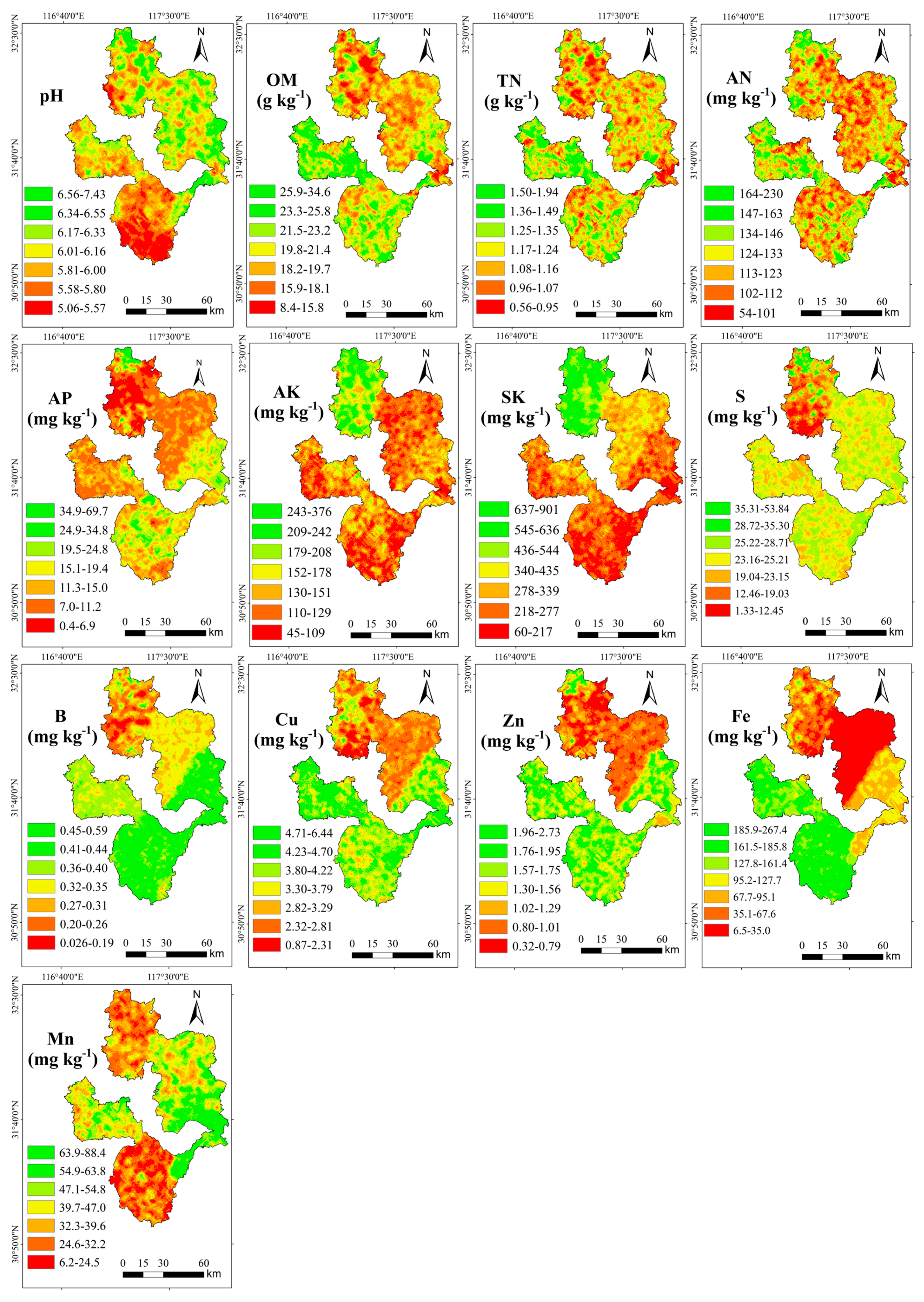
3.2. Geostatistical Analysis

Before calculating the semivariance function, selecting a proper lag size is very important. This study point’s nearest average neighbor (447 m) was calculated and used as the lag size. Ordinary kriging performance was affected by the choice of variogram modeling [37], and the best-fitting model was selected by judging its prediction errors. The best-fitting model and semivariance function parameters for different soil properties are shown in

Table 2. Semivariogram parameters of the soil properties of the study area.

Soil Properties	Model	Nugget	Sill	Nugget/Sill	Range (m)
pH	Spherical	0.012	0.013	0.92	4464
OM (g·kg−1)	Spherical	50.524	52.806	0.96	2926
TN (g·kg−1)	Exponential	0.107	0.163	0.66	535
AN (mg·kg−1)	Gaussian	1187.227	2370.535	0.50	254
AP (mg·kg−1)	Gaussian	0.562	0.604	0.93	2027
AK (mg·kg−1)	Exponential	0.043	0.188	0.23	374
SK (mg·kg−1)	Exponential	0.027	0.198	0.14	458
S (mg·kg−1)	J-Bessel	56.802	77.953	0.73	102
B (mg·kg−1)	J-Bessel	0.009	0.011	0.82	52
Cu (mg·kg−1)	Exponential	0.6	1.613	0.37	399
Zn (mg·kg−1)	J-Bessel	0.325	0.374	0.87	49
Fe (mg·kg−1)	Exponential	1674.865	2585.963	0.65	49
Mn (mg·kg−1)	Gaussian	692.882	726.547	0.95	4225

. The results indicated that the best-fitting model for the soil pH and OM in the study area was spherical; the best-fitting model for the TN, AK, SK, Cu, and Fe was exponential; the best-fitting model for the AN, AP, and Mn was Gaussian. The best-fitting model for the remaining soil properties was J-Bessel. Nugget-to-sill ratios < 0.25, 0.25~0.75, and >0.75 indicate robust, medium, and weak spatial autocorrelation [38]. Soil pH, OM, P, B, Zn, and Mn exhibited strong spatial autocorrelation, indicating that extrinsic factors predominantly influenced the spatial variation. On the other hand, AK and SK displayed weak spatial autocorrelation, implying that intrinsic actors mainly controlled their spatial variation. The remaining soil properties demonstrated moderate spatial autocorrelation, indicating that a combination of intrinsic and extrinsic factors influenced the spatial variation. Similar results from the geostatistical analysis of the soil properties were obtained by Behera [18] and Tripathi [15]. The range denotes the spatial variation range of regional variables, indicating that the soil properties were not affected by intrinsic and extrinsic factors outside the range [39]. The range values of the soil pH, OM, TN, AP, SK, and Mn in the study area were >447 m, while the range values of other soil properties were ≤447 m. Moreover, it was demonstrated that this study’s sample interval could not meet other soil properties other than the soil pH, OM, TN, AP, SK, and Mn [40].

After determining the fitting model, a spatial distribution map was made through ordinary kriging for the 13 properties of the study area, as shown in Figure 3. The spatial difference in the soil pH within the study area was minimal, with the southern part being more acidic and displaying a fragmented distribution pattern. Soil OM, TN, and AN exhibited relatively similar spatial distribution characteristics, with higher values observed in the northeast and lower values in the southwest, often accompanied by distinct patchy patterns. Soil AP demonstrated the most considerable spatial difference, characterized by a noticeable clustering of the high and low values. In general, the AP tends to increase gradually from the northwest to the southeast. Soil AK and SK, owing to their physical and chemical properties, maintained a high degree of spatial uniformity [41,42], with prominent large-scale aggregation in Changfeng County in the north, distinguishing it from other regions. The S exhibited a highly fragmented distribution, particularly in the northern region, displaying substantial spatial differences. Soil B, Cu, Zn, and Fe showed relatively small differences within counties but exhibited significant differences between counties. Notably, Fe displayed the most pronounced variation, generally higher in the north and lower in the south. The spatial distribution of Mn was notably different and fragmented, with lower values observed in both the northern and southern regions, and higher values in the eastern region.

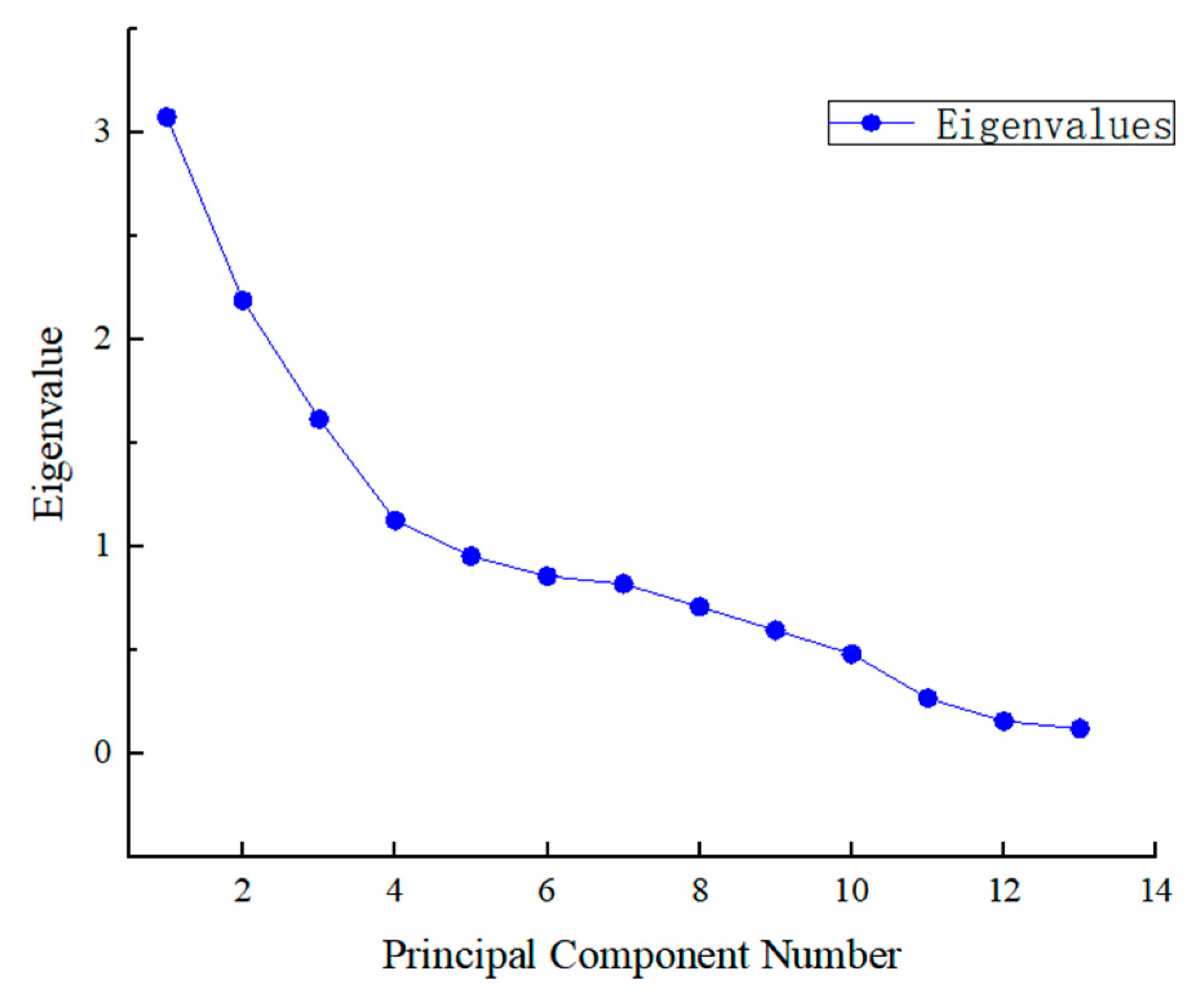
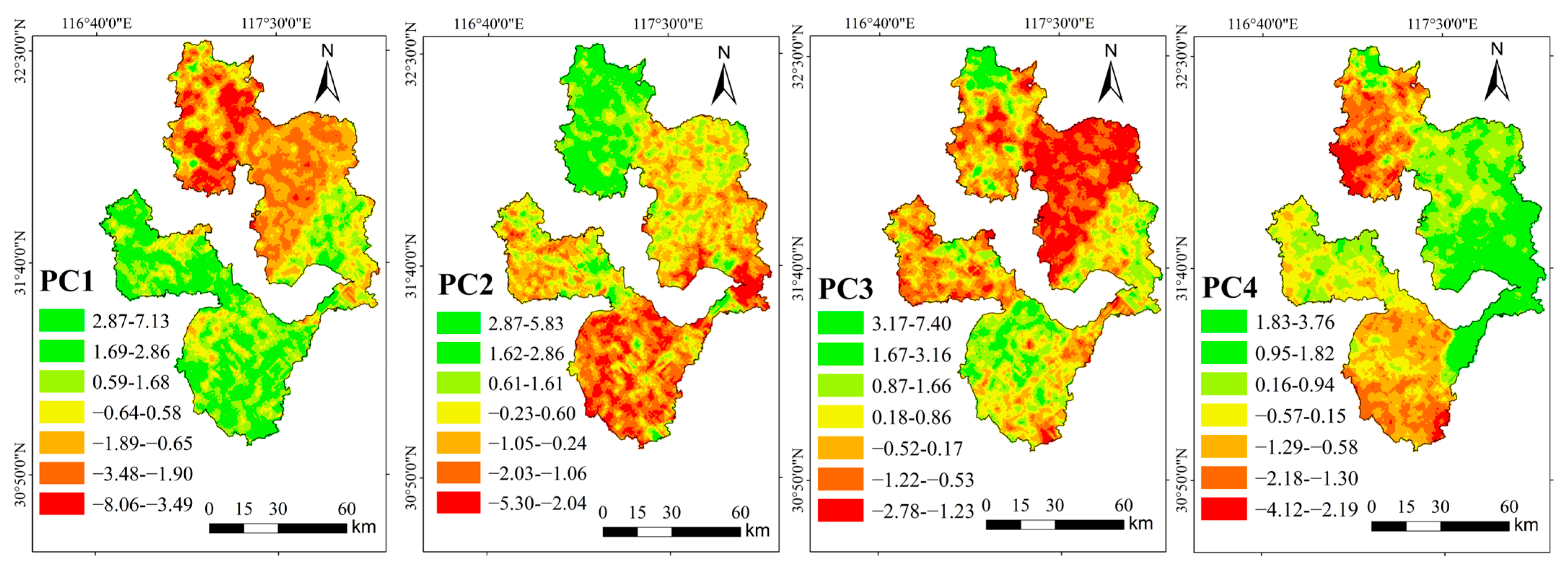
3.3. Principal Component Analysis

A significant correlation existed among the 13 soil properties in this study. The PCA was employed to streamline and summarize the variation within these properties. Consequently,

Table 3. Principal component analysis of the soil properties.

Principal Component	Eigenvalues	Component Loading (%)	Cumulative Loadings (%)
PC1	3.076	23.664	23.664
PC2	2.191	16.853	40.517
PC3	1.618	12.446	52.963
PC4	1.128	8.680	61.643
PC5	0.956	7.350	68.993
PC6	0.860	6.615	75.608
PC7	0.823	6.329	81.938
PC8	0.711	5.469	87.407
PC9	0.599	4.606	92.012
PC10	0.484	3.723	95.735
PC11	0.271	2.082	97.817
PC12	0.160	1.230	99.047
PC13	0.124	0.953	100.000

presents the eigenvalues and cumulative loadings for the 13 PCs derived from the analysis. PCs with eigenvalues surpassing 1 and cumulative loadings exceeding 60% were chosen. By incorporating the Scree plot (Figure 4), the final analysis focuses on the first four principal components, which collectively contribute to 61.6% of the total variability.

The bi-plot (PC1 vs. PC2) facilitates the identification of soil-property priorities and illustrates three primary groupings (Figure 5). Soil TN, AN, and OM constitute the first group, while Cu, Zn, Fe, and B form the second group. The third group comprises AK, SK, and pH.

The loading values for all soil properties for the four PCs are presented in

Table 4. Principal component loading for each variable.

Principal Component	pH	OM	TN	AN	AP	AK	SK	S	B	Cu	Zn	Fe	Mn
PC1	−0.343	0.767	0.744	0.678	0.173	−0.190	−0.426	0.255	0.441	0.524	0.500	0.572	0.004
PC2	0.259	0.454	0.539	0.570	0.073	0.637	0.714	−0.183	−0.318	−0.267	−0.194	−0.368	−0.060
PC3	−0.013	−0.274	−0.257	−0.160	0.623	0.626	0.383	0.134	0.306	0.190	0.504	0.279	−0.211
PC4	0.499	−0.001	0.020	0.020	0.174	−0.022	−0.082	0.443	0.257	−0.038	0.114	−0.336	0.672

. Higher absolute values indicate a greater contribution to the PCs. In the PC1, the OM, TN, and AN made the most substantial contributions, with trace elements, such as B, Cu, Zn, and Fe, also contributing measurable amounts. Soil AK and SK primarily influenced PC2. PC3 saw significant contributions from the AP and AK, while Mn, S, and pH played the most noticeable roles in PC4.

By splitting the study area into fishing-net-like units, 39,125 units measuring 500 m in width and height each were found. The average value of the 13 soil properties on each unit was assigned to the unit. The four PCs were calculated according to Table 3 [43]. The distribution diagrams of the four PCs were generated using ArcGIS 10.6.1 software, as illustrated in Figure 6. The distribution maps of these four PCs exhibited similarities to the spatial distribution maps of the thirteen soil properties to varying degrees; this suggests that the four PCs effectively captured and reflected the spatial distribution characteristics of the thirteen soil properties. Notably, PC1′s spatial distribution closely resembled that of OM, PC2 was highly correlated with SK, PC3 exhibited similarities to AP, and PC4 showed a strong resemblance to Mn.

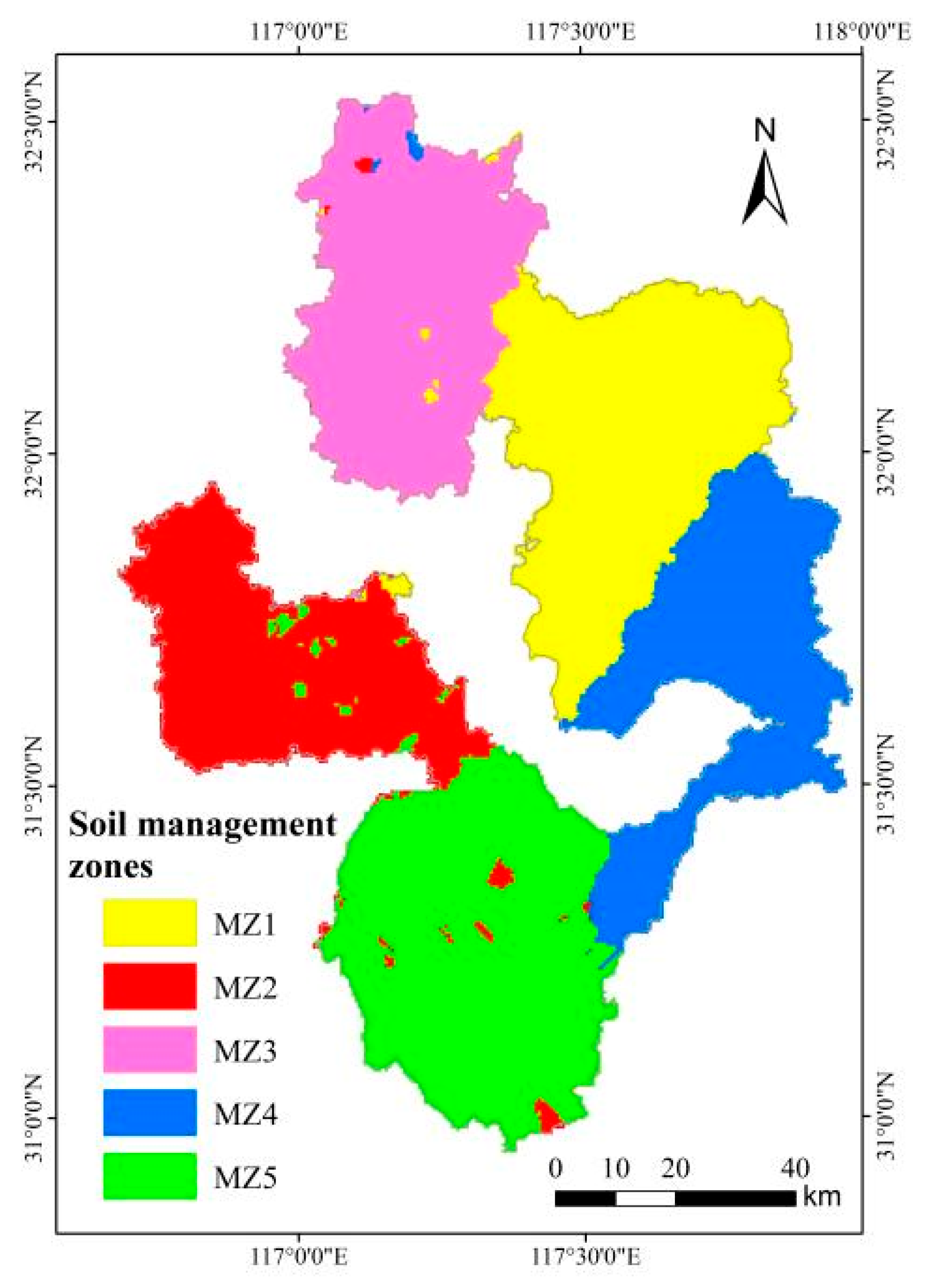
3.4. Delineation and Evaluation of the Management Zones

Selection of the optimum number of MZs is crucial for delineating the MZs. In this study, the scores of the four PCs were imported into Matlab R2023a sotfware, two to eight clusters were selected sequentially, the FCM algorithm was run, and the corresponding FPI and NCE were calculated, as shown in Figure 7. The optimum number of MZs was selected to be five clusters, since FPI and NCE were simultaneously at their lowest at five.

The map of the MZs is shown in Figure 8, in which the results of five cluster classes were drawn using ArcGis10.6 software. The results indicated that MZ1, MZ2, MZ3, MZ4, and MZ5 contained 8901 (22.75%), 6665 (17.04%), 7572 (19.35%), 6774 (17.31%), and 9213 (23.55%) units, respectively.

The spatial outcomes of the five zones were superimposed onto the original 9601 soil-sampling points to verify the zoning results. Variance analysis was conducted to assess the heterogeneity of the 13 soil properties across the different MZs, and the test results are presented in

Table 5. Mean values of the soil properties in the five management zones.

Management Zone	n	pH	OM	TN	AN	AP	AK	SK	S	B	Cu	Zn	Fe	Mn
MZ1	2238	6.21 a	19.1 c	1.16 c	115 d	12.3 d	118 d	328 b	24.73 ab	0.33 c	2.77 e	0.89 c	20.0 e	47.0 b
MZ2	1650	6.03 b	23.6 a	1.31 a	137 a	14.4 c	130 c	272 c	24.31 b	0.37 b	4.36 a	1.70 a	164.1 b	44.2 c
MZ3	1952	6.19 a	18.7 d	1.12 d	129 b	19.5 b	207 a	556 a	20.78 c	0.28 d	2.92 d	1.09 b	64.7 d	31.6 d
MZ4	1634	6.19 a	21.1 b	1.19 b	126 b	20.0 b	137 b	245 d	25.16 a	0.44 a	4.06 b	1.68 a	91.9 c	57.0 a
MZ5	2127	5.69 c	21.0 b	1.18 bc	118 c	21.3 a	130 c	239 d	24.67 ab	0.45 a	3.98 c	1.71 a	182.4 a	28.6 e

Different letters within each column indicate significant difference between the management zones at 0.05 level.

. Most soil properties exhibited significant variations among the different MZs. Cu and Fe, in particular, displayed significant variances among the five MZs, indicating that the zoning outcomes were most effective for Cu and Fe. The spatial heterogeneity of S in the five MZs was relatively weaker. Of the 13 soil properties examined in this study, the distinctions between MZ1, MZ2, and MZ3 and the other MZs were more evident than the differences between MZ4 and MZ5 and the other MZs, which were less noticeable.

4. Discussion

The primary macronutrients—AN, AP, and AK—are crucial factors limiting crop development in the soil [44,45]. The delineation results reveal that the northeastern region of the study area (MZ1) exhibited the lowest average values for the AN, AP, and AK, underscoring the need for appropriate fertilizer input in this zone. To achieve an ideal crop yield, the amount of fertilizer should be increased proportionally in formula fertilization. Assessing the mean soil properties of the MZs, the western part of the study area (MZ2) generally exhibited higher soil fertility, prominently reflected in its elevated soil OM, TN, and other values. This can be attributed to the prevalence of mountains and hills in this area, fostering more plants, whose litter and moist air promote the accumulation of OM and TN [46]. Furthermore, soil OM is a critical source of various nutrients [47] and serves as a key indicator for evaluating soil quality [48,49]. The bi-plot in this study also demonstrates that OM is the most influential factor affecting the sustainable utilization of agriculture in terms of soil properties. The eastern part of the study area (MZ3) showed the lowest levels of OM, emphasizing the necessity to promote practices such as straw return and organic fertilizer application [50,51] in this zone. Examining the soil-property distribution map, it is evident that the soil pH and OM exhibit highly similar spatial distributions, as humic acid decomposed by OM contributes to a reduction in the soil pH [52]. The southern (MZ5) and western (MZ2) parts of the study area displayed the lowest soil pH, suggesting the requirement for soil amendments, such as applying acid soil conditioners [53,54,55] and reducing the use of simple chemical fertilizers [56]. The nugget-to-sill ratios of the AK and SK in the study area were significantly smaller compared to other soil properties, owing to the close relationship between potassium and parent rock minerals. Simultaneously, the high temperature and rainy climate in the mountainous and hilly areas [57] contribute to easier potassium loss. Based on comprehensive soil-property indicators, the soil in the western part of the study area (MZ2) is the most fertile. However, to further improve crop productivity, one should consider other limiting factors beyond soil properties. It is crucial to note that these recommendations are specific to the study area, confined within Hefei City. In crop management and fertilization, various factors—including the local nutrient status, crop varieties, climate, and precipitation—must be considered [58,59,60,61,62,63,64].

This study’s management zone delineation closely matches Hefei City’s administrative divisions. Upon examining the ordinary kriging interpolation results of the 13 soil properties within the study area and the distribution map of PCs, it becomes evident that the reason for this outcome lies in the substantial variations in soil properties among counties within Hefei City. Considering the diverse geographical characteristics across regions [65] and recognizing China’s agricultural management, which primarily operates at the county level, the differences in planting and fertilization guidance [66] in various counties have resulted in variations in soil attributes among these regions. At the same time, the physical and chemical properties of the soil contribute to spatial similarities among different soil properties. This is further confirmed by the property distribution maps and significant correlations between soil properties.

The number of sample points in this study is relatively large, and more sample points can increase the interpolation accuracy [67,68]. However, the influence of extreme values is more potent in areas with more sample points. In contrast, the nonuniformity of sample points results in low-interpolation accuracy in areas with fewer sample points. The results of this study show the existence of additional scattered partitions in MZ2, MZ3, and MZ5, which may be due to the lack of points or low number of points in this area; this is because ordinary kriging does not take advantage of environmental information [69,70] and is not suitable for spatial extrapolation. Soil properties are affected by multiple soil-formation factors [71,72], and it is challenging to obtain ideal results using a single interpolation method only. Miller [20] deeply discussed the advantages and disadvantages of different mapping methods and the issues that need to be considered and pointed out. He made the point that regression methods can be combined to predict areas outside the sampling points, and adding terrain factors can also significantly improve the prediction ability of soil properties [73]; methods such as adding covariates can also reduce prediction errors. In addition, Betzek [74] explored how different smoothing methods affected the grid partition results and improved the grid’s efficiency. Subsequent soil-attribute mapping research must be deeper and incorporate grid smoothing to obtain a more ideal management zoning map.

5. Conclusions

In this study, geostatistical analysis tools were employed to scrutinize the spatial variation characteristics of soil properties outside Hefei City’s administrative districts. Through the application of PCA and the fuzzy c-means clustering method, the areas were categorized into five distinct production management zones. The results indicate substantial variability in different soil properties, with this diversity being attributed to the disparate geographical locations and agricultural management practices. The spatial variation is influenced by extrinsic factors, or a combination of intrinsic and extrinsic factors. The bi-plot generated from the PCA indicates that soil OM emerges as the primary soil attribute impacting sustainable agricultural production within the study area. Moreover, it serves as a vital indicator reflecting soil fertility. The soil properties of the five MZs, as demarcated by the PCA and the fuzzy c-means clustering method, exhibit significant disparities. Utilizing the average soil properties of each principal component as a benchmark for quantitative fertilization can be valuable, and adopting an agricultural management approach based on administrative counties proves effective in enhancing agricultural productivity.

References

1. Thapa, G.B.; Yila, O.M. Farmers’ land management practices and status of agricultural land in the Jos Plateau, Nigeria. Land Degrad. Dev. 2010, 23, 263–277. [Google Scholar] [CrossRef]
2. Janssen, B.H.; de Willigen, P. Ideal and saturated soil fertility as bench marks in nutrient management—1. Outline of the framework. Agric. Ecosyst. Environ. 2006, 116, 132–146. [Google Scholar] [CrossRef]
3. Brejda, J.J.; Moorman, T.B.; Smith, J.L.; Karlen, D.L.; Allan, D.L.; Dao, T.H. Distribution and variability of surface soil properties at a regional scale. Soil Sci. Soc. Am. J. 2000, 64, 974–982. [Google Scholar] [CrossRef]
4. Almasri, M.N.; Kaluarachchi, J.J. Assessment and management of long-term nitrate pollution of ground water in agriculture-dominated watersheds. J. Hydrol. 2004, 295, 225–245. [Google Scholar] [CrossRef]
5. Ferguson, R.B.; Hergert, G.W.; Schepers, J.S.; Gotway, C.A.; Cahoon, J.E.; Peterson, T.A. Site-Specific Nitrogen Management of Irrigated Maize. Soil Sci. Soc. Am. J. 2002, 66, 544–553. [Google Scholar]
6. Shashikumar, B.N.; Kumar, S.; George, K.J.; Singh, A.K. Soil variability mapping and delineation of site-specific management zones using fuzzy clustering analysis in a Mid-Himalayan Watershed, India. Environ. Dev. Sustain. 2023, 25, 8539–8559. [Google Scholar] [CrossRef]
7. Daya, A.A.; Bejari, H. A comparative study between simple kriging and ordinary kriging for estimating and modeling the Cu concentration in Chehlkureh deposit, SE Iran. Arab. J. Geosci. 2014, 8, 6003–6020. [Google Scholar] [CrossRef]
8. Mueller, T.G.; Hartsock, N.J.; Stombaugh, T.S.; Shearer, S.A.; Cornelius, P.L.; Barnhisel, R.I. Soil Electrical Conductivity Map Variability in Limestone Soils Overlain by Loess. Agron. J. 2003, 95, 496–507. [Google Scholar] [CrossRef]
9. Fu, W.; Tunney, H.; Zhang, C. Spatial variation of soil nutrients in a dairy farm and its implications for site-specific fertilizer application. Soil Tillage Res. 2010, 106, 185–193. [Google Scholar] [CrossRef]
10. Shukla, A.K.; Sinha, N.K.; Tiwari, P.K.; Prakash, C.; Behera, S.K.; Lenka, N.K.; Singh, V.K.; Dwivedi, B.S.; Majumdar, K.; Kumar, A.; et al. Spatial Distribution and Management Zones for Sulphur and Micronutrients in Shiwalik Himalayan Region of India. Land Degrad. Dev. 2017, 28, 959–969. [Google Scholar] [CrossRef]
11. Brevik, E.C.; Calzolari, C.; Miller, B.A.; Pereira, P.; Kabala, C.; Baumgarten, A.; Jordán, A. Soil mapping, classification, and pedologic modeling: History and future directions. Geoderma 2016, 264, 256–274. [Google Scholar] [CrossRef]
12. Li, Y.; Shi, Z.; Li, F.; Li, H.-Y. Delineation of site-specific management zones using fuzzy clustering analysis in a coastal saline land. Comput. Electron. Agric. 2007, 56, 174–186. [Google Scholar] [CrossRef]
13. Fridgen, J.J.; Kitchen, N.R.; Sudduth, K.A.; Drummond, S.T.; Wiebold, W.J.; Fraisse, C.W. Management Zone Analyst (MZA): Software for subfield management zone delineation. Agron. J. 2004, 96, 100–108. [Google Scholar] [CrossRef]
14. Brock, A.; Brouder, S.M.; Blumhoff, G.; Hofmann, B.S. Defining yield-based management zones for corn-soybean rotations. Agron. J. 2005, 97, 1115–1128. [Google Scholar] [CrossRef]
15. Tripathi, R.; Nayak, A.K.; Shahid, M.; Lal, B.; Gautam, P.; Raja, R.; Mohanty, S.; Kumar, A.; Panda, B.B.; Sahoo, R.N. Delineation of soil management zones for a rice cultivated area in eastern India using fuzzy clustering. Catena 2015, 133, 128–136. [Google Scholar] [CrossRef]
16. Kumar, P.; Sharma, M.; Butail, N.P.; Shukla, A.K.; Kumar, P. Spatial variability of soil properties and delineation of management zones for Suketi basin, Himachal Himalaya, India. Environ. Dev. Sustain. 2023, 1–26. [Google Scholar] [CrossRef]
17. Kumar, P.; Kumar, P.; Sharma, M.; Shukla, A.K.; Butail, N.P. Spatial variability of soil nutrients in apple orchards and agricultural areas in Kinnaur region of cold desert, Trans-Himalaya, India. Environ. Monit. Assess. 2022, 194, 290. [Google Scholar] [CrossRef]
18. Behera, S.K.; Mathur, R.K.; Shukla, A.K.; Suresh, K.; Prakash, C. Spatial variability of soil properties and delineation of soil management zones of oil palm plantations grown in a hot and humid tropical region of southern India. Catena 2018, 165, 251–259. [Google Scholar] [CrossRef]
19. Jena, R.K.; Bandyopadhyay, S.; Pradhan, U.K.; Moharana, P.C.; Kumar, N.; Sharma, G.K.; Roy, P.D.; Ghosh, D.; Ray, P.; Padua, S.; et al. Geospatial Modelling for Delineation of Crop Management Zones Using Local Terrain Attributes and Soil Properties. Remote Sens. 2022, 14, 2101. [Google Scholar] [CrossRef]
20. Miller, B.A.; Koszinski, S.; Hierold, W.; Rogasik, H.; Schröder, B.; Van Oost, K.; Wehrhan, M.; Sommer, M. Towards mapping soil carbon landscapes: Issues of sampling scale and transferability. Soil Tillage Res. 2016, 156, 194–208. [Google Scholar] [CrossRef]
21. Jia, X.; Li, X.; Li, Y. Fractal dimension of soil particle size distribution during the process of vegetation restoration in arid sand dune area. Geogr. Res. 2007, 26, 518–525. [Google Scholar]
22. Jackson, M.L. Soil Chemical Analysis: Advanced Course; UW-Madison Libraries Parallel Press: Madison, WI, USA, 2005. [Google Scholar]
23. Bao, S.D. Agricultural and Chemistry Analysis of Soil, 3rd ed.; Agriculture Press: Beijing, China, 2005; pp. 25–238. [Google Scholar]
24. Liu, G.; Yang, J.; Zhang, M. Spatial variability and distribution pattern of soil nutrients in Bohai coastal area. Acta Pedol. Sin. 2014, 51, 944–952. [Google Scholar]
25. Oldoni, H.; Silva Terra, V.S.; Timm, L.C.; Júnior, C.R.; Monteiro, A.B. Delineation of management zones in a peach orchard using multivariate and geostatistical analyses. Soil Tillage Res. 2019, 191, 1–10. [Google Scholar] [CrossRef]
26. Jiang, H.L.; Liu, G.S.; Liu, S.D.; Li, E.H.; Wang, R.; Yang, Y.F.; Hu, H.C. Delineation of site-specific management zones based on soil properties for a hillside field in central China. Arch. Agron. Soil Sci. 2012, 58, 1075–1090. [Google Scholar] [CrossRef]
27. RM, L.; JV, S. Classification as a first step in the interpretation of temporal and spatial variation of crop yield. Ann. Appl. Biol. 1997, 130, 111–121. [Google Scholar]
28. Reyniers, M.; Maertens, K.; Vrindts, E.; De Baerdemaeker, J. Yield variability related to landscape properties of a loamy soil in central Belgium. Soil Tillage Res. 2006, 88, 262–273. [Google Scholar] [CrossRef]
29. Zhang, X.Y.; Sui, Y.Y.; Zhang, X.D.; Meng, K.; Herbert, S.J. Spatial variability of nutrient properties in black soil of northeast China. Pedosphere 2007, 17, 19–29. [Google Scholar] [CrossRef]
30. Wang, X.-Z.; Liu, G.-S.; Hu, H.-C.; Wang, Z.-H.; Liu, Q.-H.; Liu, X.-F.; Hao, W.-H.; Li, Y.-T. Determination of management zones for a tobacco field based on soil fertility. Comput. Electron. Agric. 2009, 65, 168–175. [Google Scholar]
31. Yang, C.H.; Crowley, D.E. Rhizosphere microbial community structure in relation to root location and plant iron nutritional status. Appl. Environ. Microbiol. 2000, 66, 345–351. [Google Scholar] [CrossRef]
32. Wang, X.J.; Tang, C.X. The role of rhizosphere pH in regulating the rhizosphere priming effect and implications for the availability of soil-derived nitrogen to plants. Ann. Bot. 2018, 121, 143–151. [Google Scholar] [CrossRef]
33. Hinsinger, P. Bioavailability of soil inorganic P in the rhizosphere as affected by root-induced chemical changes: A review. Plant Soil 2001, 237, 173–195. [Google Scholar] [CrossRef]
34. Gudmundsson, T.; Björnsson, H.; Thorvaldsson, G. Organic carbon accumulation and pH changes in an Andic Gleysol under a long-term fertilizer experiment in Iceland. Catena 2004, 56, 213–224. [Google Scholar] [CrossRef]
35. Hu, S.; Chapin, F.S.; Firestone, M.K.; Field, C.B.; Chiariello, N.R. Nitrogen limitation of microbial decomposition in a grassland under elevated CO2. Nature 2001, 409, 188–191. [Google Scholar] [CrossRef] [PubMed]
36. Schlesinger, W.H.; Lichter, J. Limited carbon storage in soil and litter of experimental forest plots under increased atmospheric CO2. Nature 2001, 411, 466–469. [Google Scholar] [CrossRef]
37. Oliver, M.A.; Webster, R. A tutorial guide to geostatistics: Computing and modelling variograms and kriging. Catena 2014, 113, 56–69. [Google Scholar] [CrossRef]
38. Gao, Z.Q.; Fu, W.J.; Zhang, M.J.; Zhao, K.L.; Tunney, H.; Guan, Y.D. Potentially hazardous metals contamination in soil-rice system and it’s spatial variation in Shengzhou City, China. J. Geochem. Explor. 2016, 167, 62–69. [Google Scholar] [CrossRef]
39. Lopez-Granados, F.; Jurado-Exposito, M.; Atenciano, S.; Garcia-Ferrer, A.; de la Orden, M.S.; Garcia-Torres, L. Spatial variability of agricultural soil parameters in southern Spain. Plant Soil 2002, 246, 97–105. [Google Scholar] [CrossRef]
40. Kerry, R.; Oliver, M.A. Average variograms to guide soil sampling. Int. J. Appl. Earth Obs. Geoinf. 2004, 5, 307–325. [Google Scholar] [CrossRef]
41. Chen, X.Q.; Li, T.; Lu, D.J.; Cheng, L.; Zhou, J.M.; Wang, H.Y. Estimation of soil available potassium in Chinese agricultural fields using a modified sodium tetraphenyl boron method. Land Degrad. Dev. 2020, 31, 1737–1748. [Google Scholar] [CrossRef]
42. He, P.; Yang, L.P.; Xu, X.P.; Zhao, S.C.; Chen, F.; Li, S.T.; Tu, S.H.; Jin, J.Y.; Johnston, A.M. Temporal and spatial variation of soil available potassium in China (1990–2012). Field Crops Res. 2015, 173, 49–56. [Google Scholar] [CrossRef]
43. Yao, R.-J.; Yang, J.-S.; Zhang, T.-J.; Gao, P.; Wang, X.-P.; Hong, L.-Z.; Wang, M.-W. Determination of site-specific management zones using soil physico-chemical properties and crop yields in coastal reclaimed farmland. Geoderma 2014, 232–234, 381–393. [Google Scholar] [CrossRef]
44. MatÍAs, L.; Castro, J.; Zamora, R. Soil-nutrient availability under a global-change scenario in a Mediterranean mountain ecosystem. Glob. Chang. Biol. 2011, 17, 1646–1657. [Google Scholar] [CrossRef]
45. Delgado-Baquerizo, M.; Maestre, F.T.; Gallardo, A.; Bowker, M.A.; Wallenstein, M.D.; Quero, J.L.; Ochoa, V.; Gozalo, B.; Garcia-Gomez, M.; Soliveres, S.; et al. Decoupling of soil nutrient cycles as a function of aridity in global drylands. Nature 2013, 502, 672–676. [Google Scholar] [CrossRef] [PubMed]
46. Jianping, L.; Aizhen, D.; Xiaomin, Z.; Yefeng, J.; Yi, H.; Yu, X. Variation characteristics of soil nutrients of cultivated land in different elevation fields in typical hilly areas of southern mountains. Trans. Chin. Soc. Agric. Mach. 2019, 50, 300–309. [Google Scholar]
47. Ondrasek, G.; Bakic Begic, H.; Zovko, M.; Filipovic, L.; Merino-Gergichevich, C.; Savic, R.; Rengel, Z. Biogeochemistry of soil organic matter in agroecosystems & environmental implications. Sci Total Environ. 2019, 658, 1559–1573. [Google Scholar]
48. Six, J.; Bossuyt, H.; Degryze, S.; Denef, K. A history of research on the link between (micro)aggregates, soil biota, and soil organic matter dynamics. Soil Tillage Res. 2004, 79, 7–31. [Google Scholar] [CrossRef]
49. Plante, A.F.; Fernández, J.M.; Haddix, M.L.; Steinweg, J.M.; Conant, R.T. Biological, chemical and thermal indices of soil organic matter stability in four grassland soils. Soil Biol. Biochem. 2011, 43, 1051–1058. [Google Scholar] [CrossRef]
50. Powlson, D.S.; Riche, A.B.; Coleman, K.; Glendining, M.J.; Whitmore, A.P. Carbon sequestration in European soils through straw incorporation: Limitations and alternatives. Waste Manag. 2008, 28, 741–746. [Google Scholar] [CrossRef]
51. Li, T.; Zhang, Y.; Bei, S.; Li, X.; Reinsch, S.; Zhang, H.; Zhang, J. Contrasting impacts of manure and inorganic fertilizer applications for nine years on soil organic carbon and its labile fractions in bulk soil and soil aggregates. Catena 2020, 194, 104739. [Google Scholar] [CrossRef]
52. Han, T.F.; Liu, K.L.; Huang, J.; Ma, C.B.; Zheng, L.; Wang, H.Y.; Qu, X.L.; Ren, Y.; Yu, Z.K.; Zhang, H.M. Spatio-temporal evolution of soil pH and its driving factors in the main Chinese farmland during past 30 years. J. Plant Nutr. Fertil. 2020, 26, 2137–2149. [Google Scholar]
53. Brown, T.T.; Koenig, R.T.; Huggins, D.R.; Harsh, J.B.; Rossi, R.E. Lime Effects on Soil Acidity, Crop Yield, and Aluminum Chemistry in Direct-Seeded Cropping Systems. Soil Sci. Soc. Am. J. 2008, 72, 634–640. [Google Scholar] [CrossRef]
54. Lupwayi, N.Z.; Benke, M.B.; Hao, X.; O’Donovan, J.T.; Clayton, G.W. Relating Crop Productivity to Soil Microbial Properties in Acid Soil Treated with Cattle Manure. Agron. J. 2014, 106, 612–621. [Google Scholar] [CrossRef]
55. Wan, W.; Tan, J.; Wang, Y.; Qin, Y.; He, H.; Wu, H.; Zuo, W.; He, D. Responses of the rhizosphere bacterial community in acidic crop soil to pH: Changes in diversity, composition, interaction, and function. Sci. Total Environ. 2020, 700, 134418. [Google Scholar] [CrossRef] [PubMed]
56. Hao, T.; Zhu, Q.; Zeng, M.; Shen, J.; Shi, X.; Liu, X.; Zhang, F.; de Vries, W. Quantification of the contribution of nitrogen fertilization and crop harvesting to soil acidification in a wheat-maize double cropping system. Plant Soil 2018, 434, 167–184. [Google Scholar] [CrossRef]
57. Zhu, Y.; Luo, J. Potassium status and contents of K-bearing minerals of some soils in Southern China. Acta Pedol. Sin. 1994, 31, 430–438. [Google Scholar]
58. Xiong, W.; Lin, E.; Ju, H.; Xu, Y. Climate change and critical thresholds in China’s food security. Clim. Chang. 2007, 81, 205–221. [Google Scholar] [CrossRef]
59. Xiong, W.; Matthews, R.; Holman, I.; Lin, E.; Xu, Y. Modelling China’s potential maize production at regional scale under climate change. Clim. Chang. 2007, 85, 433–451. [Google Scholar] [CrossRef]
60. Yao, F.; Xu, Y.; Lin, E.; Yokozawa, M.; Zhang, J. Assessing the impacts of climate change on rice yields in the main rice areas of China. Clim. Chang. 2007, 80, 395–409. [Google Scholar] [CrossRef]
61. Rosenzweig, C.; Strzepek, K.M.; Major, D.C.; Iglesias, A.; Yates, D.N.; McCluskey, A.; Hillel, D. Water resources for agriculture in a changing climate: International case studies. Glob. Environ. Chang. 2004, 14, 345–360. [Google Scholar] [CrossRef]
62. Olfs, H.W.; Blankenau, K.; Brentrup, F.; Jasper, J.; Link, A.; Lammel, J. Soil-and plant-based nitrogen-fertilizer recommendations in arable farming. J. Plant Nutr. Soil Sci. 2005, 168, 414–431. [Google Scholar] [CrossRef]
63. Chen, Y.-E.; Su, Y.-Q.; Zhang, C.-M.; Ma, J.; Mao, H.-T.; Yang, Z.-H.; Yuan, M.; Zhang, Z.-W.; Yuan, S.; Zhang, H.-Y. Comparison of Photosynthetic Characteristics and Antioxidant Systems in Different Wheat Strains. J. Plant Growth Regul. 2017, 37, 347–359. [Google Scholar] [CrossRef]
64. Zhang, M.; Ma, D.; Ma, G.; Wang, C.; Xie, X.; Kang, G. Responses of glutamine synthetase activity and gene expression to nitrogen levels in winter wheat cultivars with different grain protein content. J. Cereal Sci. 2017, 74, 187–193. [Google Scholar] [CrossRef]
65. Gallardo, A. Spatial Variability of Soil Properties in a Floodplain Forest in Northwest Spain. Ecosystems 2003, 6, 564–576. [Google Scholar] [CrossRef]
66. Riedell, W.E.; Pikul, J.L.; Jaradat, A.A.; Schumacher, T.E. Crop Rotation and Nitrogen Input Effects on Soil Fertility, Maize Mineral Nutrition, Yield, and Seed Composition. Agron. J. 2009, 101, 870–879. [Google Scholar] [CrossRef]
67. Guo, Q.H.; Li, W.K.; Yu, H.; Alvarez, O. Effects of Topographic Variability and Lidar Sampling Density on Several DEM Interpolation Methods. Photogramm. Eng. Remote Sens. 2010, 76, 701–712. [Google Scholar] [CrossRef]
68. Ye, H.; Huang, W.; Huang, S.; Huang, Y.; Zhang, S.; Dong, Y.; Chen, P. Effects of different sampling densities on geographically weighted regression kriging for predicting soil organic carbon. Spat. Stat. 2017, 20, 76–91. [Google Scholar] [CrossRef]
69. Orton, T.G.; Lark, R.M. Accounting for the uncertainty in the local mean in spatial prediction by Bayesian Maximum Entropy. Stoch. Environ. Res. Risk Assess. 2006, 21, 773–784. [Google Scholar] [CrossRef]
70. Lee, S.-J.; Balling, R.; Gober, P. Bayesian Maximum Entropy Mapping and the Soft Data Problem in Urban Climate Research. Ann. Assoc. Am. Geogr. 2008, 98, 309–322. [Google Scholar] [CrossRef]
71. Adhikari, K.; Mishra, U.; Owens, P.R.; Libohova, Z.; Wills, S.A.; Riley, W.J.; Hoffman, F.M.; Smith, D.R. Importance and strength of environmental controllers of soil organic carbon changes with scale. Geoderma 2020, 375, 114472. [Google Scholar] [CrossRef]
72. Miller, B.A.; Koszinski, S.; Wehrhan, M.; Sommer, M. Impact of multi-scale predictor selection for modeling soil properties. Geoderma 2015, 239–240, 97–106. [Google Scholar] [CrossRef]
73. Qi-yong, Y.; Zhong-cheng, J.; Wen-jun, L.; Hui, L. Prediction of soil organic matter in peak-cluster depression region using kriging and terrain indices. Soil Tillage Res. 2014, 144, 126–132. [Google Scholar] [CrossRef]
74. Betzek, N.M.; de Souza, E.G.; Bazzi, C.L.; Schenatto, K.; Gavioli, A. Rectification methods for optimization of management zones. Comput. Electron. Agric. 2018, 146, 1–11. [Google Scholar] [CrossRef]
Figure 1. Study area located in Hefei, Anhui Province, China, and soil-sampling points.
Agronomy 13 02869 g001
Figure 2. Pearson’s correlation coefficient plot showing relationship among soil properties of the study area. * Correlation is significant at 0.05 level. ** Correlation is significant at 0.01 level.
Agronomy 13 02869 g002
Figure 3. Ordinary kriged distribution maps of the soil properties of the study area.
Agronomy 13 02869 g003
Figure 4. Scree plot of the soil properties.
Agronomy 13 02869 g004
Figure 5. Principal component analysis bi-plot (PC1 vs. PC2) of the soil properties of the study area (The blue dots represent active observations).
Agronomy 13 02869 g005
Figure 6. Principal component (PC) score maps for the principal component analysis (PCA).
Agronomy 13 02869 g006
Figure 7. Fuzzy performance index (FPI) and normalized classification entropy (NCE) calculated for identifying the optimum clusters for the study area.
Agronomy 13 02869 g007
Figure 8. Map of the management zones for the five clusters in the study area.
Agronomy 13 02869 g008