
Evapotranspiration Partitioning and Estimation Based on Crop Coefficients of Winter Wheat Cropland in the Guanzhong Plain, China

Abstract
:1. Introduction
2. Materials and Methods
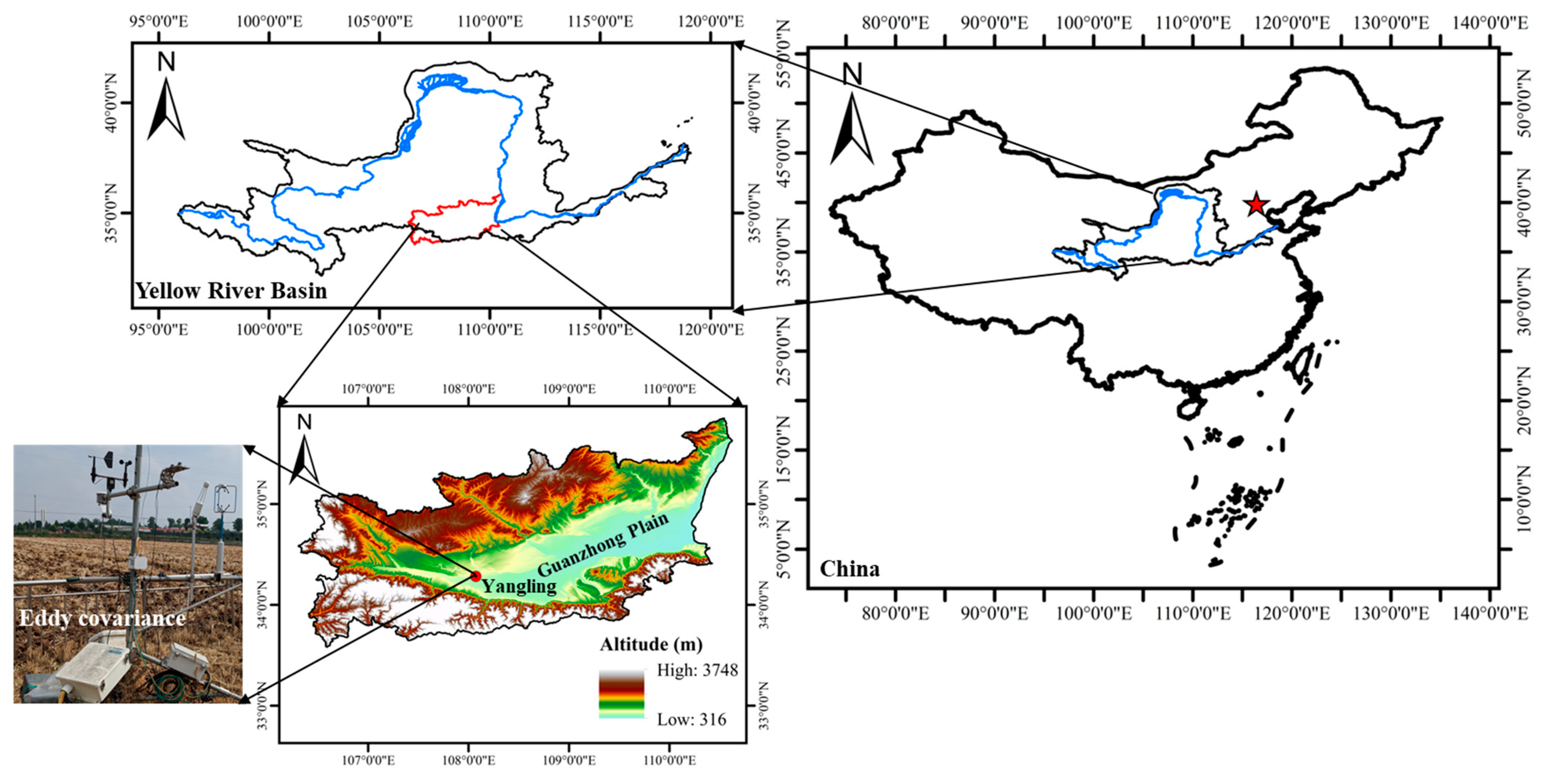
2.1. Study Site Description
2.2. Meteorological Data and Carbon Flux Measurements
2.3. Leaf Area Index Measurements
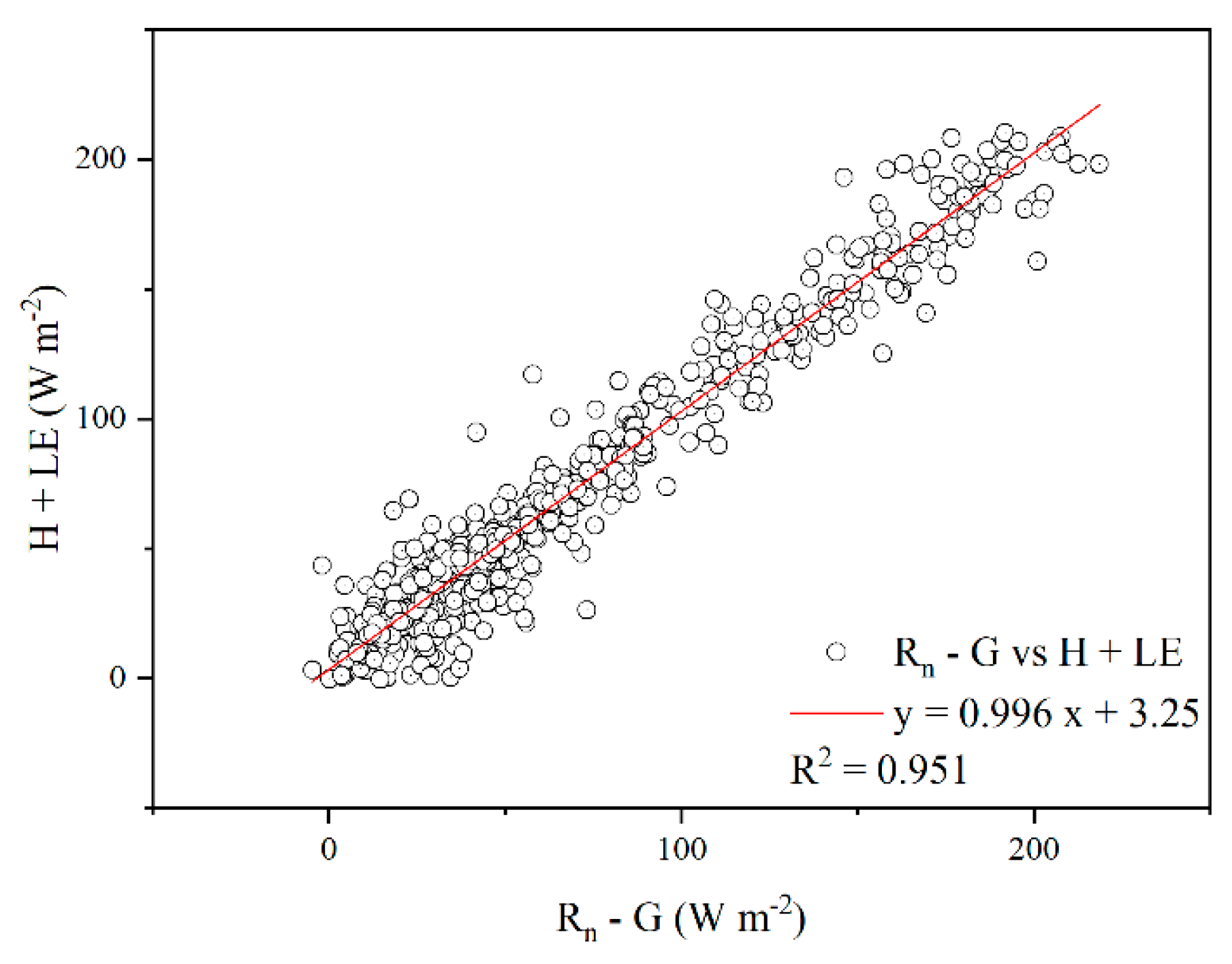
2.4. Flux Data Processing
2.5. Evapotranspiration Partitioning
2.6. Evapotranspiration Estimation
2.7. Statistical Analysis
3. Results
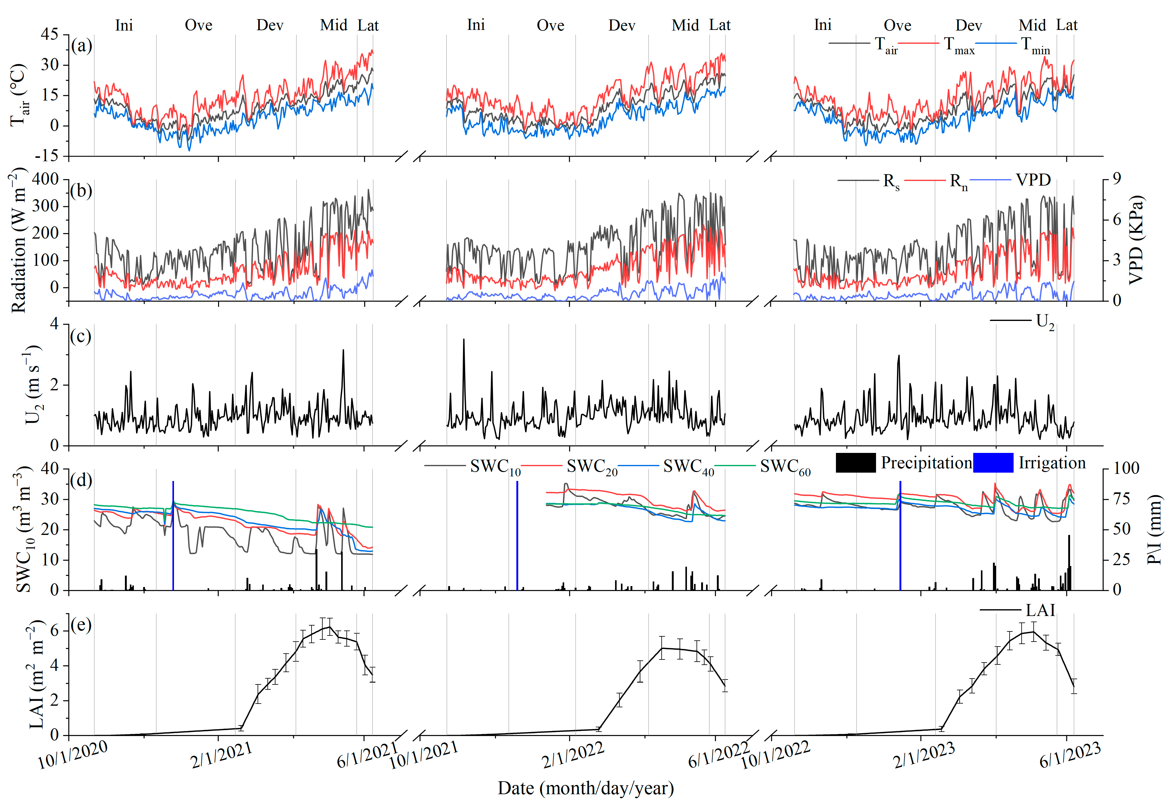
3.1. Variation in the Measured Environmental Variables
3.2. Seasonal Dynamics of the Evapotranspiration, Transpiration, and Soil Evaporation Rates
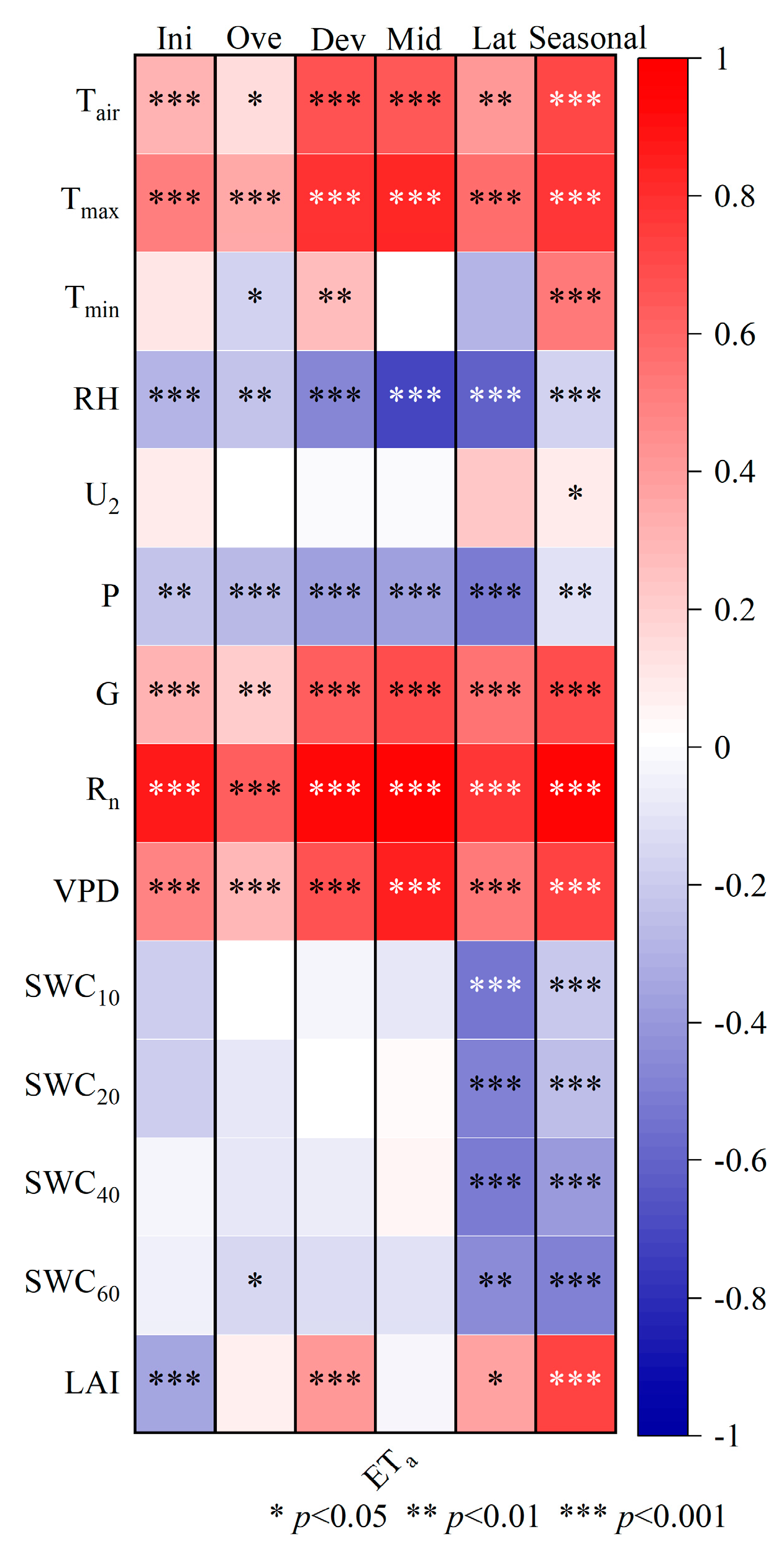
3.3. Relationships between the Measured Environmental Factors and Evapotranspiration Rates
3.4. Penman–Monteith-, Priestley–Taylor-, and Hargreaves-Equation-Based Crop Coefficients
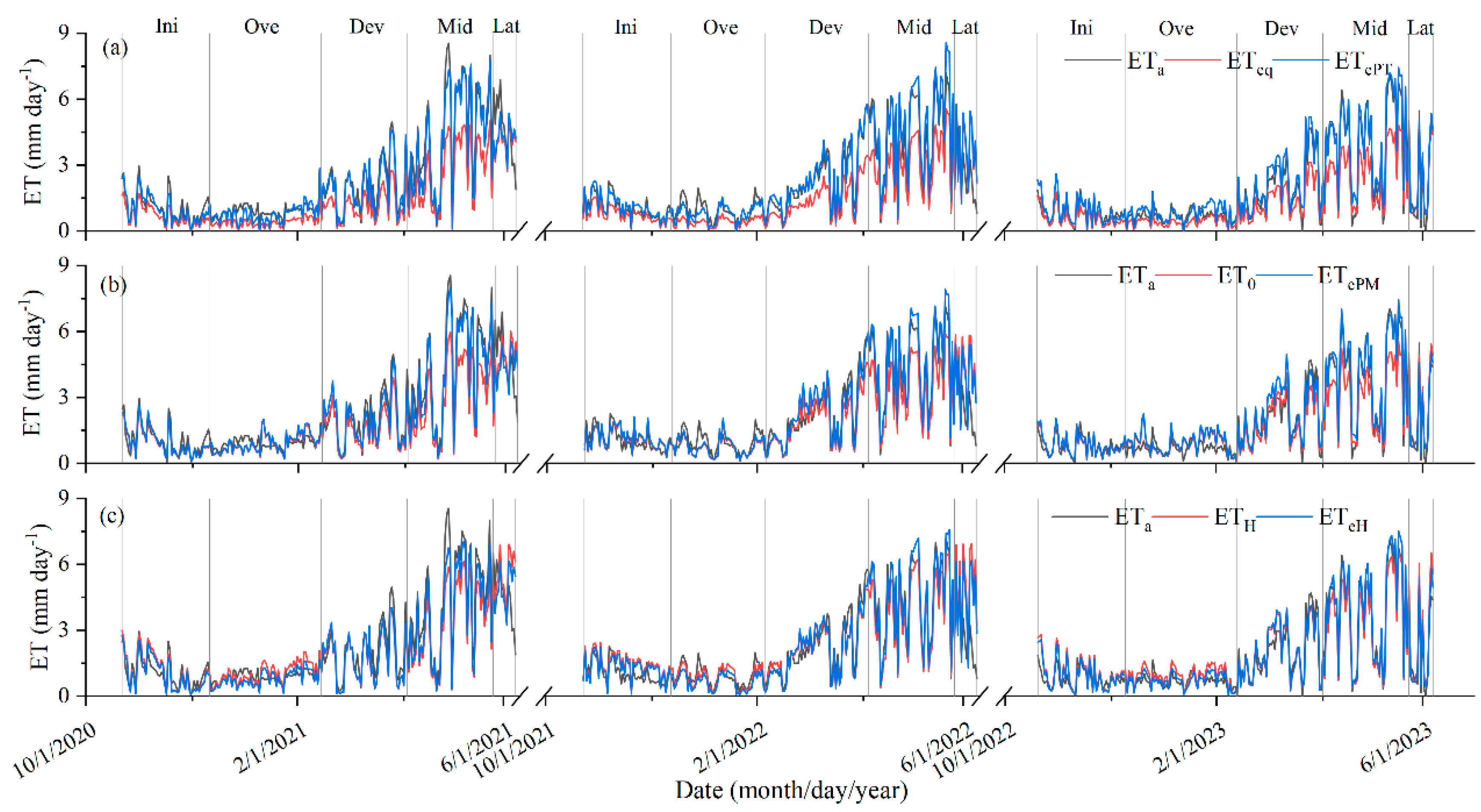
3.5. Evapotranspiration Estimation
4. Discussion
4.1. Controlling Factors of the Evapotranspiration Rate and T/ET Ratio
4.2. Evapotranspiration Partitioning of Winter Wheat Cropland in Other Regions Worldwide
4.3. Estimation Performances
5. Conclusions
- (1)
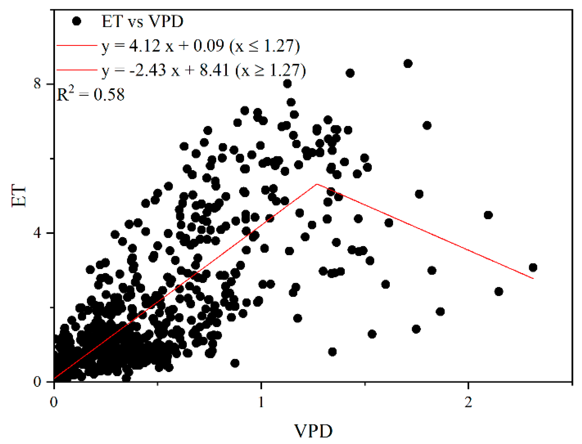
- T can be calculated by GPP∙/. The energy fluxes were the main limiting factor of in the three winter wheat growing seasons rather than water. In addition, the VPD values affected the change in the rates at a threshold of 1.27 KPa. The main limiting factors for T/ were VPD and LAI.
- (2)
- The cumulative rates of the 2020–2021, 2021–2022, and 2022–2023 winter wheat growing seasons were 501.3, 497.9, and 415.1 mm, respectively, in which E was the main contributor during the initial, overwintering, and late stages, while the T/ ratios during the middle stage exceeded 0.7. The average seasonal T/ and E/ ratios were 0.56 and 0.44, respectively.
- (3)
- The , α, and values showed a lack of obvious changes at the initial and overwintering stages of the cultivated winter wheat and tended to be concentrated from the developmental stage. The recommended values for winter wheat in the Guanzhong Plain at the Ini, Ove, Dev, Mid, and Lat stages were 1.05, 1.06, 1.21, 1.34, and 0.93, respectively; the recommended α values at the Ini, Ove, Dev, Mid, and Lat stages were 1.47, 1.95, 1.66, 1.54, and 1.04, respectively; the recommended values at the Ini, Ove, Dev, Mid, and Lat stages were 0.93, 0.99, 1.10, 1.21, and 0.80, respectively.
- (4)
- The models based on the adjusted , α, and models can reasonably estimate . However, the most accurate estimation was achieved using the PT-based crop coefficient.
- (5)
- Therefore, the PT-based method is expected to become a practical tool for formulating irrigation schedules for winter wheat cropland in the Guanzhong Plain and similar regions. We suggest further improvement of WUE in the future by reducing E rates through improved management measures (e.g., film mulch applications). The applicability of partitioning and model simulation to winter wheat cropland in other regions merits further study.
Author Contributions
Funding
Data Availability Statement
Acknowledgments
Conflicts of Interest
References
- Burba, G.; Verma, S.B. Seasonal and interannual variability in evapotranspiration of native tallgrass prairie and cultivated wheat ecosystems. Agric. For. Meteorol. 2005, 135, 190–201. [Google Scholar] [CrossRef]
- Kang, S.; Shi, W.; Zhang, J. An improved water-use efficiency for maize grown under regulated deficit irrigation. Field Crops Res. 2000, 67, 207–214. [Google Scholar] [CrossRef]
- Zhou, L.; Zhou, G. Measurement and modelling of evapotranspiration over a reed (Phragmites australis) marsh in Northeast China. J. Hydrol. 2009, 372, 41–47. [Google Scholar] [CrossRef]
- Rana, G.; Katerji, N. Measurement and estimation of actual evapotranspiration in the field under Mediterranean climate: A review. Eur. J. Agron. 2000, 13, 125–153. [Google Scholar] [CrossRef]
- Rafi, Z.; Merlin, O.; Le Dantec, V.; Khabba, S.; Mordelet, P.; Er-Raki, S.; Amazirh, A.; Olivera-Guerra, L.; Hssaine, B.A.; Simonneaux, V.; et al. Partitioning evapotranspiration of a drip-irrigated wheat crop: Inter-comparing eddy covariance-, sap flow-, lysimeter- and FAO-based methods. Agric. For. Meteorol. 2019, 265, 310–326. [Google Scholar] [CrossRef]
- Agam, N.; Evett, S.R.; Tolk, J.A.; Kustas, W.P.; Colaizzi, P.D.; Alfieri, J.G.; McKee, L.G.; Copeland, K.S.; Howell, T.A.; Chávez, J.L. Evaporative loss from irrigated interrows in a highly advective semi-arid agricultural area. Adv. Water Resour. 2012, 50, 20–30. [Google Scholar] [CrossRef]
- Eberbach, P.L.; Pala, M. Crop row spacing and its influence on the partitioning of evapotranspiration by winter-grown wheat in Northern Syria. Plant Soil 2004, 268, 195–208. [Google Scholar] [CrossRef]
- Hu, X.; Lei, H. Evapotranspiration partitioning and its interannual variability over a winter wheat-summer maize rotation system in the North China Plain. Agric. For. Meteorol. 2021, 310, 108635. [Google Scholar] [CrossRef]
- Kang, S.; Gu, B.; Du, T.; Zhang, J. Crop coefficient and ratio of transpiration to evapotranspiration of winter wheat and maize in a semi-humid region. Agric. Water Manag. 2003, 59, 239–254. [Google Scholar] [CrossRef]
- Ma, L.; Li, Y.; Wu, P.; Zhao, X.; Chen, X.; Gao, X. Coupling evapotranspiration partitioning with water migration to identify the water consumption characteristics of wheat and maize in an intercropping system. Agric. For. Meteorol. 2020, 290, 108034. [Google Scholar] [CrossRef]
- Ma, Y.; Song, X. Applying stable isotopes to determine seasonal variability in evapotranspiration partitioning of winter wheat for optimizing agricultural management practices. Sci. Total Environ. 2019, 654, 633–642. [Google Scholar] [CrossRef] [PubMed]
- Zhang, H.; Oweis, T.Y.; Garabet, S.; Pala, M. Water-use efficiency and transpiration efficiency of wheat under rain-fed conditions and supplemental irrigation in a Mediterranean-type environment. Plant Soil 1998, 201, 295–305. [Google Scholar] [CrossRef]
- Kool, D.; Agam, N.; Lazarovitch, N.; Heitman, J.L.; Sauer, T.J.; Ben-Gal, A. A review of approaches for evapotranspiration partitioning. Agric. For. Meteorol. 2014, 184, 56–70. [Google Scholar] [CrossRef]
- Allen, R.G.; Pereira, L.; Smith, M. Crop evapotranspiration-Guidelines for computing crop water requirements. Irrig. Drain. 1998, 56, 300. [Google Scholar]
- Sun, H.; Liu, C.; Zhang, X.; Shen, Y.; Zhang, Y. Effects of irrigation on water balance, yield and WUE of winter wheat in the North China Plain. Agric. Water Manag. 2006, 85, 211–218. [Google Scholar] [CrossRef]
- Boast, C.W.; Robertson, T.M. A “Micro-Lysimeter” Method for Determining Evaporation from Bare Soil: Description and Laboratory Evaluation. Soil Sci. Soc. Am. J. 1982, 46, 689–696. [Google Scholar] [CrossRef]
- Cammalleri, C.; Rallo, G.; Agnese, C.; Ciraolo, G.; Minacapilli, M.; Provenzano, G. Combined use of eddy covariance and sap flow techniques for partition of ET fluxes and water stress assessment in an irrigated olive orchard. Agric. Water Manag. 2013, 120, 89–97. [Google Scholar] [CrossRef]
- Jiang, X.; Kang, S.; Li, F.; Du, T.; Tong, L.; Comas, L.H. Evapotranspiration partitioning and variation of sap flow in female and male parents of maize for hybrid seed production in arid region. Agric. Water Manag. 2016, 176, 132–141. [Google Scholar] [CrossRef]
- Griffis, T.J. Tracing the flow of carbon dioxide and water vapor between the biosphere and atmosphere: A review of optical isotope techniques and their application. Agric. For. Meteorol. 2013, 174, 85–109. [Google Scholar] [CrossRef]
- Nelson, J.A.; Pérez-Priego, O.; Zhou, S.; Poyatos, R.; Zhang, Y.; Blanken, P.D.; Gimeno, T.E.; Wohlfahrt, G.; Desai, A.R.; Gioli, B.; et al. Ecosystem transpiration and evaporation: Insights from three water flux partitioning methods across FLUXNET sites. Glob. Change Biol. 2020, 26, 6916–6930. [Google Scholar] [CrossRef]
- Cowan, I.R.L.; Farquhar, G.D. Stomatal function in relation to leaf metabolism and environment. Symp. Soc. Exp. Biol. 1977, 31, 471–505. [Google Scholar] [PubMed]
- Zhou, S.; Yu, B.; Huang, Y.; Wang, G. The effect of vapor pressure deficit on water use efficiency at the subdaily time scale. Geophys. Res. Lett. 2014, 41, 5005–5013. [Google Scholar] [CrossRef]
- Zhou, S.; Yu, B.; Huang, Y.; Wang, G. Daily underlying water use efficiency for AmeriFlux sites. J. Geophys. Res. Biogeosci. 2015, 120, 887–902. [Google Scholar] [CrossRef]
- Liu, C.; Zhang, X.; Zhang, Y. Determination of daily evaporation and evapotranspiration of winter wheat and maize by large-scale weighing lysimeter and micro-lysimeter. Agric. For. Meteorol. 2002, 111, 109–120. [Google Scholar] [CrossRef]
- Qiu, R.; Liu, C.; Cui, N.; Wu, Y.; Wang, Z.; Li, G. Evapotranspiration estimation using a modified Priestley-Taylor model in a rice-wheat rotation system. Agric. Water Manag. 2019, 224, 105755. [Google Scholar] [CrossRef]
- Zhang, B.; Liu, Y.; Xu, D.; Zhao, N.; Lei, B.; Rosa, R.D.; Paredes, P.; Paço, T.A.; Pereira, L.S. The dual crop coefficient approach to estimate and partitioning evapotranspiration of the winter wheat-summer maize crop sequence in North China Plain. Irrig. Sci. 2013, 31, 1303–1316. [Google Scholar] [CrossRef]
- Baldocchi, D.D. Assessing the eddy covariance technique for evaluating carbon dioxide exchange rates of ecosystems: Past, present and future. Glob. Change Biol. 2003, 9, 479–492. [Google Scholar] [CrossRef]
- Alberto, M.C.R.; Quilty, J.R.; Buresh, R.J.; Wassmann, R.; Haidar, S.; Correa, T.Q., Jr.; Sandro, J.M. Actual evapotranspiration and dual crop coefficients for dry-seeded rice and hybrid maize grown with overhead sprinkler irrigation. Agric. Water Manag. 2014, 136, 1–12. [Google Scholar] [CrossRef]
- Wang, Y.; Zou, Y.; Cai, H.; Zeng, Y.; He, J.; Yu, L.; Zhang, C.; Saddique, Q.; Peng, X.; Siddique, K.H.; et al. Seasonal variation and controlling factors of evapotranspiration over dry semi-humid cropland in Guanzhong Plain, China. Agric. Water Manag. 2022, 259, 107242. [Google Scholar] [CrossRef]
- Nikolaou, G.; Neocleous, D.; Kitta, E.; Katsoulas, N. Assessment of the Priestley-Taylor coefficient and a modified potential evapotranspiration model. Smart Agric. Technol. 2022, 3, 100075. [Google Scholar] [CrossRef]
- Qiu, R.; Li, L.; Liu, C.; Wang, Z.; Zhang, B.; Liu, Z. Evapotranspiration estimation using a modified crop coefficient model in a rotated rice-winter wheat system. Agric. Water Manag. 2022, 264, 107501. [Google Scholar] [CrossRef]
- Xiang, K.; Li, Y.; Horton, R.; Feng, H. Similarity and difference of potential evapotranspiration and reference crop evapotranspiration—A review. Agric. Water Manag. 2020, 232, 106043. [Google Scholar] [CrossRef]
- Hargreaves, G.H. Moisture availability and crop production. Trans. ASAE 1975, 18, 980–984. [Google Scholar] [CrossRef]
- Priestley, C.H.B.; Taylor, R. On the assessment of surface heat flux and evaporation using large-scale parameters. Mon. Weather Rev. 1972, 100, 81–92. [Google Scholar] [CrossRef]
- Zhao, H.; Shar, A.G.; Li, S.; Chen, Y.; Shi, J.; Zhang, X.; Tian, X. Effect of straw return mode on soil aggregation and aggregate carbon content in an annual maize-wheat double cropping system. Soil Tillage Res. 2018, 175, 178–186. [Google Scholar] [CrossRef]
- Zhang, Y.; Li, C.; Wang, Y.; Hu, Y.; Christie, P.; Zhang, J.; Li, X. Maize yield and soil fertility with combined use of compost and inorganic fertilizers on a calcareous soil on the North China Plain. Soil Tillage Res. 2016, 155, 85–94. [Google Scholar] [CrossRef]
- Wang, Y.; Cai, H.; Yu, L.; Peng, X.; Xu, J.; Wang, X. Evapotranspiration partitioning and crop coefficient of maize in dry semi-humid climate regime. Agric. Water Manag. 2020, 236, 106164. [Google Scholar] [CrossRef]
- Zheng, J.; Fan, J.; Zhang, F.; Zhuang, Q. Evapotranspiration partitioning and water productivity of rainfed maize under contrasting mulching conditions in Northwest China. Agric. Water Manag. 2021, 243, 106473. [Google Scholar] [CrossRef]
- Yu, L.; Zeng, Y.; Su, Z.; Cai, H.; Zheng, Z. The effect of different evapotranspiration methods on portraying soil water dynamics and ET partitioning in a semi-arid environment in Northwest China. Hydrol. Earth Syst. Sci. 2016, 20, 975–990. [Google Scholar] [CrossRef]
- Campbell, G.S.; Norman, J.M. (Eds.) An Introduction to Environmental Biophysics; Springer Science & Business Media: Berlin/Heidelberg, Germany, 1977. [Google Scholar]
- Wang, Y.; Hu, C.; Dong, W.; Li, X.; Zhang, Y.; Qin, S.; Oenema, O. Carbon budget of a winter-wheat and summer-maize rotation cropland in the North China Plain. Agric. Ecosyst. Environ. 2015, 206, 33–45. [Google Scholar] [CrossRef]
- Mckee, G.W. A Coefficient for Computing Leaf Area in Hybrid Corn. Agron. J. 1964, 56, 240–241. [Google Scholar] [CrossRef]
- Vickers, D.; Mahrt, L. Quality Control and Flux Sampling Problems for Tower and Aircraft Data. J. Atmos. Ocean. Technol. 1997, 14, 512–526. [Google Scholar] [CrossRef]
- Tanner, C.B.; Thurtell, G.W. (Eds.) Anemoclinometer Measurements of Reynolds Stress and Heat Transport in the Atmospheric Surface Layer; The Laboratory: Blackwood, NJ, USA, 1969. [Google Scholar]
- Moncrieff, J.B.; Clement, R.J.; Finnigan, J.; Meyers, T.P. (Eds.) Averaging, Detrending, and Filtering of Eddy Covariance Time Series; Springer Netherlands: Dordrecht, The Netherlands, 2004. [Google Scholar]
- Webb, E.K.; Pearman, G.I.; Leuning, R. Correction of flux measurements for density effects due to heat and water vapour transfer. Q. J. R. Meteorol. Soc. 1980, 106, 85–100. [Google Scholar] [CrossRef]
- Gash, J.H.C.; Culf, A.D. Applying a linear detrend to eddy correlation data in realtime. Bound. Layer Meteorol. 1996, 79, 301–306. [Google Scholar] [CrossRef]
- Zhu, Z.; Sun, X.-M.; Wen, X.; Zhou, Y.; Tian, J.; Yuan, G. Study on the processing method of nighttime CO2 eddy covariance flux data in ChinaFLUX. Sci. China Ser. D Earth Sci. 2006, 49, 36–46. [Google Scholar] [CrossRef]
- Wutzler, T.; Lucas-Moffat, A.; Migliavacca, M.; Knauer, J.; Sickel, K.; Šigut, L.; Menzer, O.; Reichstein, M. Basic and extensible post-processing of eddy covariance flux data with REddyProc. Biogeosciences 2018, 15, 5015–5030. [Google Scholar] [CrossRef]
- Twine, T.E.; Kustas, W.P.; Norman, J.M.; Cook, D.R.; Houser, P.; Meyers, T.P.; Prueger, J.H.; Starks, P.J.; Wesely, M.L. Correcting eddy-covariance flux underestimates over a grassland. Agric. For. Meteorol. 2000, 103, 279–300. [Google Scholar] [CrossRef]
- Reichstein, M.; Falge, E.; Baldocchi, D.; Papale, D.; Aubinet, M.; Berbigier, P.; Bernhofer, C.; Buchmann, N.; Gilmanov, T.; Granier, A.; et al. On the separation of net ecosystem exchange into assimilation and ecosystem respiration: Review and improved algorithm. Glob. Change Biol. 2005, 11, 1424–1439. [Google Scholar] [CrossRef]
- Lloyd, J.; Taylor, J.A. On the temperature-dependence of soil respiration. Funct. Ecol. 1994, 8, 315–323. [Google Scholar] [CrossRef]
- Aubinet, M.; Chermanne, B.; Vandenhaute, M.; Longdoz, B.; Yernaux, M.; Laitat, E. Long term carbon dioxide exchange above a mixed forest in the Belgian Ardennes. Agric. For. Meteorol. 2001, 108, 293–315. [Google Scholar] [CrossRef]
- Zhou, S.; Yu, B.; Zhang, Y.; Huang, Y.; Wang, G. Partitioning evapotranspiration based on the concept of underlying water use efficiency. Water Resour. Res. 2016, 52, 1160–1175. [Google Scholar] [CrossRef]
- Mcnaughton, K.G.; Spriggs, T.W. A mixed-layer model for regional evaporation. Bound. Layer Meteorol. 1986, 34, 243–262. [Google Scholar] [CrossRef]
- Lei, H.; Yang, D. Interannual and seasonal variability in evapotranspiration and energy partitioning over an irrigated cropland in the North China Plain. Agric. For. Meteorol. 2010, 150, 581–589. [Google Scholar] [CrossRef]
- Ding, R.; Kang, S.; Li, F.; Zhang, Y.; Tong, L. Evapotranspiration measurement and estimation using modified Priestley–Taylor model in an irrigated maize field with mulching. Agric. For. Meteorol. 2013, 168, 140–148. [Google Scholar] [CrossRef]
- Shen, Y.; Zhang, Y.; Scanlon, B.R.; Lei, H.; Yang, D.; Yang, F. Energy/water budgets and productivity of the typical croplands irrigated with groundwater and surface water in the North China Plain. Agric. For. Meteorol. 2013, 181, 133–142. [Google Scholar] [CrossRef]
- Marques, T.V.; Mendes, K.; Mutti, P.; Medeiros, S.; Silva, L.; Perez-Marin, A.M.; Campos, S.; Lúcio, P.S.; Lima, K.; dos Reis, J.; et al. Environmental and biophysical controls of evapotranspiration from Seasonally Dry Tropical Forests (Caatinga) in the Brazilian Semiarid. Agric. For. Meteorol. 2020, 287, 107957. [Google Scholar] [CrossRef]
- Chen, S.; Wei, W.; Tong, B.; Chen, L. Effects of soil moisture and vapor pressure deficit on canopy transpiration for two coniferous forests in the Loess Plateau of China. Agric. For. Meteorol. 2023, 339, 109581. [Google Scholar] [CrossRef]
- Pérez-Priego, Ó.; Testi, L.; Orgaz, F.; Villalobos, F.J. A large closed canopy chamber for measuring CO2 and water vapour exchange of whole trees. Environ. Exp. Bot. 2010, 68, 131–138. [Google Scholar] [CrossRef]
- Wei, Z.; Yoshimura, K.; Wang, L.; Miralles, D.G.; Jasechko, S.; Lee, X. Revisiting the contribution of transpiration to global terrestrial evapotranspiration. Geophys. Res. Lett. 2017, 44, 2792–2801. [Google Scholar] [CrossRef]
- Berkelhammer, M.; Noone, D.C.; Wong, T.E.; Burns, S.P.; Knowles, J.F.; Kaushik, A.; Blanken, P.D.; Williams, M.W. Convergent approaches to determine an ecosystem’s transpiration fraction. Glob. Biogeochem. Cycles 2016, 30, 933–951. [Google Scholar] [CrossRef]
- Balwinder-Singh Eberbach, P.L.; Humphreys, E.; Kukal, S.S. The effect of rice straw mulch on evapotranspiration, transpiration and soil evaporation of irrigated wheat in Punjab, India. Agric. Water Manag. 2011, 98, 1847–1855. [Google Scholar] [CrossRef]
- Yu, L.P.; Huang, G.H.; Liu, H.J.; Wang, X.P.; Wang, M.Q. Experimental Investigation of Soil Evaporation and Evapotranspiration of Winter Wheat Under Sprinkler Irrigation. Agric. Sci. China 2009, 8, 1360–1368. [Google Scholar] [CrossRef]
- Liao, Y.; Cao, H.X.; Liu, X.; Li, H.T.; Hu, Q.Y.; Xue, W.K. By increasing infiltration and reducing evaporation, mulching can improve the soil water environment and apple yield of orchards in semiarid areas. Agric. Water Manag. 2021, 253, 106936. [Google Scholar] [CrossRef]
- Sumner, D.M.; Jacobs, J.M. Utility of Penman–Monteith, Priestley–Taylor, reference evapotranspiration, and pan evaporation methods to estimate pasture evapotranspiration. J. Hydrol. 2005, 308, 81–104. [Google Scholar] [CrossRef]
- Gong, X.; Qiu, R.; Ge, J.; Bo, G.; Ping, Y.; Xin, Q.; Wang, S. Evapotranspiration partitioning of greenhouse grown tomato using a modified Priestley–Taylor model. Agric. Water Manag. 2021, 247, 106709. [Google Scholar] [CrossRef]
- Ershadi, A.; Mccabe, M.F.; Evans, J.P.; Chaney, N.W.; Wood, E.F. Multi-site evaluation of terrestrial evaporation models using FLUXNET data. Agric. For. Meteorol. 2014, 187, 46–61. [Google Scholar] [CrossRef]
- Feng, Y.; Yue, J.; Cui, N.; Zhao, L.; Chen, L.; Gong, D. Calibration of Hargreaves model for reference evapotranspiration estimation in Sichuan basin of southwest China. Agric. Water Manag. 2017, 181, 1–9. [Google Scholar] [CrossRef]


| Growth Stage | Period (Month/Day/Year) | Days after Sowing | Rn (MJ m−2) | LE (MJ m−2) | Tair (°C) | VPD (kPa) | P + I (mm) | SWC (m3 m−3) | LAImax (m2 m−2) | |
|---|---|---|---|---|---|---|---|---|---|---|
| 2020–2021 Winter wheat | Ini | 22 October 2020–11 December 2020 | 0–50 | 127.9 | 125.3 | 7.3 | 0.32 | 44 + 0 | 25.5 | 0.11 |
| Ove | 12 December 2020–14 February 2021 | 51–115 | 114.0 | 124.6 | 1.7 | 0.40 | 2 + 90 | 24.5 | 0.38 | |
| Dev | 15 February 2021–5 April 2021 | 116–165 | 265.7 | 253.7 | 9.5 | 0.46 | 39 + 0 | 20.9 | 4.7 | |
| Mid | 6 April 2021–25 May 2021 | 166–215 | 521.4 | 534.5 | 16.4 | 0.64 | 97 + 0 | 20.1 | 6.23 | |
| Lat | 26 May 2021–8 June 2021 | 216–229 | 202.0 | 159.5 | 23.9 | 1.87 | 3 + 0 | 15.6 | 5.38 | |
| Seasonal | 22 October 2020–8 June 2021 | 0–229 | 1231.0 | 1197.6 | 9.2 | 0.52 | 185 + 90 | 22.4 | 6.23 | |
| 2021–2022 Winter wheat | Ini | 0–50 | 153.2 | 106.3 | 7.1 | 0.39 | 11 + 0 | 0.10 | ||
| Ove | 23 October 2021–12 December 2021 | 51–115 | 137.9 | 99.5 | 1.2 | 0.24 | 23 + 90 | 0.32 | ||
| Dev | 13 December 2021–15 February 2022 | 116–165 | 338.9 | 290.9 | 9.9 | 0.59 | 31 + 0 | 29.3 | 4.1 | |
| Mid | 16 February 2022–6 April 2022 | 166–215 | 588.0 | 521.6 | 17.1 | 0.78 | 97 + 0 | 26.1 | 5.01 | |
| Lat | 7 April 2022–26 May 2022 | 216–229 | 170.4 | 84.6 | 23.6 | 1.56 | 13 + 0 | 24.7 | 4.17 | |
| Seasonal | 27 May 2022–9 June 2022 | 0–229 | 1388.3 | 1102.9 | 9.2 | 0.53 | 174 + 90 | 5.01 | ||
| 2022–2023 Winter wheat | Ini | 23 October 2021–9 June 2022 | 0–50 | 108.7 | 98.7 | 8.1 | 0.24 | 17 + 0 | 29.2 | 0.07 |
| Ove | 51–115 | 121.9 | 104.2 | 1.0 | 0.36 | 7 + 90 | 28.9 | 0.35 | ||
| Dev | 20 October 2022–9 December 2022 | 116–165 | 306.7 | 243.3 | 9.1 | 0.54 | 81 + 0 | 28.2 | 4.4 | |
| Mid | 10 December 2022–12 February 2023 | 166–215 | 531.0 | 523.4 | 16.2 | 0.72 | 74 + 0 | 27.2 | 5.94 | |
| Lat | 13 February 2023–3 April 2023 | 216–230 | 125.5 | 74.6 | 18.7 | 0.48 | 121 + 0 | 28.2 | 4.97 | |
| Seasonal | 4 April 2023–23 May 2023 | 0–230 | 1193.7 | 1044.3 | 8.7 | 0.45 | 300 + 90 | 28.3 | 5.94 |
| Winter Wheat Growing Season | Slope | Intercept | |
|---|---|---|---|
| 22 October 2020–8 June 2021 | 1.02 | 5.08 | 0.97 |
| 23 October 2021–9 June 2022 | 0.98 | 0.01 | 0.96 |
| 20 October 2022–7 June 2023 | 1.00 | 4.01 | 0.93 |
| Average | 0.996 | 3.25 | 0.95 |
| Growth Stage | (mm) | T (mm) | E (mm) | |||
|---|---|---|---|---|---|---|
| 2020–2021 winter wheat growing season | Ini | 55.2 | 8.4 | 46.8 | 0.15 | 0.85 |
| Ove | 58.5 | 23.1 | 35.4 | 0.39 | 0.61 | |
| Dev | 103.1 | 75.1 | 28.0 | 0.73 | 0.27 | |
| Mid | 219.6 | 156.8 | 62.8 | 0.71 | 0.29 | |
| Lat | 64.9 | 15.6 | 49.3 | 0.24 | 0.76 | |
| Seasonal | 501.3 | 279.0 | 222.3 | 0.56 | 0.44 | |
| 2021–2022 winter wheat growing season | Ini | 54.1 | 10.1 | 44.0 | 0.19 | 0.81 |
| Ove | 61.5 | 11.4 | 50.1 | 0.19 | 0.81 | |
| Dev | 122.9 | 89.0 | 33.9 | 0.72 | 0.28 | |
| Mid | 222.1 | 165.7 | 56.5 | 0.75 | 0.25 | |
| Lat | 37.3 | 7.6 | 29.7 | 0.20 | 0.80 | |
| Seasonal | 497.9 | 283.8 | 214.1 | 0.57 | 0.43 | |
| 2022–2023 winter wheat growing season | Ini | 40.8 | 4.8 | 36.0 | 0.12 | 0.88 |
| Ove | 45.0 | 15.2 | 29.8 | 0.34 | 0.66 | |
| Dev | 99.4 | 65.2 | 34.2 | 0.66 | 0.34 | |
| Mid | 194.7 | 138.0 | 56.7 | 0.71 | 0.29 | |
| Lat | 35.2 | 9.5 | 25.7 | 0.27 | 0.73 | |
| Seasonal | 415.1 | 232.7 | 182.4 | 0.56 | 0.44 | |
| Three-year average | Ini | 50.0 | 7.8 | 42.3 | 0.16 | 0.84 |
| Ove | 55.0 | 16.6 | 38.4 | 0.30 | 0.70 | |
| Dev | 108.5 | 76.4 | 32.0 | 0.70 | 0.30 | |
| Mid | 212.1 | 153.5 | 58.7 | 0.72 | 0.28 | |
| Lat | 45.8 | 10.9 | 34.9 | 0.24 | 0.76 | |
| Seasonal | 471.4 | 265.2 | 206.3 | 0.56 | 0.44 |
| Growth Stage | α | |||
|---|---|---|---|---|
| 2020–2021 winter wheat growing season | Ini | 1.16 | 1.62 | 1.09 |
| Ove | 1.11 | 2.10 | 0.99 | |
| Dev | 1.30 | 1.76 | 1.18 | |
| Mid | 1.46 | 1.64 | 1.30 | |
| Lat | 0.99 | 1.15 | 0.87 | |
| Seasonal | 1.20 | 1.65 | 1.09 | |
| 2021–2022 winter wheat growing season | Ini | 0.96 | 1.42 | 0.77 |
| Ove | 1.23 | 2.04 | 1.18 | |
| Dev | 1.21 | 1.70 | 1.10 | |
| Mid | 1.27 | 1.47 | 1.18 | |
| Lat | 0.68 | 0.82 | 0.65 | |
| Seasonal | 1.07 | 1.49 | 0.98 | |
| 2022–2023 winter wheat growing season | Ini | 1.03 | 1.37 | 0.92 |
| Ove | 0.86 | 1.71 | 0.79 | |
| Dev | 1.11 | 1.53 | 1.03 | |
| Mid | 1.29 | 1.51 | 1.15 | |
| Lat | 1.11 | 1.15 | 0.89 | |
| Seasonal | 1.08 | 1.45 | 0.96 | |
| Average | Ini | 1.05 | 1.47 | 0.93 |
| Ove | 1.06 | 1.95 | 0.99 | |
| Dev | 1.21 | 1.66 | 1.10 | |
| Mid | 1.34 | 1.54 | 1.21 | |
| Lat | 0.93 | 1.04 | 0.80 | |
| Seasonal | 1.12 | 1.53 | 1.01 |
| 2020–2021 winter wheat | 501.3 | 312.5 | 467.7 | 407.6 | 477.9 | 456.4 | 456.8 |
| 2020–2021 winter wheat | 497.9 | 345.8 | 526.4 | 444.0 | 527.8 | 507.4 | 514.6 |
| 2020–2021 winter wheat | 415.1 | 296.7 | 457.1 | 384.4 | 460.0 | 428.6 | 436.3 |
| Seasonal average values | 471.4 | 318.3 | 483.7 | 412.0 | 488.6 | 464.1 | 469.2 |
| Sites | Measurement Methods | Periods | (mm) | T (mm) | E (mm) | References | ||
|---|---|---|---|---|---|---|---|---|
| Yangling, Shaanxi, China (34°17′45″ N, 108°04′07″ E) | EC | 2020–2021 | 501.3 | 279.0 | 222.3 | 0.56 | 0.44 | This study |
| 2021–2022 | 497.9 | 283.8 | 214.1 | 0.57 | 0.43 | |||
| 2022–2023 | 415.1 | 232.7 | 182.4 | 0.56 | 0.44 | |||
| Weishan, Shandong, China (36°38′55″ N, 116°03′15″ E) | EC | 2005–2019 | 21 | 22 | 13 | 0.65–0.82 | 0.18–0.35 | [8] |
| Yangling, Shaanxi, China (34°20′ N, 108°04′ E) | Water balance method | 2014–2015 | 413.8 | 304.1 | 93.7 | 0.73 | 0.27 | [10] |
| 2015–2016 | 373.6 | 262.3 | 98.0 | 0.70 | 0.30 | |||
| Daxing, Beijing, China (39°37′ N, 116°26′ E) | Soil water balance | 2013–2014 | 27.7 | 24.5 | 4.5 | 0.01 | [11] | |
| 2014–2015 | 39.9 | 34.5 | 15.1 | 0.04 | ||||
| Nanjing, Jiangsu, China (32.21 ° N, 118.68 ° E) | Bowen ratio energy balance | 2016–2017 | 285.4 | 149.6 | 135.8 | 0.52 | 0.48 | [25] |
| 2017–2018 | 279.4 | 137.0 | 142.4 | 0.49 | 0.51 | |||
| Daxing, Beijing, China (39°37′ N, 116°26′ E) | Eddy covariance | 2007–2008 | 396.3 | 287.0 | 109.3 | 0.72 | 0.28 | [26] |
| 2008–2009 | 437.3 | 287.0 | 122.1 | 0.72 | 0.28 | |||
| Ludhiana, Punjab, India (30°56′ N, 75°52′ E) | Water balance method | 2006–2007 | 340–345 | 210–240 | 100–135 | 0.61–0.70 | 0.30–0.39 | [64] |
| 2007–2008 | 400–404 | 243–279 | 121–161 | 0.60–0.70 | 0.30–0.40 | |||
| Tongzhou, Beijing, China (39°36′ N; 116°48′ E) | Water balance method | 2006–2007 | 219–486 | 65.7–77.9 | 0.72–0.79 | 0.21–0.28 | [65] | |
| Luancheng, China (37°50′ N,114°40′ E) | Soil water balance | 1999–2000 | 192.0–464.0 | 84.0–323.6 | 108.0–140.4 | 0.46–0.70 | 0.30–0.56 | [15] |
| 2000–2001 | 241.3–443.7 | 132.6–300.7 | 108.7–143.0 | 0.56–0.68 | 0.32–0.45 | |||
| 2001–2002 | 259.7–444.9 | 161.9–326.2 | 97.9–139.9 | 0.64–0.76 | 0.24–0.37 | |||
|
Yangling, Shaanxi, China (34°20′ N, 108°24′ E) | Lysimeter | 1987–1997 | 43.9 | 46.9 | 21.8 | 0.67 | 0.33 | [9] |
|
Tel Hadya, Syria (35°55′ N 37°10′ E) | Water balance method | 1996–1997 | 367.3–376.7 | 172.1–184.8 | 182.5–204.6 | 0.50–0.55 | 0.50–0.55 | [7] |
| Luancheng, China (37°50′ N, 114°40′ E) | Lysimeter | 1995–2000 | 401.2–479.2 | 0.70 | 0.30 | [24] | ||
| Tel Hadya, Syria (36°01′ N, 36°56′ E) | Water balance method | 1991–1996 | 295–456 | 131–358 | 91–179 | 0.44–0.80 | 0.20–0.56 | [12] |
Disclaimer/Publisher’s Note: The statements, opinions and data contained in all publications are solely those of the individual author(s) and contributor(s) and not of MDPI and/or the editor(s). MDPI and/or the editor(s) disclaim responsibility for any injury to people or property resulting from any ideas, methods, instructions or products referred to in the content. |
© 2023 by the authors. Licensee MDPI, Basel, Switzerland. This article is an open access article distributed under the terms and conditions of the Creative Commons Attribution (CC BY) license (https://creativecommons.org/licenses/by/4.0/).
Share and Cite
Peng, X.; Liu, X.; Wang, Y.; Cai, H. Evapotranspiration Partitioning and Estimation Based on Crop Coefficients of Winter Wheat Cropland in the Guanzhong Plain, China. Agronomy 2023, 13, 2982. https://doi.org/10.3390/agronomy13122982
Peng X, Liu X, Wang Y, Cai H. Evapotranspiration Partitioning and Estimation Based on Crop Coefficients of Winter Wheat Cropland in the Guanzhong Plain, China. Agronomy. 2023; 13(12):2982. https://doi.org/10.3390/agronomy13122982
Chicago/Turabian StylePeng, Xiongbiao, Xuanang Liu, Yunfei Wang, and Huanjie Cai. 2023. "Evapotranspiration Partitioning and Estimation Based on Crop Coefficients of Winter Wheat Cropland in the Guanzhong Plain, China" Agronomy 13, no. 12: 2982. https://doi.org/10.3390/agronomy13122982
APA StylePeng, X., Liu, X., Wang, Y., & Cai, H. (2023). Evapotranspiration Partitioning and Estimation Based on Crop Coefficients of Winter Wheat Cropland in the Guanzhong Plain, China. Agronomy, 13(12), 2982. https://doi.org/10.3390/agronomy13122982