1. Introduction
Yield mapping is an essential component of precision agriculture [
1]. Combine harvesters equipped with yield monitors consisting of yield sensors and global navigation satellite systems (GNSS) were crucial elements in the development of precision agriculture because they were one of the first means to characterize the within-field variability in crop yield [
1,
2,
3]. Yield monitors have been available on the market since the early 1990s, and there is comprehensive research on yield monitoring and yield variability within fields [
4,
5].
The global level of adoption of yield monitoring and yield maps is relatively unknown. Most existing studies focus on North America, which has the greatest adoption level [
6,
7]. Schimmelpfennig [
7] reported that yield monitors were used on roughly 70% of the United States corn and soybean acres in 2010–2012. European studies indicate lower levels of adoption [
8], and there is evidence that most yield monitors are used to visualize the real-time yield during harvest and not as data providers for yield maps [
7,
8]. Lachia et al. [
8] reported that the use of yield maps is too complex for the majority of farmers.
Despite the apparent challenges of using yield monitors to produce yield maps as a basis for decision-making, the scientific community’s interest in yield monitoring has decreased during the last decades [
9]. Research seems to have lost its attractiveness in favor of newer topics such as remote sensing [
10] and the use of unmanned aerial vehicles (UAVs) [
11].
Crop yield predictions are based on either data-driven or process-based models. In data-driven models, empirical models are based on observed data, such as vegetation indices (VI) derived from spectral sensing and corresponding crop yields [
12]. Such models are considered black-box models since they do not explain the mechanism that drives the yield. Nevertheless, they are evaluated to be the most practical models for yield predictions with few inputs [
13] and are useful for precision agricultural contexts. Detailed information on crop growth and phenology is required to achieve information about the mechanisms behind the yield. Process-based models are helpful in regional yield forecasting systems [
14] but far too data demanding in precision agricultural contexts.
Regarding grass seed production, knowledge about yield variability within fields is particularly sparse. To the authors’ knowledge, only one study in perennial ryegrass (
Lolium perenne L.) has been published, concluding that the yield estimates of yield monitors on combine harvesters vary substantially from previous or subsequent observations, even over an apparently uniform ryegrass field [
15]. The main reasons are that the amount of seed biomass or seed volume is significantly less than for cereals, maize, and soybean and that the biomass of stems, leaves and chaff (material other than grain) is relatively greater. Therefore, it is not possible to achieve reliable yield maps based on data from yield monitors mounted on combine harvesters.
The increasing use of UAVs opens new possibilities for remote sensing of crops and providing yield estimates [
16]. A simple approach in yield estimation based on UAV imagery is to establish relationships between VI and crop yield [
17]. VI are computed using several spectral bands sensitive to plant biomass and vigor, and there are two major groups of VI. One group includes spectral bands in the invisible spectrum, and another includes spectral bands exclusively in the visible spectrum. The first group requires multispectral cameras for image acquisition, and the second group can be acquired with RGB cameras. Both types of VI may be suitable for yield estimations [
18] because they reflect the vigor, LAI, and other physical characteristics of the crop [
19].
Suppose it is possible to establish linear or non-linear relationships between VI and crop yield, then regression models can be used to predict yield. In a previous study, Jensen et al. [
20] investigated different selection strategies for training regression models to predict the density of annual grass weeds in cereals based on VI derived from UAV color images. The study showed that training based on selection from extreme values in the field provided better prediction accuracy than random selection. Furthermore, the study showed that simple linear prediction models offered a valuable alternative to a more complex random forest machine-learning algorithm [
20].
The color, and thereby the spectral signature, of red fescue crops depends on several factors such as the degree of lodging, the variety, the fertilizer, soil conditions, and drought [
21]. The seed yield is also affected by the time that lodging and fertilization take place [
21]. Therefore, it is extremely difficult to develop generalized models describing the relation between spectral characteristics and the yield variation in a specific field. In general, research in yield predictive models should focus on generalized models to be applied elsewhere and across various temporal scales. However, this study motions for the opposite because generalized models related to grass seed production are out of immediate reach. In consequence, this study applies a simplistic field specific approach, making it possible to achieve information about yield variation in grass seed crops.
This study aims to evaluate to what degree it is possible to predict yield in red fescue (Festuca rubra L.) based on regression models using crop yield from plots with extreme yields and VI from UAV RGB imagery in specific fields. It is hypothesized that (a) an increasing number of plots used for training increases the predictive power, (b) training based on plots with extreme VI values increase the predictive power compared to random plot selection, and (c) the exact timing of drone imagery is of minor importance if crop heterogeneity is visible for a longer period.
2. Materials and Methods
2.1. Experimental Approach
The underlying idea was to establish field-specific prediction models based on yield sampling and drone-derived VI. The experimental fields must have recognizable yield variations because we want to test whether a regression model can be developed to estimate the yield based on sampling of extreme yields. Hence, the first step is to define areas in the field with minimum and maximum yields. The following steps are to acquire UAV images of the whole field and to sample yields from the areas with extreme yields. After that, a vegetation index derived from the UAV imagery that correlates with the sampled crop yields must be identified. Finally, crop yield for the entire field is predicted based on a field-specific regression model that connects yield and a suitable VI. In this study, yield sampling was carried out with an experimental combine harvester and VI were based on RGB images derived from a UAV.
2.2. Field Experiments
This study was carried out in two fields with red fescue (
Festuca rubra L.). The first field consisted of 96 plots, which were established to investigate the impacts of a plant growth regulator (PGR) on lodging and yield. All plots were harvested in 2018, and results have been reported elsewhere [
21]. The second field was a commercial field with heterogeneous growth believed to be a result of variable soil fertility. Differences in growth could be recognized throughout the growing season as differences in crop color and vigor. In this field, 20 plots were harvested in 2020 and used for training and prediction. In both years, the plot size was 1.5 × 12 m. In 2018, 10, 20, and 48 plots were used to train a regression model and, in 2020, 6 and 10 plots were used for training. Images were collected on clear and sunny days with few cumulus clouds that did not shade the sun during image acquisition. In both fields, herbicides and fungicides successfully controlled weeds and diseases.
2.2.1. Field Experiment Harvested in 2018
The field experiment was established in 2015 at the research station of the University of Copenhagen, Taastrup (55°40′8.16″ N; 12°18′18.82″ E), Denmark, in a field with clay loam soil (
Figure 1). Red fescue (cv. Maxima) was under-sown in spring barley (cv. Odyssey) on 15 April 2015, and the experimental treatments consisted of four seeding rates (2, 4, 6, and 8 kg ha
−1) and four PGR application rates of Moddus M (250 g l
−1 trinexapac-ethyl, Syngenta Nordic A/S). Experimental details and results are given in Bitarafan et al. [
21]. PGR affected yield, whereas the seeding rates had no impact. The grass seed plots were harvested for three consecutive years (8 July in 2016; 17 July in 2017; 3 July in 2018), and seeds were air-dried and cleaned after harvest. In this study, only yields from 2018 are presented because UAV images were not acquired in the previous years.
2.2.2. Field Experiment Harvested in 2020
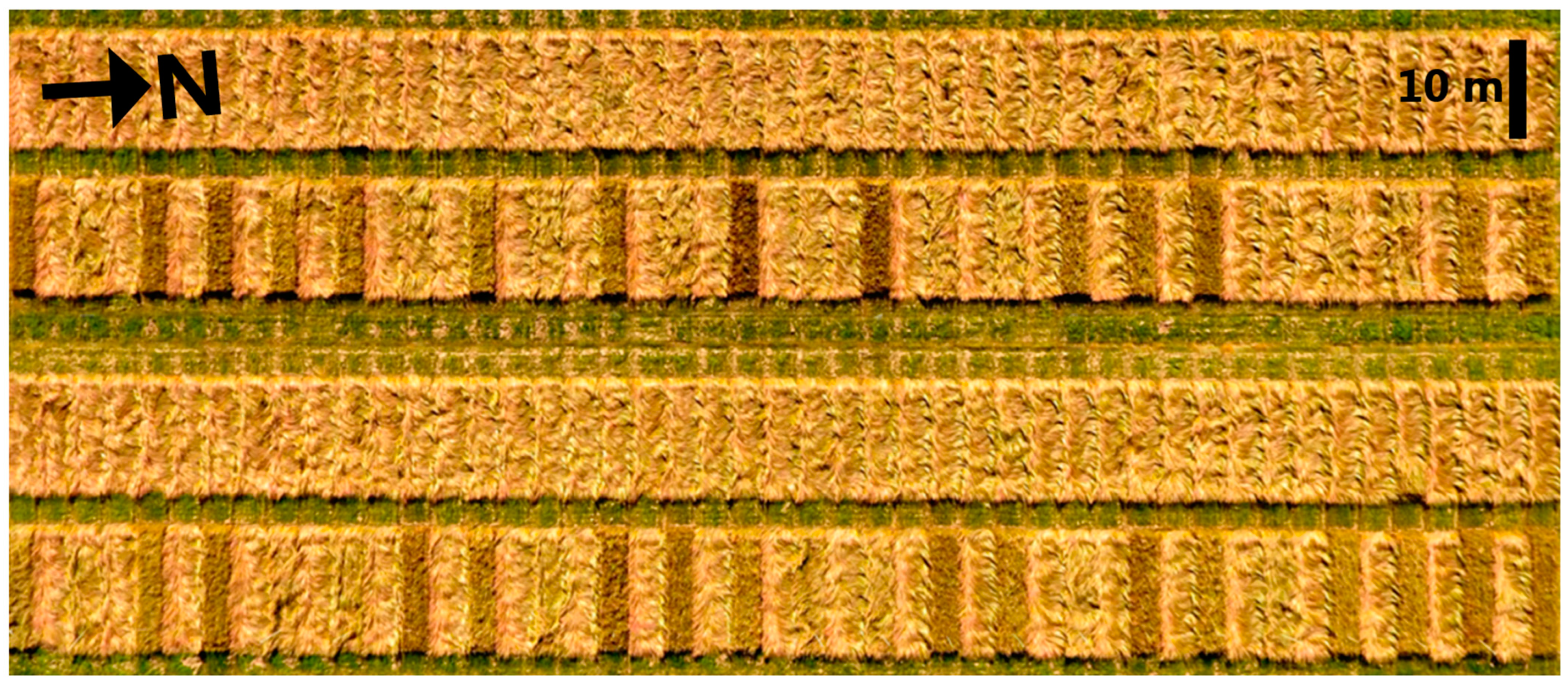
A 1.6 ha red fescue (cv. Maxima) field with clayey soil was established in 2018 at the research station of the University of Copenhagen in Taastrup (55°40′8.16″ N; 12°18′18.82″ E), Denmark. Red fescue was undersown in winter wheat (cv. KWS Lilli) the day after winter wheat establishment on 20 September 2018. Fertilizer and pesticide applications were used according to commercial farming practice to achieve the most profitable yield. Just before harvest in 2020, 20 plots distributed all over the fields were marked, representing large yield variation based on visual inspection of the field (
Figure 2).
The field was harvested on 14 July 2020 except for the marked plots, which were harvested on 1 August with a plot combine harvester. From each plot, the grass seeds were air-dried, and after cleaning, seed samples were weighed, and the weight converted to seed yield ha−1.
2.3. Drone Images
UAV images were captured with a Phantom 4 (DJI, Shenzhen, China) quadrotor equipped with a built-in GNSS and an integrated RGB camera before harvest on 27 June 2018 (
Figure 1) and on 17 July 2020 (
Figure 2). In 2020, UAV images were also captured before plots were marked on 3 March, 13 May, 26 May, and 24 June to investigate the importance of timing. On these dates, plots were identified after alignment with the 17 July orthomosaic where plots were visible.
Images were captured at noon +/− 2 h. Ground control points (GCPs) were used for geometric correction of orthomosaics. In each field, the position of ten visible markers were measured using Trimble R10 GNSS with TSC3 controller (Trimble, Sunnyvale, CA, USA). The positioning system receives correction signals from GPSnet.dk (Geoteam, Ballerup, Denmark), a Danish network of ground-based reference stations based on Trimble’s VRS technology (Trimble, Sunnyvale, CA, USA). This provided an accuracy of 0.02 m after post-processing.
The camera was a Sony 12.4 megapixel with a 1/2.3′ CMOS sensor (4000 × 3000 pixels). The flight altitude was 40 m according to onboard barometer measurements, and the ground sampling distance (GSD) was 1.7 cm pixel
−1. However, the precise flight altitude is considered of minor importance [
19]. Images were captured under stable light conditions. The frontal overlap of images with respect to the flight direction was 80%, and the lateral overlap was 70%. Average flight duration was 2.5 min ha
−1. Orthomosaics were generated in Pix4DMapper version 5.6.1, and plots were cropped from the orthomosaics with the open-source GIS software QGIS (
https://www.qgis.org/en/site/ (accessed on 17 January 2023)) version QGIS 2.18.1 Long Term Release (LTR), QGIS Development Team QGIS Geographic Information System. Open Source Geospatial Foundation Project (
http://qgis.org (accessed on 17 January 2023). The average size of orthomosaics was 120 MB per hectare. The spatial accuracy of created orthomosaics was less than 5 cm.
The mean values of the raw digital numbers of the red (R), green (G), and blue (B) bands for each plot were calculated in QGIS. There were no color calibrations.
2.4. Selection of Plots
The selection of plots for the training of the field-specific regression models was based on a combination of color variation in UAV photos and visual assessments of the crop yield on the ground to identify a wide range of crop yields. In 2018, the color variation in UAV photos constituted the selection criteria because there was a large variability in lodging. Lodging and color have previously been shown to correlate [
21], and it was assumed that yield and lodging were correlated based on visual inspections in the field. In 2020, selection of plots was based on visual yield inspections in the field. In 2018, 10, 20, and 48 plots were selected for training, and in 2020, 6 and 10 plots were selected for training to investigate the importance of an increasing number of plots used for training. Two criteria were used for the selection of training plots: (a) extreme VI values (the independent regression variable) and (b) random selection. A random selection was conducted to test the hypothesis that plots with extreme values of VI would increase the predictive power compared to a random selection of plots. The selection of random plots was repeated ten times for each number of training plots.
2.5. Vegetation Indices
We considered five vegetation indices (VI) based on the R (red), G (green), and B (blue) bands for the prediction models:
In addition to the five indices, the blue band (B) and the sum of R, G, and B were used as well. Mean values for each plot of the digital numbers (0–255) for R, G, and B were used in the calculations. Only results from the VI showing the strongest correlation between the index and the yield are presented (ExG [
22] and NGRDI [
23]).
2.6. Statistical Analyses
We used an increasing number of plots to train the field-specific linear regression models based on the two indices (ExG and NGRDI) to describe the relationship between the VI and the crop yield. The index obtaining the highest correlation was used to predict the yield, and the root mean square error (RMSE) was calculated to evaluate the predictive performance. RMSE reflects the average distance between the predicted yield and the actual yield and was calculated in absolute (kg ha−1) and relative terms (RMSE%). Predictions and RMSE were calculated for both training data sets and validated on the remaining part of the data sets. The minimum achievable RMSE was calculated based on regression analysis on the validation data sets. It reflected how well the validation data could be described by linear regression. Statistical analyses were conducted using the SAS® version 9.4 software (SAS Institute Inc., Cary, NC, USA). PROC CORR was used for correlation analysis and PROC GLM was used for parameter estimation and F-tests to evaluate the effect of training data set size on regression parameters. PROC GLM was used to calculate prediction intervals for any specific VI value. There is 95% probability that the real yield is within the calculated prediction interval for a specific VI value. The random selection of plots for training was carried out by using the UNIFORM function in SAS. The random selection was repeated ten times for each number of plots used for training.
3. Results
In 2018, the average yield was 1548 kg ha−1 with a standard deviation of 209 kg, and in 2020, the average yield was 1160 kg ha−1 with a standard deviation of 260 kg. Hence, the absolute and relative crop yield variation was larger in 2020.
ExG correlated slightly better with yield than NGRDI in 2018, whereas it was the opposite in 2020. When half of the plots were used for training (48 plots in 2018 and 10 plots in 2020), the correlation coefficients were 0.71 for ExG (
Table 1) and 0.69 for NGRDI in 2018. In 2020, the correlation coefficients were 0.77 for ExG and 0.80 for NGRDI (
Table 1).
Results did not support the hypothesis that the yield prediction accuracy was increased by using an increasing number of training plots. This was found when training was carried out on systematically selected plots (extreme values) (
Table 1) and randomly selected plots (
Table 2). In both years, parameters in the regression models based on extreme values were not statistically affected by the size of training data sets according to F-tests, which means that RMSE for predictions were more or less unaffected by the size of the training data sets (
Figure 3 and
Figure 4). However, the RMSE slightly increased in 2018 with the larger training set (
Table 1). A large training set means that the regression model was tested on medium yields only. The opposite trend appeared in 2020, where the largest RMSE were for the extreme yields (
Table 1). The minimum achievable RMSE in 2018 was 167 kg ha
−1, 172 kg ha
−1, and 190 kg ha
−1 when 10, 20, and 48 plots were used for training. In 2020, the minimum achievable RMSE was 137 kg ha
−1 and 127 kg ha
−1 when 6 and 10 plots were used for training.
In 2018, the selection criteria of test plots (extreme or random) were unimportant, if the benchmark for the randomly selected plots was average RMSE (
Table 1 and
Table 2). However, as indicated by the range of training correlation coefficients (
Table 2), there is a risk of poor yield prediction due to low correlations between yield and VI when training data is randomly selected. In 2020, the average prediction power based on models with randomly selected training data performed better than models training on extreme values (
Table 2).
The timing of the UAV image capture was unimportant in 2020 in weeks before harvest. The correlation between NGRDI and yield was 0.49 (p < 0.05), 0.68 (p < 0.001), 0.76 (p < 0.001), 0.79 (p < 0.001), and 0.77 (p < 0.001) on 3 March, 13 May, 24 May, 24 June, and 17 July, respectively.
4. Discussion
Trained local (field-specific) regression models based on UAV imagery showed to be a promising tool for generating yield maps. The yield predictions errors (RMSE) were in the range of 171 kg ha
−1 to 222 kg ha
−1 when training data sets consisted of 10 plots and training was based on extreme VI values (
Table 1). Different VI gave the best predictive power in different years (
Table 1). This was expected because yield variations may have different visual representations in different years and fields. For example, lodging may be negatively correlated with yield if it occurs early in the growing season before pollination [
21]. In 2018, lodging showed clearly visible effects in UAV images (
Figure 1), whereas it played a minor role in 2020 (
Figure 2). Lodging may also be positively correlated with yield if it occurs late in the growing season because of heavy fertile tillers. In 2020, soil fertility had an impact on the greenness of the crop throughout the growing season, which was expressed in NGRDI.
In 2020, the exact timing of UAV image capture was shown to be unimportant in the weeks before harvest because yield variation was related to general growth conditions in the field. The underlying mechanism was possibly caused by soil fertility because crop growth variation was visible throughout the growing season. Therefore, it was possible to establish a significant correlation (p < 0.05) between NGRDI and yield in the early spring (3 March 2020). UAV imaging throughout the growing season can be helpful to obtain an understanding of why and when lodging has taken place. It may indicate whether lodging is caused by high yields or heavy rainfall, or insufficient application of plant growth regulators before the pollination had taken place, resulting in a potential low yield, or perhaps a mixture resulting in site-specific variations.
The basic idea of this study was to train regression models based on extreme VI values, but the results showed that random selection of data might provide similar or even better results. With random selection, however, there is a risk of poor correlation between VI and yield (
Table 2), leading to poor predictions (
Table 2). In 2018, the predictions were close to optimum for the suggested prediction method based on extreme values, because RMSE approached the minimum achievable RMSE values. In 2020, selection of plots covering the whole range of VI would probably have been better because RMSE values were significantly greater than the minimum achievable RMSE and because random selection of plots for training showed lower RMSE. Therefore, the results indicate that it is not necessary only to use extreme values.
The study showed that there is no general relationship between canopy color and yield between fields, and consequently, there is no general relationship between a specific VI and yield. This calls for local models based on field-specific training. Yield predictions based on remote sensing have been investigated thoroughly [
24]. Still, the experimental approach in our study differs from the majority of the previous studies [
25,
26,
27,
28], which investigated advanced machine learning algorithms to make out-of-sample predictions (global models). This means that field-specific training can be avoided in opposite to the approach presented in our study. This may appear as an important advantage, but from an applied perspective, local models may have one significant advantage compared to global automated algorithms: robustness.
Furthermore, global models do not currently exist and there are no indications that such models will be developed in the foreseeable future. As a result, the only practical way to generate yield maps using prediction models is currently by implementing models that are trained specifically for each field. The training aspect is not necessarily a decisive barrier for implementation. Rasmussen et al. [
29] approach for detecting and mapping thistles (
Cirsium arvense L.) based on a local trained model was successfully integrated into Danish farmers’ CropManger IT-platform (
https://cropmanager.dk/ (accessed on 17 January 2023)). Like for thistle detection, there will be preconditions that need to be met for reliable yield predictions. Clear correlation between yield and colors in drone images must exist. This will not be the case if the yield variability within a field might be a result of different causes giving different spectral signatures. If lodging is determining yield in some part of the field as in the 2018 experiment, and general growth conditions are determining yield in other parts of the field as in the 2020 experiment, the presented regression approach may fail. Therefore, the regression approach has its limitations, but future studies or practical experiences will have to show whether these limitations are crucial. The limitations of the regression approach depend largely on the nature of the variability, which occurs in grass seed fields. The nature and the extent of this variability has not been studied yet.
In a practical perspective, the cost of training local models must be considered. The main challenges are to obtain reliable yield data from contrasting yield environments and to match plots on ground and in UAV mosaics and to identify a VI that correlates with yield. UAV image acquisition is a prerequisite for both global and local models. It is hardly likely that farmers themselves will undertake all work tasks, which indicates that yield maps based on UAV imagery most likely must be produced by service providers or research institutions. Whether farmers are willing to pay for yield maps is beyond the scope of this article, but it could be argued that yield maps in grass seed crops at present is primary relevant for experimental purposes.


