Abstract
A full understanding of the growth and distribution of tree roots is conducive to guiding precision irrigation, fertilization, and other agricultural work during agricultural production. Detecting tree roots with a ground-penetrating radar is a repeatable detection method that does no harm to the earth surface and tree roots. In this research, a rapid and accurate automatic detection was conducted on hyperbolic waveforms formed by root targets in B-scan images based on YOLOv5s. Following this, the regions of interest containing target hyperbolas were generated. Three or more coordinate points on the hyperbola were selected according to the three-point fixed circle (TPFC) method to locate the root system and estimate the root diameter. The results show that the accuracy of hyperbola detection using YOLOv5s was 96.7%, the recall rate was 86.6%, and the detection time of a single image was only 13 ms. In the simulation image, the TPFC method was used to locate the root system and estimate the root diameter through three different frequency antennas (500 MHz, 750 MHz, and 1000 MHz). A more accurate result was obtained when the antenna frequency was 1000 MHz, with the average distance error of root system positioning being 3.17 cm, and the slope and of the linear fitting result between the estimated root diameter and the actual one being 1.029 and 0.987, respectively. Verified by the pre-buried root test and wilderness field test, both root localization and root diameter estimation in our research were proved to gain good results and conform to the rules found in simulation experiments. Therefore, we believe that this method can quickly and accurately detect the root system, locate and estimate the root diameter, and provide a new perspective for the non-destructive detection of the root system and the three-dimensional reconstruction of the root system.
1. Introduction
The roots of trees can not only take in water and nutrients for the plants but also serve as the trees’ mechanical support [1,2]. Efficient and non-destructive in situ quantitative detection and study of root morphology, functional structure, and distribution characteristics can provide accurate irrigation and fertilization of trees and improve resource utilization. At the same time, during agricultural production, it is necessary to understand the growth and development of trees and to provide guidance for root health monitoring of trees [3,4]. By the traditional root detection methods, such as excavation method and soil auger method, plant roots and soil environment can be damaged, and a long-term and repeatable detection and research cannot be carried out on the root system [5]. However, by using some detection techniques that cause little or no destruction, such as micro-root window tube method, nuclear magnetic resonance imaging, X-ray tomography, capacitance method, and resistivity imaging technique, the detections can only be conducted within a small range and are very possibly limited by field conditions [6,7,8,9].
Compared with the above techniques, the ground-penetrating radar (GPR) is increasingly being applied to the nondestructive detection of plant roots at home and abroad due to its advantages of causing no destruction to the ground surface and the tree’s root system, as well as its wide detection range and conduciveness to performing repeatable tests at the same location [10,11,12]. According to the research by Yamase et al. [13] on using GPR to estimate the diameter of coarse plant roots in the forest field, the detection rate of root diameter that is greater than 5 mm was 47.7%, and the root diameter size and the root depth would affect the accuracy of detection. The manual detection of targets from B-scan images is often time consuming and somewhat subjective, and thus the automated detection of hyperbolas formed by root targets is of great significance to our research [14]. The traditional methods for automatic detection of targets include the Hough transform method and least squares method [15]. Li et al. [16] used the stochastic Hough transform algorithm based on the GPR dataset from the control experiments and in situ experiments in order to identify root targets detected at different antenna frequencies, with an accuracy of about 80% and a false alarm rate of less than 1.5/m. There are some deficiencies in traditional target detection methods: for example, a large amount of computation is required, and simultaneous detection of multiple targets cannot be conducted. Many scholars tried detecting target hyperbolas through combining machine learning methods. Maas et al. [17] used the VJ (Viola–Jones) algorithm to reduce the computational amount by narrowing the target hyperbolas region so as to reduce the Hough transform input amount. However, the quality of the detection results depends largely on the quality of the training samples. Wang et al. [18] proposed a semi-automatic detection method based on the genetic algorithm to identify buried steel bars in GPR data, whose average false positive rate and missed detection rate were 9.08% and 11.98%, respectively, and decreased with the gradual increase in the antenna frequency. In recent years, the deep learning technology has been widely used for automatic detection of target features in GPR scanned images [19,20,21]. Pham et al. [22] used Faster-RCNN for target detection of B-scan images of GPR, but the training samples were mainly from the simulated images created by GprMax simulation software, and there was insufficient quantity of real image samples. Hou et al. [23] used the MS R-CNN (mask scoring R-CNN) framework to detect the target while solving the problem of insufficient quantity of training samples by migration learning.
A synthesis of previous studies revealed that the detection of target hyperbolas using manual methods is often laborious and somewhat subjective. Traditional automatic target detection methods and machine learning methods lack a high degree of automation or tend to have increasingly limited detection capability as the amount of data increases. To address these problems, this paper proposes a deep learning and ground-penetrating-radar-based method for root localization and root diameter estimation. YOLOv5s was selected as the detection model to frame the target hyperbola in B-scan images, and the root system localization and root diameter estimation were conducted by the three-point fixed circle (TPFC) method.
2. Materials and Methods
2.1. GPR Detection Methods and Imaging Principles
Generally speaking, the root system grows towards all directions in a radial way with the tree stump as its center. In order to maintain an as-perpendicular-as-possible detection direction of the ground-penetrating radar to the growth direction of the root system for more accurate detections, several concentric circles with equal spacing were selected as the detection route of the ground-penetrating radar for tree root detection, and its schematic diagram is shown in Figure 1.
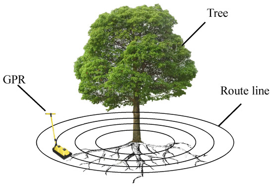
Figure 1.
Detection method.
The principle of GPR imaging is shown in Figure 2. The left figure shows the cross-sectional view of GPR root detection, while the right figure shows the ground-penetrating radar detection process, in which high-frequency pulses are sent and echoes are received at every segment distance to obtain A-scan data. Multiple A-scan data are stacked to form two-dimensional cross-section echo data, namely, B-scan. As shown in the middle figure, the vertical axis of B-scan is based on the dual travel time, i.e., the time length starting from sending a high-frequency pulse to receiving its echo, while the number of A-scan channels is shown on the horizontal axis, and the distance between two adjacent A-scan channels is the channel spacing, i.e., the forward progress length of GPR detection. The GPR detection was conducted from far to near distance and then from near to far distance, so as to present a hyperbolic wave with a downward opening in the B-scan.
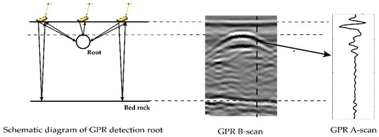
Figure 2.
GPR imaging principle.
2.2. Model Training
2.2.1. Data Pre-Processing
The dataset used for the deep learning network model training was divided into real measurement images and simulation images. Among 2069 total images, there were 997 real images and 1071 simulated ones. According to the ratio of 4:1, the dataset was divided into the training set and testing set. The data set was manually labeled using LabelImg software, with the labeling method shown in Figure 3. For the hyperbola framing, the hyperbola’s vertices were placed in the middle of the rectangular box to enclose the whole hyperbola as much as possible, and a label file was generated corresponding to the image after the hyperbola framing is completed. The red area indicates the framed hyperbola that needs to be labeled, while the yellow area indicates that the label was not generated because the hyperbola was blurred or there was only a small part of the hyperbola waveform.
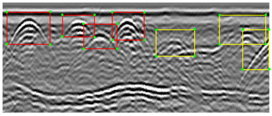
Figure 3.
Schematic diagram of hyperbolic labeling. The red area indicates the framed hyperbola that needs to be labeled, while the yellow area indicates that the label was not generated because the hyperbola was blurred or there was only a small part of the hyperbola waveform.
2.2.2. YOLOv5s Network Model
The YOLO (You Only Look Once) series of algorithms belong to the single-stage target detection algorithms. They have evolved to the YOLOv5 series, which is more efficient and lighter in terms of detection speed and accuracy compared to the previous versions [24], and the YOLOv5 network has a total of four versions: x, l, m, and s, whose weights, model depth, and width are increased sequentially. Due to the relatively simple shape and color of the target to be detected, the YOLOv5s model that is smaller and faster was chosen as the detection model in the study. The entire network structure of YOLOv5 consists of four parts: the input layer, backbone network, connection network, and output layer, with its structure shown in Figure 4. First, the input image was resized to be in 640 × 640 pixels, and the Mosaic data enhancement was performed at the input side. Then, the slicing operation was performed at the Focus layer in the backbone network, followed by the feature extraction through a series of cross stage partial (CSP) structures, and spatial pyramid pooling (SPP) was used to fuse more features of different resolutions to obtain more information. The multi-scale fusion of features was developed by combining the feature pyramid network (FPN) and path aggregation network (PAN) in the connection network. At the output side, GIOU_Loss was used as the loss function to obtain 17 × 17, 20 × 20, and 23 × 23 feature maps at different scales through different convolutional layers in the network for the final successful target detection.
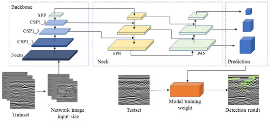
Figure 4.
YOLOv5s network structure diagram.
2.2.3. Model Evaluation Indicators
Following the model training, the Precision (P) and Recall (R) of the model in the test set were used as the precision evaluation metrics. Precision is the proportion of samples that are proved to be positive in the actual evaluation in all samples predicted to be positive. Recall is the proportion of all samples that are predicted to be positive in all samples that are proved to be positive in the actual evaluation. The calculation of these metrics is shown in the Equations (1) and (2). The average detection time is used as the index of evaluating the detection speed, and its calculation formula is shown in Equation (3).
where TP is the positive samples correctly predicted by the model, FP is the negative samples incorrectly predicted as positive by the model, FN is the positive samples incorrectly predicted as negative by the model, is the time required to detect all images in the test set (in ms), and is the number of images in the test set.
2.2.4. Experimental Environment and Parameter Settings
The computer used to train the model included the Windows10 operating system with an Intel (R) Xeon (R) Gold 6240 CPU@2.60 GHz with 36 cores, with a 2TB solid state drive. The graphics card was a dual-channel Nvidia GeForce GTX 3090, and the GPU memory was 48 GB. The programming language used to implement the model was Python3.8, and the training was based on the PyTorch deep learning framework, version 1.8. The unified computing device architecture was CUDA11.3.
Transfer learning is used to improve the training speed of the model. The batch size was set to 8, the number of training epochs was 200, the input image size was uniformly adjusted to 512 × 512, the initial learning rate was 0.001, the initial learning rate momentum was 0.937, and the weight attenuation coefficient was 0.0005; Adaptive Moment Estimation (ADAM) was used as the optimizer for model training.
2.3. Root System Localization and Root Diameter Estimation Using the TPFC Method
2.3.1. Principle of TPFC Method
The main principle of the three-point fixed circle (TPFC) is as follows: at least three sampling points were selected in the GPR detection process—these sampling points needed to be located on the same measuring line, which had to be as perpendicular as possible to the root growth direction. Then, the geometric relationship between the sampling points and the root target was applied to locate and estimate the root diameter [25]. The principle of the TPFC method is shown in Figure 5, where three or more equations can be derived on the basis of the horizontal position of the selected sampling points, the two-way travel time of the electromagnetic waves, and the geometric relationship among the root target. This set of equations can be used to calculate the coordinates of the coarse root and its radius, whose system of equations is shown in Equation (4).
where is greater than or equal to 3; , are the coordinates of the center of the coarse root; and are the vertical heights of the probe points. When the detection mode of GPR is a horizontal one that is conducted close to the ground, it is believed that , where is the radius of the coarse root and are the distances from the three detection points to the wall of the root system, respectively. Figure 6 is the diagram displaying the TPFC method, with the horizontal coordinates representing the number of acquisition channels and the vertical coordinates representing the two-way travel time of the electromagnetic wave. When the two-way travel time and the distance from the sampling point to the wall of the root system satisfies and the coordinate information of the sampling point is substituted into Equation (4), we can obtain
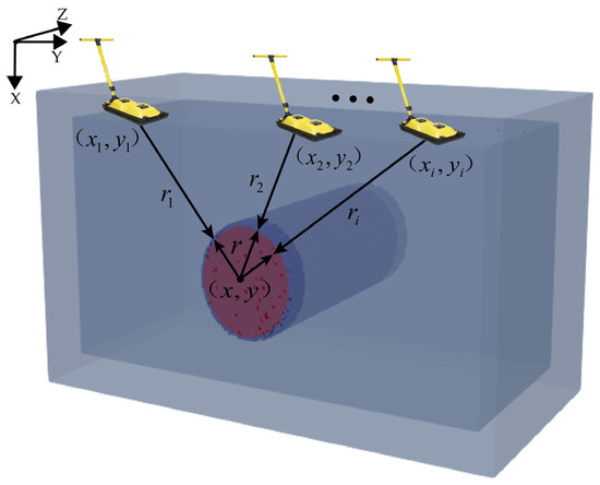
Figure 5.
TPFC method schematic diagram.
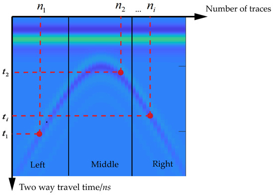
Figure 6.
Select coordinate point.
B-scan consists of several A-scan traces. In the Equation (5), refers to the trace spacing in the unit of m, , , … indicates the number of acquisition traces that is also the serial number of A-scan, … indicates the two-way travel time of electromagnetic waves in the unit of ns, and is the propagation speed of electromagnetic waves in the soil medium in the unit of m/s. The calculation formula is
where is the propagation velocity of electromagnetic waves in vacuum, and its value is about m/s, and is the relative dielectric constant of the medium. Combining with Equation (6), Equation (5) can be transformed into
The number of equations in Equation (7) is greater than the number of unknowns and can be calculated iteratively using the Levenberg–Marquardt algorithm to solve for the , , optimal solutions, i.e., the central location of the roots as well as the root diameter [24].
2.3.2. Experimental Design
- Simulation test
During the root localization experiment using the simulation data created by GprMax 2D, the specific parameters of the simulation model were set by writing an input file. The size of the simulation space range was set to be 3 × 0.8 , and the time window was set to 10 ns. Set according to those of dry sandy loam, the relative permittivity of the soil medium parameters was set to be 3, its relative permeability was 1, and its conductivity was 0.001 S/m. Since dry sandy soil is a non-ferromagnetic substance, its relative permeability was 1. The movement step of the antenna was set to be 0.02 m, the depth of the root was controlled within 0.5 m, the distance between adjacent roots was 0.5 m, the root diameter was set to 2 cm, and the relative dielectric parameter of the roots was set to be 20. The effects of different antenna frequencies (500 MHz, 750 MHz, 1000 MHz), different root depths, and different root diameters on root localization and root diameter detection results were quantitatively analyzed.
In the root diameter detection experiment, the range size of the simulation space, the parameters of the soil medium, and the dielectric constant of the roots were kept the same as those in the previous experiment, while the diameter of the roots was selected from 0.5 to 8 cm, and the depth was set at 20 cm.
- 2.
- Pre-buried root test
In order to verify the feasibility of applying the method proposed in this paper in actual detection, the PulseEKKO PRO ground-penetrating radar produced by the Canadian Sensor&Software Company was used in the soil trough laboratory of the Engineering College of South China Agricultural University to conduct a pre-burial test under controlled conditions. The size of the soil tank was 8 2 1.5 . The soil type of dry sandy loam has evenly distributed and stable physical properties that can be simulated easily to avoid the formation of clumps and voids by the reflection images of the ground-penetrating radar. According to the results of the simulation test, it can be found that when the antenna frequency was 1000 MHz, the results of positioning and root diameter estimation were more accurate than those by using antennas with two other different frequencies. Therefore, the antenna frequency of GPR was chosen to be 1000 MHz in the root pre-burial test. Fresh branches with relative dielectric constants close to those of the roots were selected as the test materials. There are two kinds of experiments under different experimental conditions. The first one targets the tree roots with same diameter buried at different underground depths, as shown in Figure 7a. Five branches with close diameters, numbered 1 to 5, were selected for the experiment, whose diameters ranged from 26 to 28 mm. They had a spacing of about 30 cm between their adjacent branches. They were buried underground at a depth ranging from 10 to 50 cm with each buried with a depth difference of about 10 cm. The second kind of experiment targets the tree roots with different diameters buried at the same underground depth, as shown in Figure 7b. Five branches of different diameters, numbered 6 to 10, were selected for the experiment. Their diameters ranged from 0.5 to 8 cm, and the spacing between their adjacent branches was 50 cm. They were buried at an underground depth of 20 cm. Before the detection of roots starts, it is necessary to measure the propagation velocity of electromagnetic waves in the soil. Since the physical properties of the soil in the soil tank remain stable and evenly distributed, the velocity of electromagnetic waves can be calculated according to the propagation theory of electromagnetic waves when the depth of the target object is known [26], The formula is shown in Equation (8).
where is the propagation speed in the electromagnetic wave soil, is the depth of the target object, and is the two-way travel time of the electromagnetic wave.
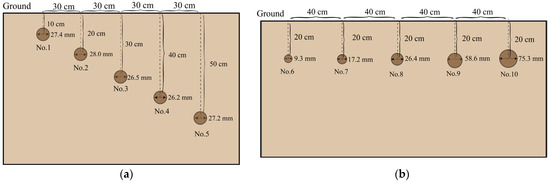
Figure 7.
Schematic diagram of pre-buried root test: (a) different depth; (b) different root diameters.
- 3.
- Field test
In order to further verify the feasibility of the method proposed in this paper, field detection experiments were conducted in the woods near the College of Engineering, South China Agricultural University, Guangzhou (113°28′06″ E, 23°12′51″ N). The test subject was Bauhinia. The equipment used in the test was the pulseEKKO PRO ground-penetrating radar, and the center frequency of the antenna was 1000 MHz. The GPR detection route is shown in Figure 8a, being eight concentric circular tracks centered on the tree in total, with the innermost detection route being 30 cm from the center of concentric circle and the spacing of adjacent routes being 15 cm. The starting point of each detection route and the center of concentric circle were on the same straight line. Each detection route was repeated three times. In order to alleviate the damage to the tree, only a quarter of the detection area was excavated for result verification, and the excavation depth was 40 cm, as shown in Figure 8b. Then, the root nodes on the detection route were marked and numbered, and the depths, diameters, and coordinate positions were measured. In the vicinity of the test object, a target object was buried at a depth of 30 cm and detected by GPR, as shown in Figure 9. When its two-way travel time was recorded, the electromagnetic wave velocity was determined according to the electromagnetic wave velocity determination method mentioned in Section 3.2.2.
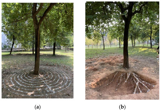
Figure 8.
Field test: (a) detection route; (b) root excavation for verification.
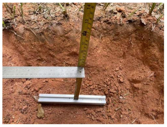
Figure 9.
Field electromagnetic wave velocity measurement.
2.4. Root System Localization and Root Diameter Estimation Method for Trees Using Ground-Penetrating Radar
On the basis of the above methods and principles, a new method was proposed in this paper for root localization and root diameter estimation of trees using GPR, and the complete implementation process is shown in Figure 10:
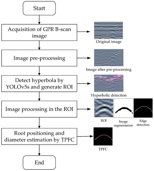
Figure 10.
Implementation process of the method.
- Acquisition of B-scan image data collected by ground-penetrating radar, whose specific steps are shown in Section 2.1.
- Image pre-processing. Its main purpose is to reduce the noise related information in the ground-penetrating radar data, and its main operations include zero correction, background removal, and image gain and filtering [27,28], with the related operations mainly completed on EKKO_Project4 software and MATLAB. In the zero correction, the time point was calibrated when the electromagnetic wave emitted from the radar antenna reached the ground; in the background removal, the mean reference value was gained by subtracting the background noise date from all B-scan trace data. The image gain mainly adopted automatic gain and spherical wave index compensation, and the image filtering mainly refers to Gaussian filtering, etc.
- The trained YOLOv5s were used to detect the target hyperbolas in the B-scan images, which generated the region of interest (ROI) containing only one root target hyperbola, and sent back the coordinate information of the target borders. The specific training method is shown in Section 2.2.
- The image was processed within the region of interest to extract the feature information of the hyperbolas. Its main operations include image clustering, image segmentation, and edge detection [29]. Image clustering was to cluster independent hyperbolas and separate the intersecting hyperbolas using the column connection clustering (C3) algorithm [30] proposed by Dou et al. Image segmentation refers to the binarized image segmentation using the OSTU algorithm, and after the segmented image was obtained, the Canny operator or Sobel operator was used to perform edge detection on the segmented image.
- After three or more coordinate points on the hyperbola were selected, the center point (x, y) of the root was located and the root diameter was estimated using the TPFC method, as shown in Section 2.3.
Through the above steps, the tree root system was localized, and the root diameter was estimated.
3. Results
3.1. Experimental Analysis of Root Detection Based on YOLOv5s
The detection results by this model on the validation set are shown in Figure 11a, where all the root target hyperbolas can be framed with a confidence level of 0.92 or even higher. Figure 11b shows the variation of the accuracy and recall rate of using the model in 200 epochs, with the accuracy rate reaching 96.7% and the recall rate 86.6%. It is obvious that the accuracy rate is rather satisfactory, while there is still some room for improvement in the recall rate. The average detection time per image was 13 ms, which is much less than the time required for manual detection. All these results show that the YOLOv5s model can be used to detect the hyperbola of objects in B-scan images quickly and accurately.
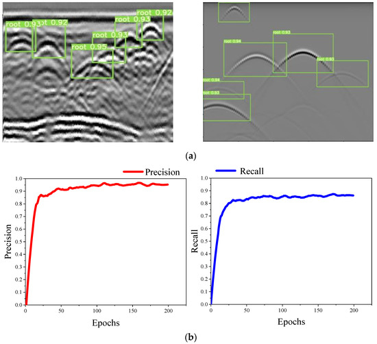
Figure 11.
YOLOv5s results: (a) YOLOv5s detection results; (b) change curve of the evaluation index of using the YOLOv5s model.
3.2. Root System Localization and Root Diameter Estimation Results
3.2.1. Simulation Test Results
The simulation model and results are shown in Figure 12a,b.
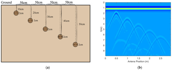
Figure 12.
Simulation results at different depths: (a) simulation model; (b) simulation image.
The experimental data were recorded and organized using Excel 2019 and graphically plotted using Origin 2021. The experimental results of root localization are shown in Table 1. Overall speaking, when the depth was less than 50 cm, the distance error for root localization using this method was kept within 5 cm, and the average distance errors were 3.93 cm, 3.49 cm, and 3.17 cm each when using three different frequency antennas. At the frequency of 1000 MHz, the distance error was the smallest, and when the frequency was 500 MHz, its distance error was relatively larger, which indicates that different antenna frequencies had certain effects on the distance error of root localization. The higher frequency of the ground-penetrating radar antenna will lead to more accurate results of root localization using the TPFC method.

Table 1.
Root location results.
The simulation model and results are shown in Figure 13a,b, respectively. The results of the root diameter estimation in the TPFC method using GPRs with three different frequency detection antennas (500 MHz, 750 MHz, and 1000 MHz) are shown in Table 2. The linear fit of the root diameter estimation results is shown in Figure 14.
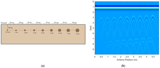
Figure 13.
Simulation of different root diameters: (a) simulation model; (b) simulation image.
Table 2.
Root diameter estimation results.
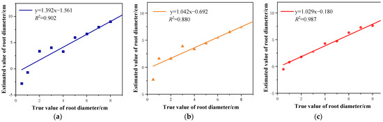
Figure 14.
Linear fitting of root diameter estimation results: (a) estimated root radius at an antenna frequency of 500 MHz; (b) estimated root radius at an antenna frequency of 750 MHz; (c) estimated root radius at an antenna frequency of 1000 MHz.
For root diameters greater than 1 cm, the estimates were very close to the actual values, with the slopes of the fits being 1.392, 1.042, and 1.029, and s being 0.902, 0.880, and 0.987. It can be seen that the root diameter estimation result was closest to the real value at the antenna frequency of 1000 MHz. The relative errors of the estimation results are compared in Figure 15. Under these three circumstances, the maximum value of the relative error was obtained at the minimum value of the root diameter, and the relative error gradually decreased with the increase in the root diameter. The relative error of root diameter estimation by using the 1000 MHz radar antenna was smaller than that using other two antennas, which was kept within 10% for root diameters greater than 2 cm. These results demonstrate the feasibility of estimating the root diameter of trees using the TPFC method.
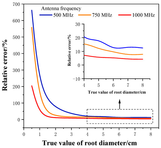
Figure 15.
Change of relative errors of root diameter estimation.
According to the results of root localization and root diameter estimation by TPFC method in the simulation test, it can be seen that there were rather small margins of errors in the root localization and root diameter estimation at 1000 MHz antenna frequency, but in the specific application, not only should the appropriate antenna frequency be selected according to the depth of the detection target, but also the electromagnetic characteristics of the underground medium and the diversity of the measured environment should be considered.
3.2.2. Pre-Buried Root Test Results
The test results on the pre-buried root are shown in Table 3. It can be seen from the root number 1~5 in the table that the distance error of root localization detection results was kept within 6 cm. In other words, the higher depth would cause a greater distance error. For the branches with different diameters, their roots were numbered from 6 to 10. When their diameters were less than 1 cm, there were larger relative errors in their diameter estimation results, and the figure decreased accordingly as the root diameter increased. Overall speaking, satisfactory results were achieved in root localizations and root diameter estimations. However, there were still relatively larger margins of errors compared with those in the simulated experiments, as the results may have been affected by clutter waves generated due to different soil densities caused by uneven compaction during the soil filling, or because the relative permittivity of the roots that is not very different from that of the soil resulted in less obvious hyperbolic features.
Table 3.
Pre-buried root test results.
In summary, the results of the simulation and pre-buried root tests prove the feasibility of the TPFC method for root localization and root diameter estimation. In the real-scene field test, excavation and measurement is required after root detection is completed, and then the detection effect can be analyzed.
3.2.3. Field Test Results
The B-scan images obtained from ground-penetrating radar detection were pre-processed, and the operation procedure was referred to Section 2.4, with the pre-processed results shown in Figure 16.
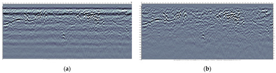
Figure 16.
Image pre-processing: (a) before image pre-processing; (b) after image pre-processing.
In the field test, a total of 70 root nodes were marked, among which there were 48 root nodes with root diameter above 1 cm. There were 42 hyperbolic waveform targets on B-scan images, and 37 hyperbolic waveform targets were successfully detected by the YOLOv5s detection model, with a detection rate of 88.09%. This indicates that the detection model based on YOLOv5s had a high detection rate for hyperbolic waveform in B-scan images detected in the field. From the results in Table 4, it can be seen that the maximum error of diameter estimation was 34.18% and the minimum error was 6.83%. The minimum and maximum distance between the predicted position of root positioning and the actual position were 0.67 cm and 8.73 cm, respectively. The error of root location and diameter estimation in the inner circle was larger than that in the outer circle. When the root diameter was small, the error of the root diameter estimation results was large, which is consistent with the test results on the simulation diagram, indicating that the method proposed in this paper had a certain feasibility in the field test.
Table 4.
Pre-buried root test results.
4. Discussion
4.1. Discussion on Root Detection Test Results Based on YOLOv5s
The test results of root detection based on YOLOv5s show that the hyperbola in a B-scan image can be quickly detected by YOLOv5s with a high confidence coefficient and accuracy. Compared with the detection methods based on mathematical models or machine learning, as well as traditional manual detections, the method of deep learning used in our research in this paper has greater advantages in detection accuracy and speed [31,32,33], but there is still some room for improvement, such as improving the quality of data samples or further optimizing the model structure to improve the performance of the network model.
4.2. Discussion on Root Positioning and Root Diameter Estimation Results
The antenna frequency of GPR has a direct relationship with the results of root localization and root diameter estimation. The higher antenna frequency means the higher resolution, which will lead to more accurate root localization. This is because the higher the antenna frequency of the ground-penetrating radar, the higher its spatial resolution. In addition, the electromagnetic wave emitted by the antenna with a high frequency has more concentrated energy and better direction, and thus the echo intensity of the electromagnetic wave is better, presenting a clearer and more accurate hyperbola in the B-scan of a ground-penetrating radar. In the TPFC method, the more accurately the sampling points can be obtained, the more accurate the estimation results will be. However, the detection depth of the antenna with a high frequency will be relatively low, and the noise and clutter in the detection image will increase correspondingly, which may bring about more challenges to image processing. Therefore, in practical applications, the appropriate antenna frequency should be selected according to the depth of the detection target. During the propagation of electromagnetic waves in the soil, its energy will gradually decay, thus affecting the definition of hyperbola waveform in a B-scan image. The definition of the hyperbola has a significant impact on whether accurate sampling points can be obtained in the TPFC method. The deeper the depth is, the more blurred the hyperbola formed by the target echo may be, resulting in the failure to obtain accurate sample points in the TPFC method, which will affect the estimation result with greater error. For roots with small diameters, their upper and lower surfaces cannot be distinguished due to the vertical resolution of the GPR, resulting in the failed B-scan images of their hyperbolas [27].
In the pre-buried root test, overall speaking, satisfactory results have been achieved in root localizations and root diameter estimations. However, there were still relatively larger margins of errors compared with those in the simulated experiments, as the results may have been affected by clutter waves generated due to different soil densities caused by uneven compaction during the soil filling, or because the relative permittivity of the roots that is not very different from that of the soil resulted in less obvious hyperbolic features.
The results of the field test show that the proposed method is also somewhat credible in field conditions, but there are still inadequacies in this field test. First, the horizontal angle of a root crossing a scanning line is a factor that affects both root detection and waveform parameter values [34]. The large angular variation of the detection direction during the inner circle detection resulted in the distortion of the hyperbola presented on the B-scan. Secondly, the reflected waves of the roots close to the surface are easily affected by the ground waves, resulting in the failure in taking B-scan images of some roots located at the surface. In addition, the heterogeneous soil texture and the presence of other foreign materials in the soil also bring some challenges to field detection.
5. Conclusions
This paper proposes a method based on YOLOv5s and ground-penetrating radar technology to realize the fast and accurate detection of hyperbolas in B-scan images, with the TPFC method applied to accurately locate and estimate root diameters. This study quickly and accurately detected root systems and performed localization and root diameter estimation, providing some ideas for nondestructive root detection and three-dimensional reconstruction of root systems. However, there are some problems and inadequacies that need to be solved in future work. First, due to the complex soil environment, complexity of field tests and the inability to distinguish whether the collected data are those of roots or other foreign objects, further research is needed to investigate the differences in hyperbolic characteristics between roots and non-root targets. Secondly, further research is needed on the removal of clutter and methods to enhance the hyperbolic signal.
Author Contributions
Conceptualization, D.S., F.J., H.W. and Z.Z.; methodology, F.J., H.W., S.L. and P.L.; software, F.J., H.W. and P.L.; validation, F.J., D.S. and H.W.; formal analysis, F.J., S.L. and H.W.; investigation, D.S., F.J., H.W., S.L., P.L. and Z.Z.; resources, D.S. and Z.Z.; writing—original draft preparation, F.J.; writing—review and editing, D.S.; visualization, F.J., H.W. and P.L.; supervision, D.S.; project administration, D.S. and Z.Z.; funding acquisition, D.S. and Z.Z. All authors have read and agreed to the published version of the manuscript.
Funding
This research was funded by State Key Research Program of China “Research on testing method of machine operating state parameters” (no. 2016YFD0700101-02). It was also partly supported by the Guangzhou Science and Technology Plan Project (no. 202002030245); the Guangdong Provincial Organization of China and the implementation project in 2021 (YUECAINONG no. 37) entitled “Integration and Demonstration of Key Technology Models of Modern Agriculture in Guangdong Province”; the special fund for the innovation team construction of the modern agricultural industrial technology system in Guangdong Province (no. 2022KJ108); the 2020 special fund for science and technology innovation strategy of Guangdong Province (special fund for “climbing plan”, no. pdjh2020a0084); and the Guangdong University Student Innovation and Entrepreneurship Project (no. S202010564150, no. 202110564042, no. X202110564140).
Data Availability Statement
The data presented in this study are available on request from the corresponding author. The data are not publicly available due to the privacy policy of the organization.
Conflicts of Interest
The authors declare no conflict of interest.
References
- Lynch, J.P. Root Phenotypes for Improved Nutrient Capture: An Underexploited Opportunity for Global Agriculture. New Phytol. 2019, 223, 548–564. [Google Scholar] [CrossRef] [PubMed]
- Zhang, L.; Cui, X.; Quan, Z. Availability of ground penetrating radar in recognizing plant roots in field. Prog. Geophys. 2021, 36, 2764–2774. [Google Scholar]
- Cabal, C.; De Deurwaerder, H.P.T.; Matesanz, S. Field Methods to Study the Spatial Root Density Distribution of Individual Plants. Plant Soil 2021, 462, 25–43. [Google Scholar] [CrossRef]
- Zhang, X.; Derival, M.; Albrecht, U.; Ampatzidis, Y. Evaluation of a Ground Penetrating Radar to Map the Root Architecture of HLB-Infected Citrus Trees. Agronomy 2019, 9, 354. [Google Scholar] [CrossRef]
- Molon, M.; Boyce, J.I.; Arain, M.A. Quantitative, Nondestructive Estimates of Coarse Root Biomass in a Temperate Pine Forest Using 3-D Ground-Penetrating Radar (GPR). J. Geophys. Res.-Biogeosci. 2017, 122, 80–102. [Google Scholar] [CrossRef]
- Alani, A.M.; Lantini, L. Recent Advances in Tree Root Mapping and Assessment Using Non-Destructive Testing Methods: A Focus on Ground Penetrating Radar. Surv. Geophys. 2020, 41, 605–646. [Google Scholar] [CrossRef]
- Weigand, M.; Kemna, A. Multi-Frequency Electrical Impedance Tomography as a Non-Invasive Tool to Characterize and Monitor Crop Root Systems. Biogeosciences 2017, 14, 921–939. [Google Scholar] [CrossRef]
- Shamir, O.; Goldshleger, N.; Basson, U.; Reshef, M. Laboratory Measurements of Subsurface Spatial Moisture Content by Ground-Penetrating Radar (GPR) Diffraction and Reflection Imaging of Agricultural Soils. Remote Sens. 2018, 10, 1667. [Google Scholar] [CrossRef]
- Streda, T.; Haberle, J.; Klimesova, J.; Klimek-Kopyra, A.; Stredova, H.; Bodner, G.; Chloupek, O. Field Phenotyping of Plant Roots by Electrical Capacitance—A Standardized Methodological Protocol for Application in Plant Breeding: A Review. Int. Agrophysics 2020, 34, 173–184. [Google Scholar] [CrossRef]
- Liu, X.; Cui, X.; Guo, L.; Chen, J.; Li, W.; Yang, D.; Cao, X.; Chen, X.; Liu, Q.; Lin, H. Non-Invasive Estimation of Root Zone Soil Moisture from Coarse Root Reflections in Ground-Penetrating Radar Images. Plant Soil 2019, 436, 623–639. [Google Scholar] [CrossRef]
- Liu, X.; Dong, X.; Leskovar, D.I. Ground Penetrating Radar for Underground Sensing in Agriculture: A Review. Int. Agrophysics 2016, 30, 533–543. [Google Scholar] [CrossRef]
- Wang, M.; Wen, J.; Li, W. Qualitative Research: The Impact of Root Orientation on Coarse Roots Detection Using Ground-Penetrating Radar (GPR). Bioresources 2020, 15, 2237–2257. [Google Scholar] [CrossRef]
- Yamase, K.; Tanikawa, T.; Dannoura, M.; Ohashi, M.; Todo, C.; Ikeno, H.; Aono, K.; Hirano, Y. Ground-Penetrating Radar Estimates of Tree Root Diameter and Distribution under Field Conditions. Trees-Struct. Funct. 2018, 32, 1657–1668. [Google Scholar] [CrossRef]
- Hou, F.; Shi, R.; Lei, W.; Dong, J.; Xu, M.; Xi, J. A Review of Target Detection Algorithm for GPR B-scan Processing. Ournal Electron. Inf. Technol. 2020, 42, 191–200. [Google Scholar]
- Zhang, X.; Xue, F.; Wang, Z.; Wen, J.; Guan, C.; Wang, F.; Han, L.; Ying, N. A Novel Method of Hyperbola Recognition in Ground Penetrating Radar (GPR) B-Scan Image for Tree Roots Detection. Forests 2021, 12, 1019. [Google Scholar] [CrossRef]
- Li, W.; Cui, X.; Guo, L.; Chen, J.; Chen, X.; Cao, X. Tree Root Automatic Recognition in Ground Penetrating Radar Profiles Based on Randomized Hough Transform. Remote Sens. 2016, 8, 430. [Google Scholar] [CrossRef]
- Maas, C.; Schmalzl, J. Using Pattern Recognition to Automatically Localize Reflection Hyperbolas in Data from Ground Penetrating Radar. Comput. Geosci. 2013, 58, 116–125. [Google Scholar] [CrossRef]
- Wang, Y.; Cui, G.; Xu, J. Semi-Automatic Detection of Buried Rebar in GPR Data Using a Genetic Algorithm. Autom. Constr. 2020, 114, 103186. [Google Scholar] [CrossRef]
- Li, S.; Cui, X.; Guo, L.; Zhang, L.; Chen, X.; Cao, X. Enhanced Automatic Root Recognition and Localization in GPR Images Through a YOLOv4-Based Deep Learning Approach. IEEE Trans. Geosci. Remote Sens. 2022, 60, 5114314. [Google Scholar] [CrossRef]
- Liu, H.; Lin, C.; Cui, J.; Fan, L.; Xie, X.; Spencer, B.F. Detection and Localization of Rebar in Concrete by Deep Learning Using Ground Penetrating Radar. Autom. Constr. 2020, 118, 103279. [Google Scholar] [CrossRef]
- Sun, H.-H.; Lee, Y.H.; Dai, Q.; Li, C.; Ow, G.; Yusof, M.L.M.; Yucel, A.C. Estimating Parameters of the Tree Root in Heterogeneous Soil Environments via Mask-Guided Multi-Polarimetric Integration Neural Network. IEEE Trans. Geosci. Remote Sens. 2022, 60, 5108716. [Google Scholar] [CrossRef]
- Pham, M.-T.; Lefèvre, S. Buried Object Detection from B-Scan Ground Penetrating Radar Data Using Faster-RCNN. In Proceedings of the IGARSS 2018—2018 IEEE International Geoscience and Remote Sensing Symposium, Valencia, Spain, 22–27 July 2018; pp. 6804–6807. [Google Scholar]
- Hou, F.; Lei, W.; Li, S.; Xi, J. Deep Learning-Based Subsurface Target Detection From GPR Scans. IEEE Sens. J. 2021, 21, 8161–8171. [Google Scholar] [CrossRef]
- Qiu, Z.; Zhao, Z.; Chen, S.; Zeng, J.; Huang, Y.; Xiang, B. Application of an Improved YOLOv5 Algorithm in Real-Time Detection of Foreign Objects by Ground Penetrating Radar. Remote Sens. 2022, 14, 1895. [Google Scholar] [CrossRef]
- Zhang, P.; Dong, T.; Ma, B.; Wang, X. Research on Interpreting the Information of Underground Pipeline’s Diameter Detected by GPR. Chin. J. Undergr. Space Eng. 2015, 11, 1023–1032. [Google Scholar]
- Zhou, L.; Yu, D.; Wang, X.; Wang, X.; Zhang, H. Determination of Top Soil Water Content Based on High-frequency Ground Penetrating Radar. Acta Pedol. Sin. 2016, 53, 621–626. [Google Scholar]
- Wang, Z.; Zhang, X.; Xue, F.; Wen, J.; Han, H.; Huang, Y. Estimating the location and diameter of tree roots using ground penetrating radar. Trans. Chin. Soc. Agric. Eng. 2021, 37, 160–168. [Google Scholar]
- Srimuk, P.; Boonpoonga, A.; Kaemarungsi, K.; Athikulwongse, K.; Dentri, S. Implementation of and Experimentation with Ground-Penetrating Radar for Real-Time Automatic Detection of Buried Improvised Explosive Devices. Sensors 2022, 22, 8710. [Google Scholar] [CrossRef] [PubMed]
- Lan, X.; Lai, B.; Zhou, D.; Wu, Y.; Sun, X.; Ye, H. GPR B-Scan hyperbola extraction based on multi-layer fusion processing. Electron. Meas. Technol. 2021, 44, 97–103. [Google Scholar] [CrossRef]
- Dou, Q.; Wei, L.; Magee, D.R.; Cohn, A.G. Real-Time Hyperbola Recognition and Fitting in GPR Data. IEEE Trans. Geosci. Remote Sens. 2017, 55, 51–62. [Google Scholar] [CrossRef]
- Li, Y.; Zhao, Z.; Luo, Y.; Qiu, Z. Real-Time Pattern-Recognition of GPR Images with YOLO v3 Implemented by Tensorflow. Sensors 2020, 20, 6476. [Google Scholar] [CrossRef] [PubMed]
- Li, H.; Li, N.; Wu, R.; Wang, H.; Gui, Z.; Song, D. GPR-RCNN: An Algorithm of Subsurface Defect Detection for Airport Runway Based on GPR. IEEE Robot. Autom. Lett. 2021, 6, 3001–3008. [Google Scholar] [CrossRef]
- Li, S.; Gu, X.; Xu, X.; Xu, D.; Zhang, T.; Liu, Z.; Dong, Q. Detection of Concealed Cracks from Ground Penetrating Radar Images Based on Deep Learning Algorithm. Constr. Build. Mater. 2021, 273, 121949. [Google Scholar] [CrossRef]
- Tanikawa, T.; Hirano, Y.; Dannoura, M.; Yamase, K.; Aono, K.; Ishii, M.; Igarashi, T.; Ikeno, H.; Kanazawa, Y. Root Orientation Can Affect Detection Accuracy of Ground-Penetrating Radar. Plant Soil 2013, 373, 317–327. [Google Scholar] [CrossRef]


Disclaimer/Publisher’s Note: The statements, opinions and data contained in all publications are solely those of the individual author(s) and contributor(s) and not of MDPI and/or the editor(s). MDPI and/or the editor(s) disclaim responsibility for any injury to people or property resulting from any ideas, methods, instructions or products referred to in the content. |
© 2023 by the authors. Licensee MDPI, Basel, Switzerland. This article is an open access article distributed under the terms and conditions of the Creative Commons Attribution (CC BY) license (https://creativecommons.org/licenses/by/4.0/).