Article

Design and Test of Obstacle Detection and Harvester Pre-Collision System Based on 2D Lidar

1
College of Engineering, China Agricultural University, Beijing 100083, China
2
Research Center of Intelligent Equipment, Beijing Academy of Agriculture and Forestry Sciences, Beijing 100097, China
3
State Key Laboratory of Intelligent Agricultural Power Equipment, Beijing 100097, China
4
AgChip Science and Technology (Beijing) Co., Ltd., Beijing 100097, China
*
Authors to whom correspondence should be addressed.
Agronomy 2023, 13(2), 388; https://doi.org/10.3390/agronomy13020388
Submission received: 25 December 2022 / Revised: 17 January 2023 / Accepted: 26 January 2023 / Published: 28 January 2023
(This article belongs to the Special Issue Agricultural Unmanned Systems: Empowering Agriculture with Automation)

Abstract

:
Aiming at the need to prevent agricultural machinery from colliding with obstacles in the operation of unmanned agricultural machinery, an obstacle detection algorithm using 2D lidar was proposed, and a pre-collision system was designed using this algorithm, which was tested on a harvester. The method uses the differences between lidar data frames to calculate the collision times between the farm machinery and the obstacles. The algorithm consists of the following steps: pre-processing to determine the region of interest, median filtering, and DBSCAN (density-based spatial clustering of applications with noise) to identify the obstacle and calculate of the collision time according to the 6σ principle. Based on this algorithm, a pre-collision system was developed and integrated with agricultural machinery navigation software. The harvester was refitted electronically, and the system was tested on a harvester. The results showed that the system had an average accuracy rate of 96.67% and an average recall rate of 97.14% for being able to stop safely for obstacles in the area of interest, with a summed average of 97% for both the accuracy and recall rates. The system can be used for an emergency stop when encountering obstacles in the automatic driving of agricultural machinery and provides a basis for the unmanned driving of agricultural machinery in more complex scenarios.

1. Introduction

With the aging of the Chinese population and the continuous reduction in the farming labor force, who will farm and how will farming be conducted in the future are questions that urgently need to be considered [1]. Agricultural machinery can significantly reduce agricultural labor, and farming by machines replacing humans is widespread in China. Nevertheless, most agricultural machinery still needs to be driven by an operator. Some agricultural-machinery-assisted driving systems can already control the direction to go straight or turn without the operator’s control [2]. However, when there are obstacles in the field, the assisted driving systems must be interrupted manually. Some unmanned driving is achieved by marking the coordinates of the obstacles and planning the path in a specific plot [3]. This method must obtain the plot coordinates and plan the path before each operation. It is not suitable for cross-regional work of agricultural machinery, which is very common in China. The detection of the farmland environment, especially the detection of farmland obstacles, is an essential part of realizing unmanned driving.
There have been many studies on the detection of obstacles in the field. Moreover, there are three main sensor technologies for detecting farmland obstacles: ultrasonic detection, machine vision detection, and lidar detection technology [4]. Each technical has advantages and disadvantages, and there are still some detection problems in unstructured field environments. Ultrasonic testing has a low cost and simple data processing. Dvorak tested an ultrasonic sensor’s ability to detect several objects that are commonly encountered in outdoor agricultural or construction environments [5]. However, ultrasonic detection has a short measurement range and low ranging accuracy and is easily affected by temperature, environmental noise, and obstacle surface types. The application of visual methods for obstacle detection has been the subject of the most research. Many studies were based on binocular vision detection, and distance information could be obtained. Wei assumed that humans were the only potential obstacles in the field. By processing the obtained disparity map by setting thresholds, human-shaped obstacles and their motion states near the agricultural machinery could be detected [6]. Zhang proposed segmenting the obstacle area from the background by analyzing the brightness distribution on the scan line and performing fast stereo feature matching to obtain the spatial information of the human-shaped obstacle [7]. Aiming at visual obstacle detection for a combined harvester, Ding proposed a method that combined monocular color image segmentation and stereovision feature matching to determine the distances between obstacles and the harvester [8]. Yin denoised the depth image obtained by the 3D camera [9]. After noise removal, the pixels were filtered through coordinate conversion, and a height threshold was set. Then, the boundary of the obstacle is extracted using the four-connectivity method, and finally, information on the locations and sizes of obstacles was obtained. However, the method of visual inspection has certain limitations. For example, Wei and Yin’s detection objects were only people in the field [6,9]. Zhang and Ding’s experiments had strict requirements on the height and color differences between the obstacles and the surrounding environment [7,8]. The accuracy of the visual inspection scheme decreased as the detection distance increased and was greatly affected by ambient light, which cannot meet the needs of agricultural machinery for night operations, and there were certain limitations in the application of unstructured farmland inspection.
Research on the use of lidar for field obstacle detection is also an essential technical route. Brenneke provided a three-dimensional laser obstacle recognition algorithm that divides the three-dimensional point cloud into two categories [10]. The first category points are perpendicular to a line, such as tree trunks, walls, pits, and some artificial road signs; the second category points have no direct contact with the ground, such as tree branches and roofs. The identification of the two types of points and coloring them in the entire image can enable the recognition of obstacles. Jiménez provided an improved obstacle recognition algorithm, which solves the limitation of ordinary methods that only rely on the obstacle distance to recognize obstacles and calculates dynamic variables, such as speed, by extracting the characteristics of obstacles [11]. Asvadi designed a method to detect static and dynamic obstacles in the urban environment using point cloud data obtained using three-dimensional laser scanning and positioning data obtained using the inertial navigation system [12]. Zeng used three-dimensional lidar to collect point cloud data in an apple orchard and used MATLAB to develop an algorithm to segment trellis wires, support poles, and tree trunks in the point cloud images [13]. However, these studies all collected data and then performed offline processing, so real-time inspection and further agricultural machinery control could not be performed. In addition, due to the high price of 3D lidar, it is still difficult to apply it to agricultural machinery.
There is also some research on obstacle detection using two-dimensional lidar, and lidar and image fusion methods. Doerr used two-dimensional lidar to evaluate multiple feature recognition methods (average height, density, connectivity, and discontinuity methods) to identify three foreign objects placed in different environments under four crops [14]. Takahashi designed a LIDAR-based emergency obstacle avoidance module for obstacles on the sidewalk [15]. The module included an obliquely installed 2D lidar and an embedded microcontroller and used an autoregressive model to locate the obstacle’s position. Peng designed an obstacle detection algorithm based on a two-dimensional lidar [16]. After denoising the laser point cloud, it was filtered, segmented, and clustered, and finally, the shape and position of the obstacle were output. However, it could only be used for stationary obstacles. Reina detected farmland obstacles and discerned traversable from non-traversable areas using stereovision, LIDAR, radar, and thermography fusion [17]. Kragh combined appearance- and geometry-based detection methods by probabilistically fusing lidar and camera sensing with semantic segmentation using a conditional random field [18]. Moreover, a small robot platform tested the algorithm in an orchard. Xue studied the fusion of 2D lidar data and image data to detect trunks [19]. These studies were based on the distances of obstacles and could not obtain obstacle size information or motion state information, such as speed, collision time, etc., and no two-dimensional lidar was used for multi-obstacle research. The above studies were tests in ideal environments indoors or outdoors, and there were few obstacles detected in actual farmland operation scenarios. In addition, most of these studies tested small robot platforms and have not been applied to real agricultural machinery.
Therefore, the objective of this research was to develop a real-time, low-cost, high-accuracy, pre-collision system as part of the autonomous driving of harvesters. Moreover, the detection algorithm proposed in this paper can detect an obstacle’s distance and relative angle using lidar.

2. Materials and Methods

2.1. Equipment

The lidar used in this study was the PACECAT LDS-U50C-S two-dimensional lidar (Jinhua LANHAI photoelectricity Co., Ltd., Jinhua, China). The lidar is shown in Figure 1. This lidar is cost-effective and can be used in bright outdoor environments. The protection level can reach IP65, which is suitable for agricultural applications. The lidar parameters are shown in Table 1.
This study’s laser scanning speed was 600 r/min, and the corresponding frame rate was ten frames per second. The angular resolution was 0.18 degrees, and each data frame had about 2000 points. The distance and angle data scanned by the lidar were output through the network port.

2.2. Lidar Processing Algorithm

In this study, the algorithm for lidar data processing was divided into three steps: pre-processing, clustering, and obstacle parameter calculation. Preprocessing mainly included three parts: the selection of the region of interest, coordinate transformation, and filtering to facilitate subsequent algorithm calculations. Clustering was mainly to detect and distinguish multiple obstacles. Obstacle parameter calculation was mainly to obtain the number of obstacles, the width of each obstacle, and the relative speed of each obstacle.

2.2.1. Pre-Processing

Pre-processing was carried out to first delineate the region of interest (ROI) according to the angle and distance and then only process the data in the region of interest, which could significantly reduce the processing time of the algorithm. Then, the data were converted from polar coordinates to rectangular coordinates to facilitate subsequent processing. The data were then filtered, mainly to remove noise due to dust or lidar instability.
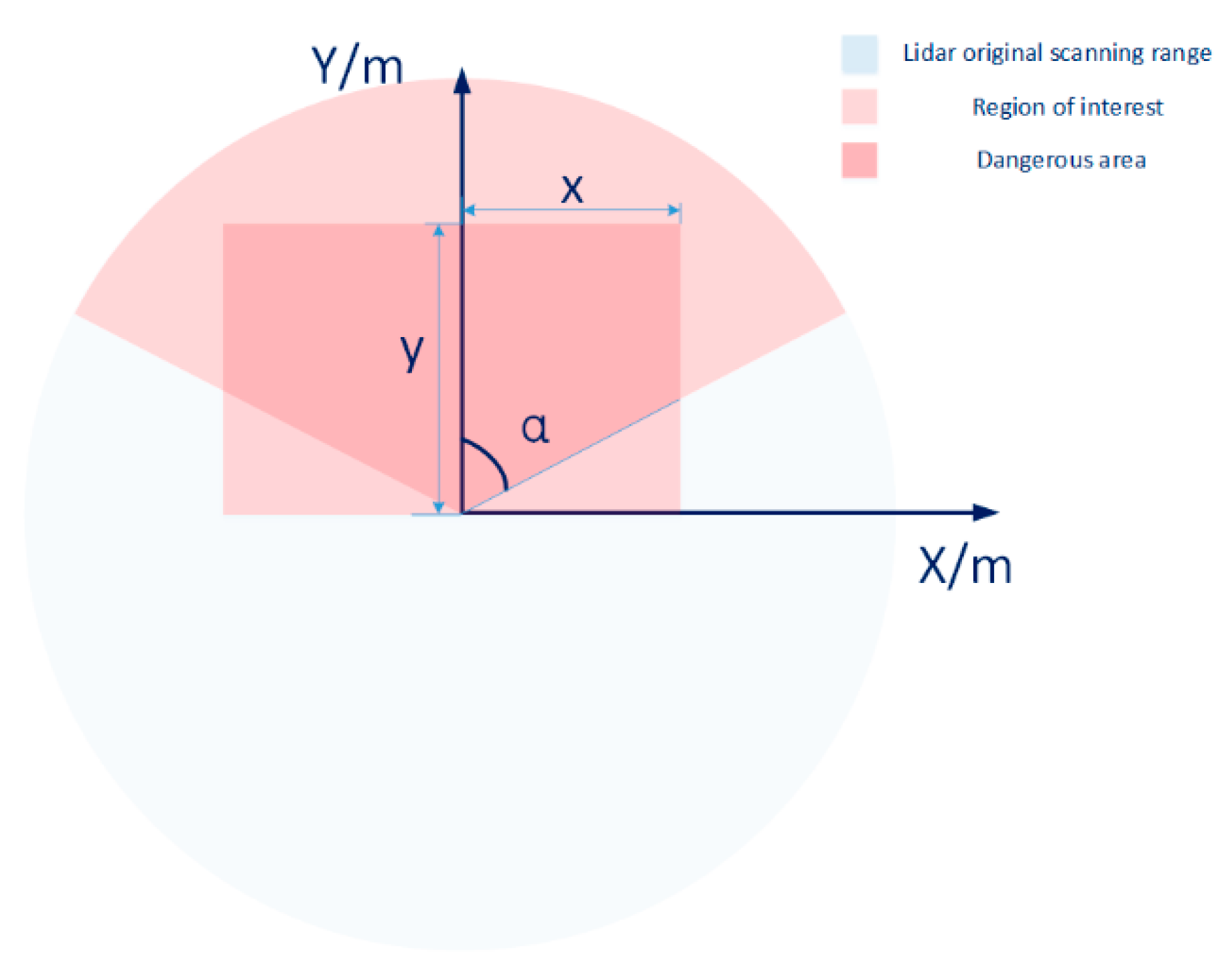
The raw data output by the lidar were in polar coordinates. The angle was α , and the detected distance was d . The position of the 0-degree angle was directly in front of the lidar. The angle increased clockwise to 360 degrees. During pre-processing, first, the angular and distance ranges of the region of interest were determined according to the installation location and the application scenario. The left boundary angle of the ROI was α L , and the right boundary angle was α R . The data in the region of interest were extracted and converted into a rectangular coordinate system. A schematic diagram of the region of interest is shown in Figure 2. The conversion formula is shown in Formula 1.
{ x = d sin α y = d cos α           α [ α L , α R ]

2.2.2. Filtering

Due to the special environment of agricultural machinery operation, some ambient light or dust interfered with the test data during the sensing process. This noise was an impulse noise. It was very similar to the salt and pepper noise in the field of image processing. This noise could be caused by sharp and sudden disturbances in the signal. An effective noise reduction method for this type of noise is a median filter or a morphological filter. To eliminate the influence of these noise points on obstacle detection, we performed median filtering on the collected data.
Median filtering is a nonlinear signal processing method to eliminate outlier noise. For each data point to be processed, the data in the left and right neighborhoods are selected for sorting according to the selected window length, and the value of the middle size is selected as the value of this point after filtering. Compared with the mean filter, the median filter could filter out the salt and pepper noise caused by the dust in the lidar perception. The window size of the median filter selected in this study was 5. The bubble sort method, which is a comparison sort, is named for the way the larger elements “bubble” up to the top of the list [20]. It was used to determine the value of the middle size in the window. An algorithm diagram of median filtering is shown in Figure 3.

2.2.3. DBSCAN Clustering

Obstacles in the field include static obstacles and dynamic obstacles, and multiple obstacles may appear in the area of interest at the same time. In order to cope with such complex perception scenarios, multiple obstacles need to be distinguished to facilitate subsequent algorithms to calculate the size information and motion state information of each obstacle.
This study used a density-based spatial clustering of applications with noise (DBSCAN) method to distinguish multiple obstacles. The algorithm divided the points with sufficient density into clusters and found clusters of arbitrary shapes in the noisy data sequence. When applying this algorithm, we first determined the minimum number of points ( N min _ p o i n t s ) of each cluster and the maximum distance threshold ( ε ) between two adjacent points during clustering according to the sizes of common obstacles in the field and the resolution of the lidar. Each cluster was the largest collection of densely connected points. When clustering, an unclustered point was randomly selected as a seed point for each frame of data, and the distance ( d n ) between the seed point and the point to be clustered was calculated.
d n = ( x s e e d x c u r ) 2 + ( y s e e d y c u r ) 2 2
In the formula, x s e e d and y s e e d are the abscissa and the ordinate of the seed point, respectively, and x c u r and y c u r are the abscissa and ordinate of the current point, respectively.
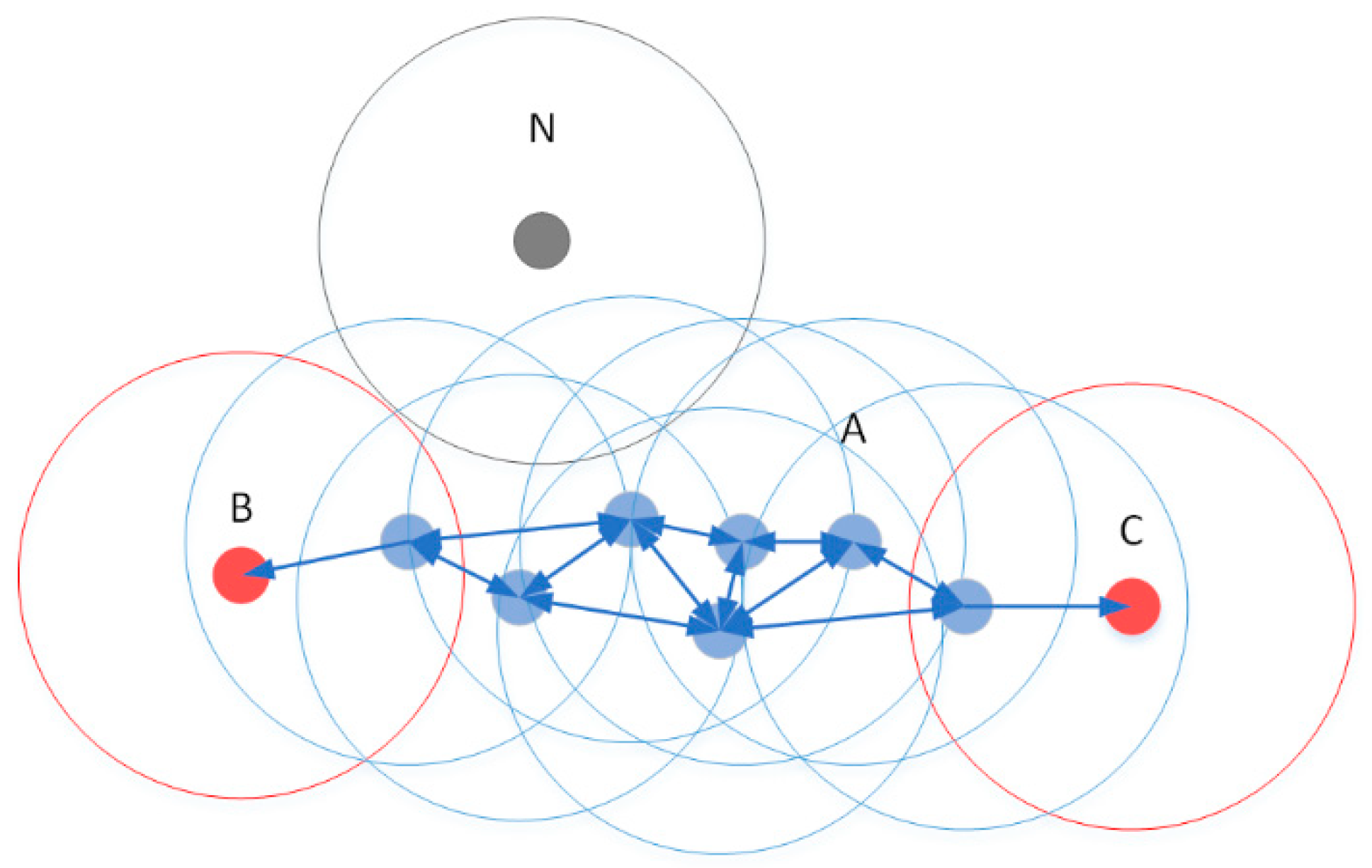
ε was the distance threshold of clustering. If d n ε , the current point was the direct density reachable point of the seed point, and the density reachable point of this point was calculated in turn. The set of these points was a cluster. Each point of the cluster was the center, and the cluster was extended with ε as the radius. If there were other unclustered points within this range, the points were expanded as points within the cluster. They expanded sequentially until the number of points in the cluster no longer expanded. If the number of points in the cluster was greater than N min _ p o i n t s , the cluster became an obstacle. Subsequently, the same calculation was performed on the other unclustered points in the region of interest until the number of clusters no longer increased. Then, the cluster was divided into multiple obstacles. The number of clusters is considered the number of obstacles. Each obstacle cluster had an ID value. A simple schematic diagram of the clustering process is shown in the figure below. In Figure 4, A is the core point, B and C are the boundary points of the cluster, and N is the outlier point of the cluster.

2.2.4. Obstacle Information Calculation

After the above processing, each frame of data was clustered into one or more obstacles, and the number of obstacles was obtained from the number of clusters. Through the analysis of each obstacle cluster, the real-time width information of the obstacle could be obtained, and by analyzing the obstacle clusters between the two frames of data, the motion state information of the obstacles, such as the relative speed and time to collision (TTC), could be obtained.
The maximum and minimum values of the abscissa of each obstacle cluster point were calculated to obtain the horizontal boundary [ x l ,   x r ] of the obstacle. Then, the real-time width ( W ) of the obstacle was
W = | x r x l |
To obtain the motion state information of the obstacle, it was necessary to perform differential processing on the obstacle data in the two frames of data. In order to cope with a scene with multiple obstacles, it was first necessary to perform interframe matching on the obstacles between the two frames of data to ensure that the obstacle in the current frame and the obstacle in the previous frame represented the same obstacle. In this study, two criteria were used for interframe matching; one was the width of the obstacle, and the other was the point of the obstacle. For two obstacles to be the same obstacle in two frames of data, first, the difference between the widths of the two obstacles must be less than the threshold ( ω ), and second, in the current frame, the abscissa value ( x p ) of a certain point in the obstacle cluster is within the range of the abscissa of an obstacle in the previous frame:
| W c u r W p r e | ω
x l x p x r
Each obstacle cluster in the previous frame and the current frame were traversed in turn, and the ID-matching pair of obstacles between the two frames was obtained. After obtaining the obstacle matching between the two frames, the relative speed and collision time of the lidar and the obstacle could be obtained by combining the distance difference of the obstacle between the two frames and the frame rate.
When calculating the distance between an obstacle and the lidar, if the intermediate point of the obstacle was directly calculated, there could have been deviations due to the appearance of individual deviation points in the data. In this study, the 6σ method was used to eliminate the deviation in the data, and the distance between the obstacle and the lidar was obtained using the average value of the qualified points. The 6σ method originated in quality management and is a statistical quality control method. In this study, it was used to deal with the longitudinal distance of lidar scanning obstacles. The ordinates of the cluster points of a certain obstacle in the current frame were { y 1 ,   y 2 y n } . Their average was calculated as y ¯ , and the standard deviation was calculated as σ y . The ordinates of the cluster points of the obstacle in the previous frame were { y 1 ,   y 2 y n } . Their average value was calculated as y ¯ , and their standard deviation was calculated as σ y . The ordinate of any point of the obstacle in the current frame was y i , and all ordinate points that satisfied the following formula were found:
| y i y ¯ | < 3 σ y
The average value of all ordinates that met this requirement was calculated as the longitudinal distance ( d c u r ) of the obstacle from the lidar in the current frame. The ordinate of any point of the obstacle in the previous frame was y i , and the same method was used to calculate all ordinates in the previous frame that satisfied the following formula:
| y i y ¯ | < 3 σ y
The same method was used to calculate the average value of all ordinates that met this requirement as the longitudinal distance ( d p r e ) from the obstacle to the lidar in the previous frame. According to the distance change and the time interval between the two frames, the relative movement speed ( v ) was obtained.
v = d p r e d c u r Δ t = d p r e d c u r 1 / F P S
In the formula, Δ t is the time interval between the two frames of data and F P S is the frame rate of the lidar. According to the current distance between the obstacle and the lidar and the above-mentioned relative movement speed, the remaining time ( t ) before the obstacle would collide with the lidar could be obtained as:
t = d c u r v = d c u r ( d p r e d c u r ) F P S
Using the same method, the time for each remaining obstacle to collide with the lidar was calculated to provide parameter support for the subsequent development of the pre-collision system.

2.3. Emergency Braking Strategy and Software Development

2.3.1. Emergency Braking Strategy

After the above processing, parameters such as the number of obstacles, the width of each obstacle, the relative movement speed of the agricultural machine, and the time until collision with the agricultural machine were obtained. When these parameters were applied to the agricultural machinery pre-collision system, two main judgment strategies were used to decide whether to make an emergency stop: 1. A TTC safety threshold ( T ε ) was set according to the speed of the vehicle and the movement speed of common obstacles in the work area. If there was any obstacle whose TTC is less than T ε , the vehicle was stopped. 2. A dangerous area around the vehicle was set according to the operation type and the application scenario of the agricultural machinery. In this research, the area was symmetrical about the Y axis directly in front of the lidar, and the area could be set by the X and Y values. For each frame of obstacle data processed, it was judged whether the point closest to the lidar was in the dangerous area by setting the X and Y values. If there was any obstacle in the area, the vehicle stopped. The division of areas is shown in Figure 5.

2.3.2. Software Development

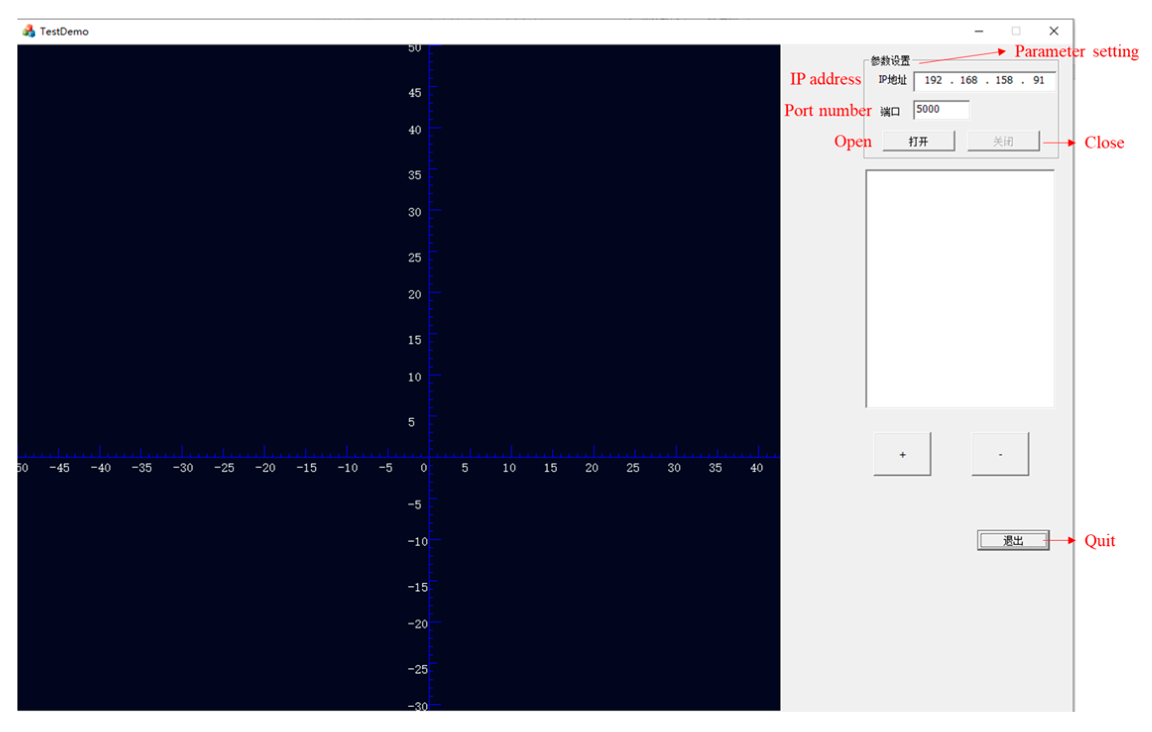
To apply the algorithm to the actual agricultural machinery operation, we developed the program of the algorithm. The real-time pre-collision system used C++ programming and combines the MFC library [21] to compile the lidar communication and real-time detection display interface. The software could fill in the IP of the lidar so that the processor’s network and the lidar were in the same network segment to establish communication. When the system was running, the black display area of the display interface would highlight the point of the obstacle. Moreover, if an obstacle was detected through algorithm processing that threatened driving safety and required a stop, the system would issue a stop command, and at the same time a prompt sentence would be output in the text box on the right side of the interface to allow the debugger or user to observe and confirm. A data processing flow diagram of the software is shown in Figure 6, and the software interface is shown in Figure 7.

2.4. Design of a Harvester Pre-Collision System

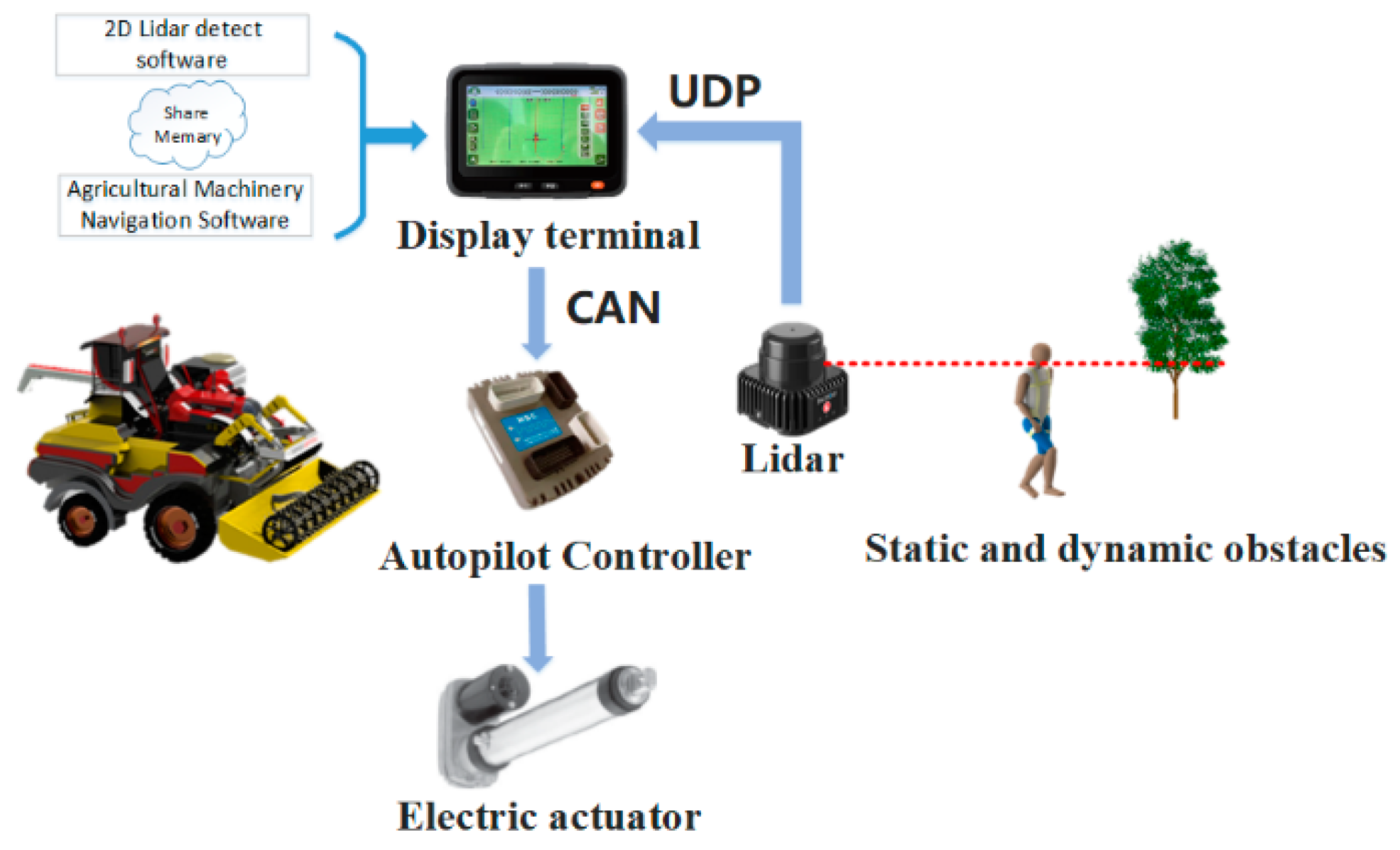
To verify the effectiveness of the algorithm and apply it to actual agricultural machinery operations, we designed a harvester pre-collision system. The system directed the harvester to stop when encountering dangerous obstacles based on the obstacle information detected by the lidar. The system included a lidar, a display terminal, an automatic navigation controller, and actuators. A schematic diagram of the hardware design of the system is shown in Figure 8.
The lidar sent the data to the display terminal through the network interface using the UDP protocol. The terminal had 2 G of memory, a 32 G solid-state hard drive, and a Windows 10 operating system. The agricultural machinery pre-collision system software developed in C++ ran on the terminal, and the software could use the algorithm mentioned above to process the lidar data. At the same time, to achieve an unmanned effect during the test, the system was integrated with the agricultural machinery automatic driving system, and the automatic driving software was also running on the terminal. The result, processed by the pre-collision system, was sent to the autonomous driving program on the terminal through shared memory. The terminal sent the instruction of whether to stop to the automatic driving controller through the CAN bus. Through the modification of the harvester, an electric push rod was used as an actuator to replace the gear in the cab to control the forward motion, stopping, and reversing of the vehicle body. The controller controlled the extension and contraction of the electric actuator through the IO port to control the driving and parking of the vehicle body.
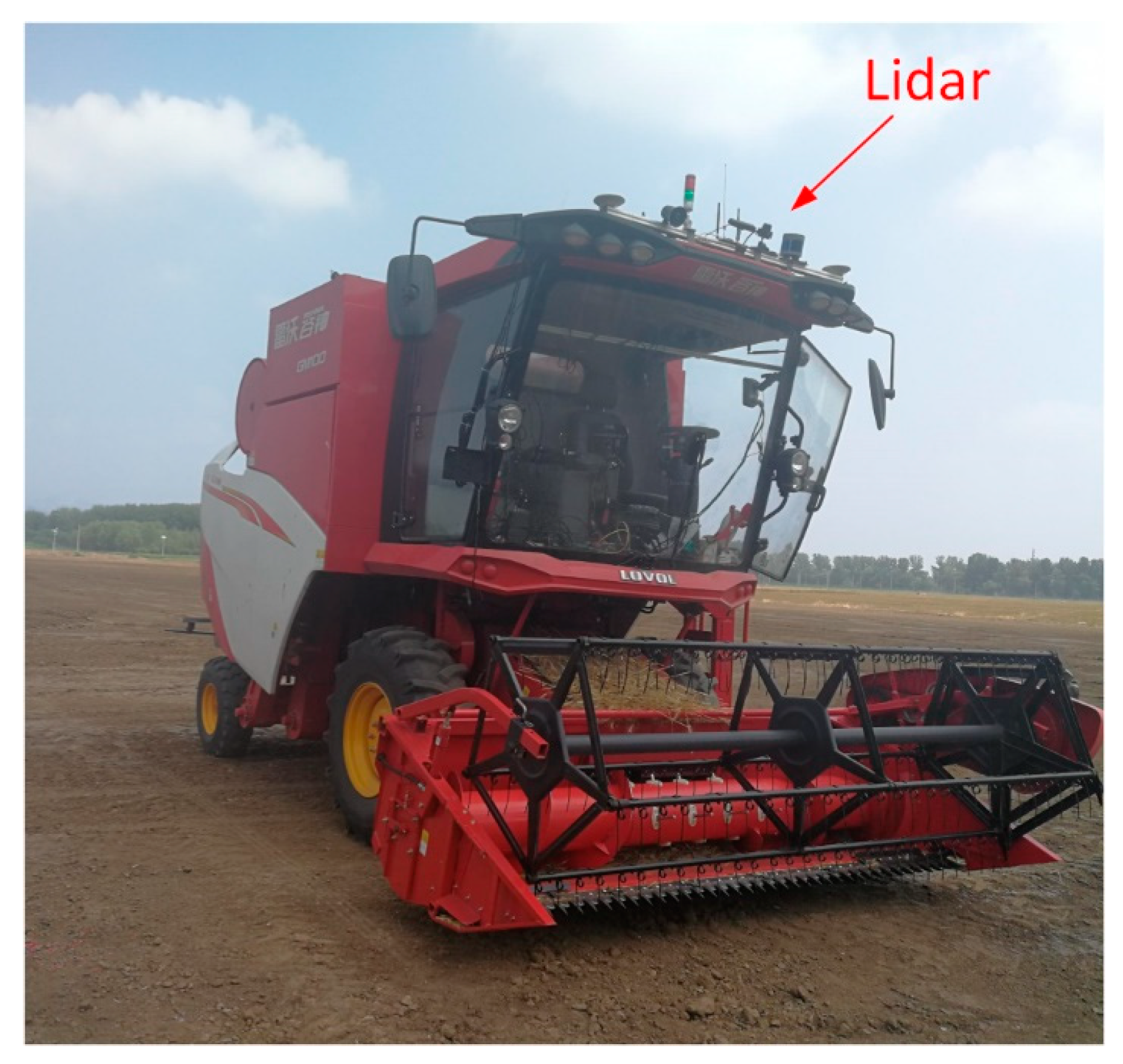
The harvester used in this study was a Lovol Gushen GM-100 (Weifang City, Shandong Province, China)wheat combine harvester. Due to the particularity of the harvester, when selecting the installation position of the lidar, to avoid the false recognition of obstacles caused by lifting the header and reel, the lidar was installed above the cab in this study. Moreover, the height of the harvester was 3.2 m. To detect low obstacles while ensuring the detection range of the lidar and reducing blind spots, the scanning surface of the lidar was tilted down by 20°. During installation, the 0° direction of the lidar scan was the same as the front of the harvester, which was the positive direction of the Y axis, and the 90° direction was the positive direction of the X axis of the coordinate system. Lidar installation pictures are shown in Figure 9. To facilitate subsequent tests, the pre-collision system was integrated with the agricultural unmanned driving system. During the test, the display terminal and controller were installed in the cab to facilitate debugging and the viewing of obstacles. An installation picture is shown in Figure 10.
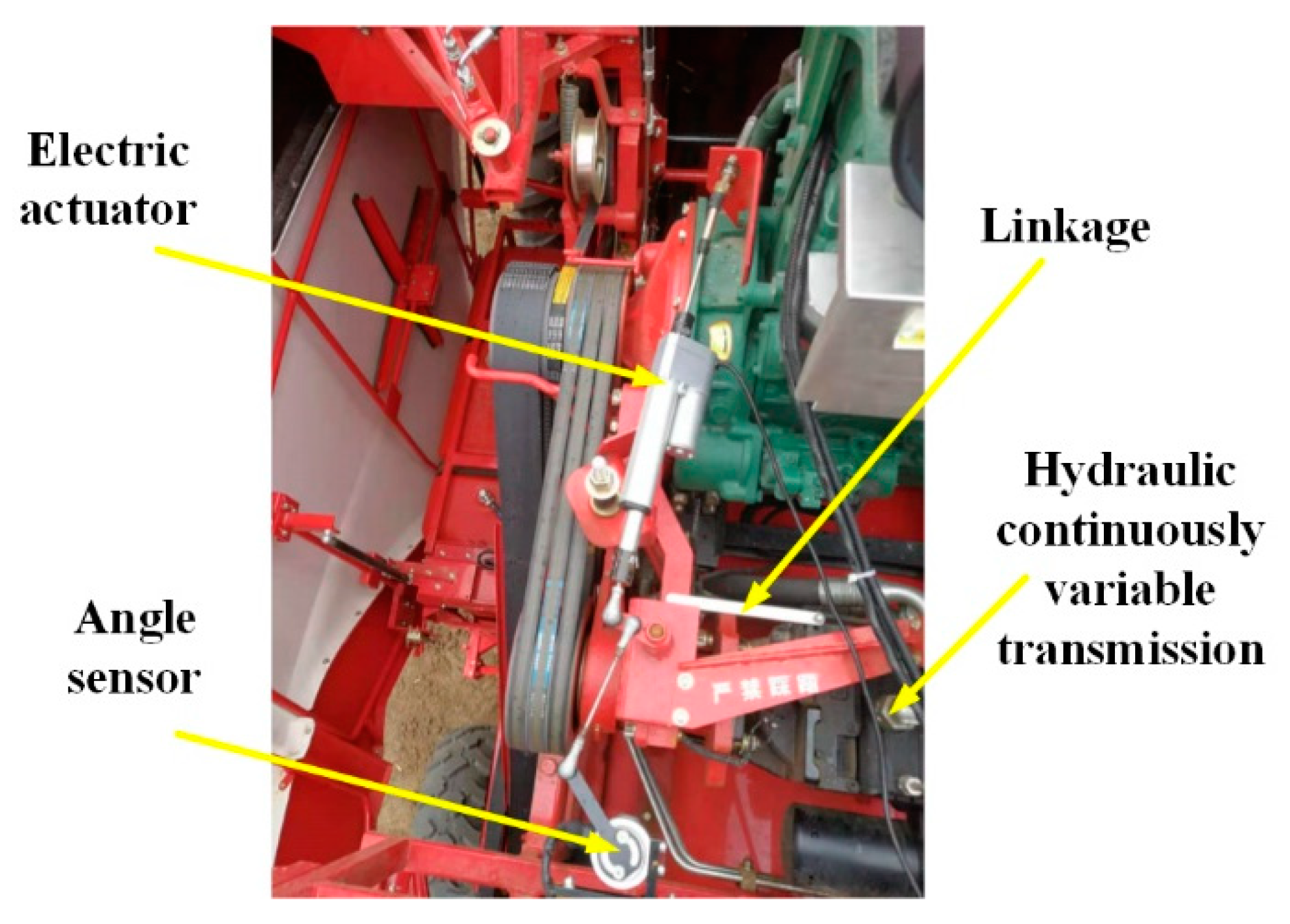
In order to allow the system to automatically stop when it detected an emergency, we carried out an electronic control modification to the harvester. An electric actuator replaced the function of shifting in the cab to realize a program-controlled stop. The electric actuator was connected with the hydraulic continuously variable transmission on the vehicle body through a linkage mechanism. An installation picture is shown in Figure 11. The body stopped when the electric push rod was in the neutral position. The contraction and extension of the electric push rod, respectively, controlled the forward and backward movement of the body. The position of the push rod was fed back to the controller through an angle sensor. The controller controlled the expansion and contraction of the push rod through the IO port to control the stopping and movement of the body.

2.5. Experiment

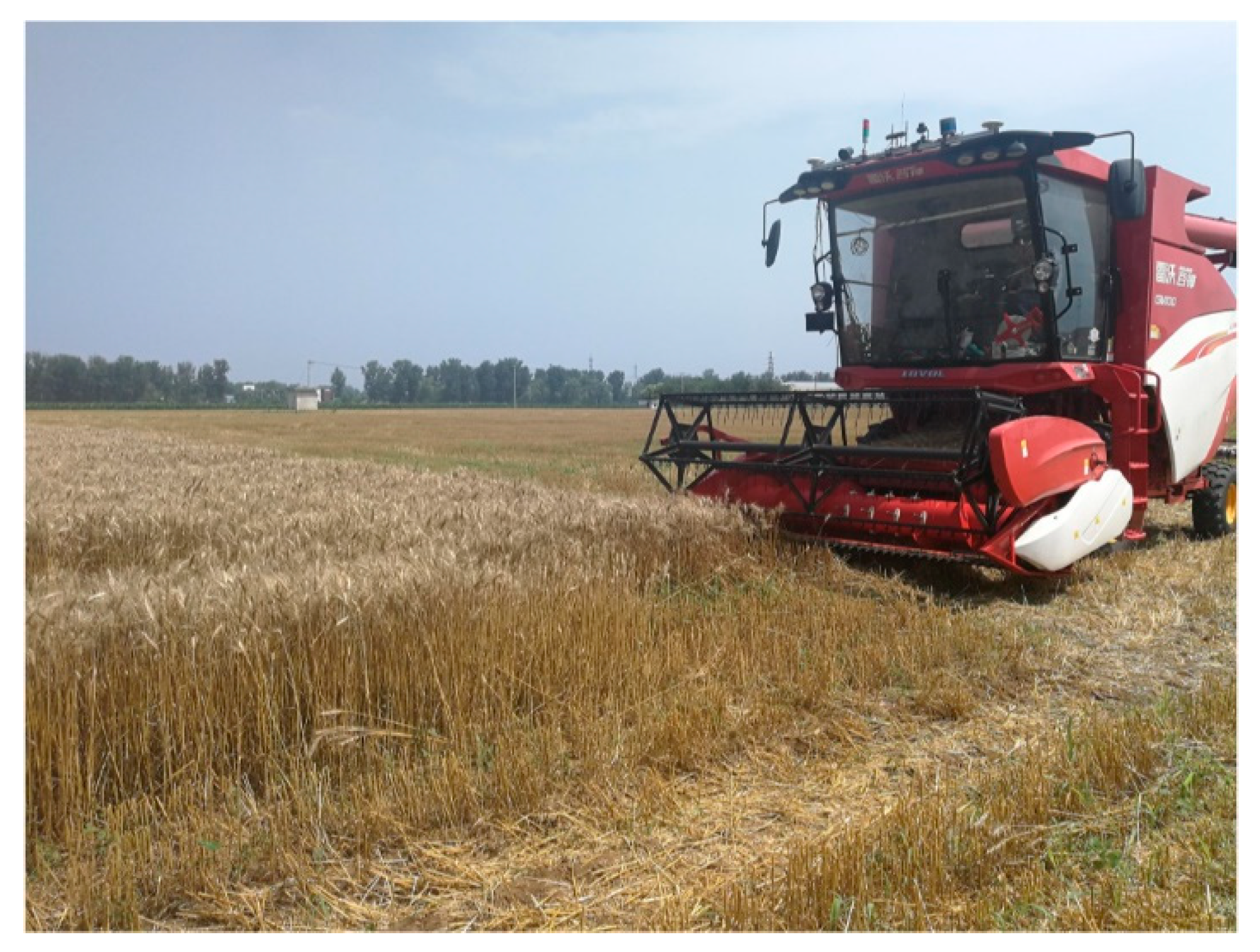
In order to test the detection error of the algorithm and evaluate the effectiveness of the system, we applied a system to the harvester and carried out field trials at the Beijing Xiaotangshan National Experiment Station for Precision Agriculture in June 2021. During the test, two main experiments were carried out; one was the multi-obstacle detection test, and the other was the pre-collision stopping vehicle test. The lidar was installed at the transverse center in front of the top of the harvester cab, with a downward tilt of about 17 degrees and an installation height of about 3.2 m. The lidar was fixed on the harvester with a bracket to ensure its relative position remained unchanged to avoid a change in position affecting the recognition results. Assuming that the height of wheat is 1 m, in order to avoid detecting wheat by mistake when detecting obstacles, the wheat part was not included when setting the region of interest. A schematic diagram is shown in Figure 12. The multi-obstacle detection test was carried out under an actual harvest scenario. During the test, several people were arranged to walk irregularly in front of the harvester to verify its detection effect. The pre-collision stopping vehicle test was a dynamic test. During the test, the harvester was driven into the wheat field for automatic driving operation, and the normal driving speed was 5 km/h. At the same time, people walked in front of the harvester as an obstacle to test whether the system detected and stopped effectively.
In the experiment, the angular boundary range of the region of interest was set to [−70°, 70°]. Moreover, because of the harvester’s particularity, the lidar’s installation had an inclination angle. In order to avoid the false detection of wheat, according to the inclination angle and the height of the wheat (the average height in this experiment was 70 cm), the distance range was set to 7.3 m. The sliding window size of the median filter was 5. The minimum number of clustering points was 4, and the clustering distance threshold was 0.75 m. The TTC safety threshold was 30 s. According to the width of the harvester, the extended length of the header, and the speed of the vehicle, the x range of the dangerous area was set to [−3, 3], and the range of y was [0, 4]. A test picture is shown in Figure 13.

3. Results and Discussion

3.1. Multi-Obstacle Detection Results

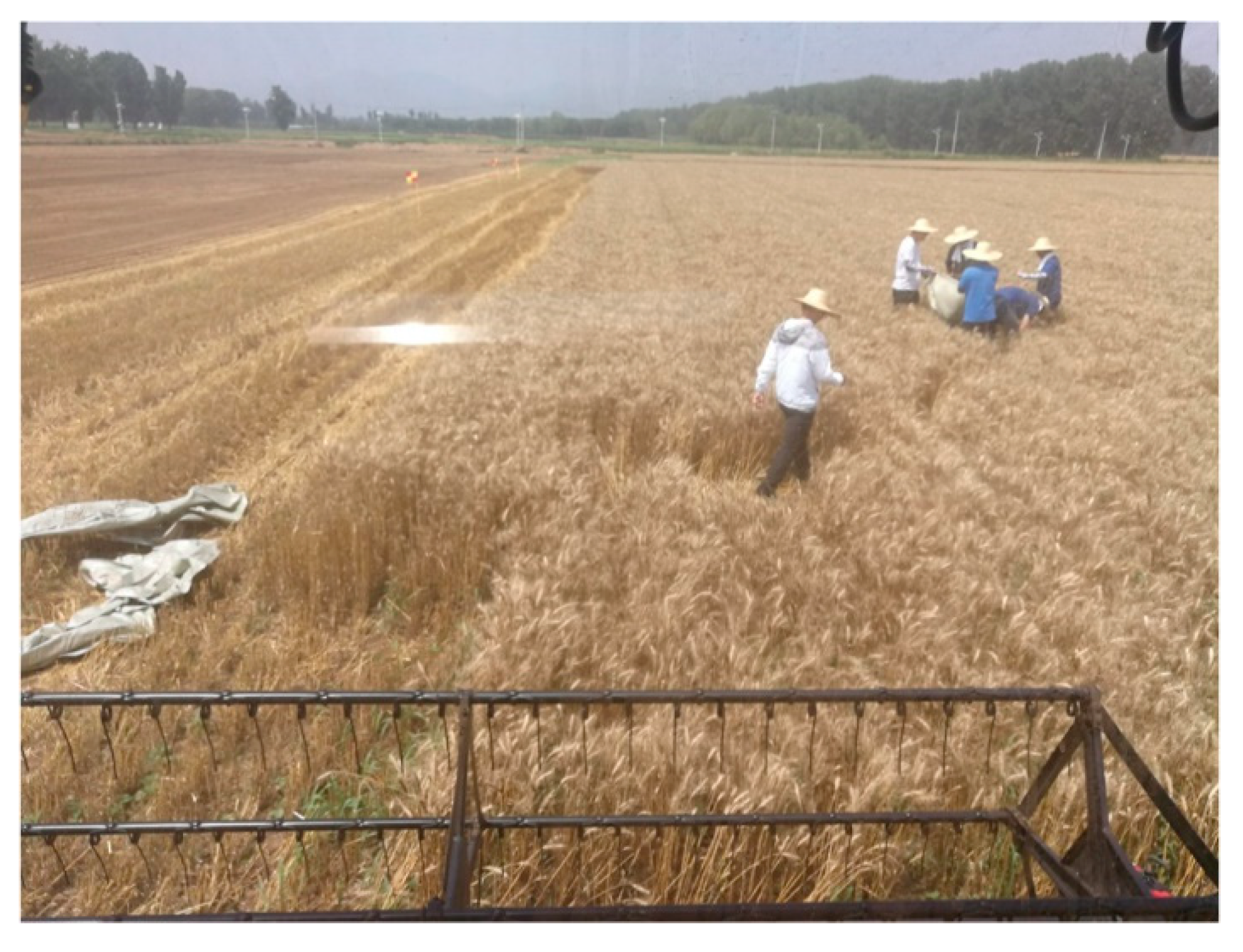
In order to test the detection effect of the algorithm on multiple obstacles, during the test multiple people in the wheat field were tested as obstacles. The heights of the people in the experiment were 1.75–1.82 m. A test picture is shown in Figure 14. The lidar data were processed according to the above algorithm steps, and the data of each step were recorded for analysis. Each processing step is shown in Figure 15.
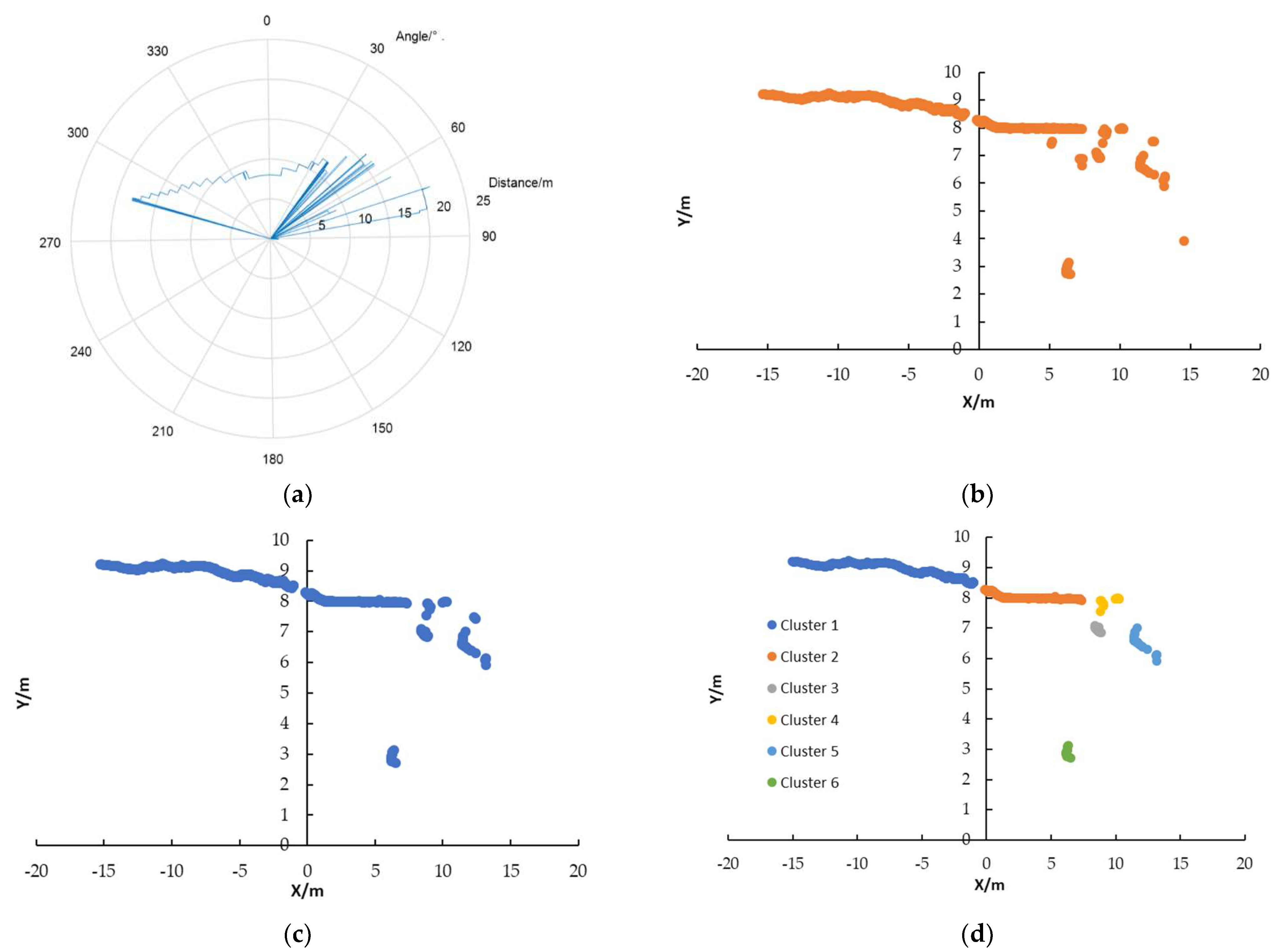
Figure 15 shows the processing effect of the algorithm at each step. Figure 15a is the original lidar data in the polar coordinate system. It can be seen in the figure that due to the installation position and angle of the lidar and because its left and right sides were blocked, most of the returned lidar data were in the front. The data from the region of interest that were extracted and converted to the rectangular coordinate system are shown in Figure 15b. It can be seen in the figure that there was some reduction in the data after the region of interest was extracted, and there were some outliers on the right side of the figure. After filtering, the partial separation group points disappeared, as shown in Figure 15c. The result of clustering the processed data is shown in Figure 15d. There are six clusters in the figure. Compared with the previous figure, two points are not shown in the figure because they did not meet the clustering conditions. Each different cluster is represented by a different color.
Figure 15 was compared with Figure 14 to analyze the obstacle information. Cluster 1 in blue was the harvested ground, with few ups and downs. Cluster 2 in orange was an unharvested wheat field with a relatively stable height. The gap between the two clusters was the harvest boundary. Since the forward center of the installed lidar was close to the left side of the vehicle body and the harvester was closer to the harvesting boundary on the left side, the lateral center of the collected lidar data was near the harvesting boundary. Because the lidar had an installation inclination angle, combined with the wheat’s height and the stubble’s height after harvest, the longitudinal distance of the detected wheat and the ground was also consistent with the actual situation. Cluster 3 in gray, cluster 4 in yellow, and cluster 5 in light blue in the upper right of the graph correspond to the four people in the front right and far away from the harvester in the experimental graph. Since the lidar installation had a certain scanning angle and these people were relatively close, two people were clustered as one obstacle during the clustering. However, it did not affect the overall pre-collision effect. Cluster 6 in green at the bottom right of the graph corresponds to the white-clothed person near the harvester in the experimental picture. It can be seen from the experiment that the application of this algorithm can realize low-cost two-dimensional lidar harvester multi-obstacle detection.
A total of 223 frames of data were collected and clustered during the multi-obstacle detection, of which 212 frames were correctly clustered. The accuracy rate of the multi-obstacle detection was 95.06%.

3.2. Pre-Collision Results

In order to test whether the pre-collision system could stop autonomously after detecting dangerous obstacles, we conducted a test. In order to test the effect of the pre-crash system, experiments were carried out in this research. During the test, humans acted as obstacles within the detection range of the lidar to test whether the system could stop autonomously after detecting dangerous obstacles. During the test, the number of obstacles that occurred in front of the harvester and the number of vehicle stops were recorded. The test results’ precision rate and recall rate were calculated to analyze the system’s abnormal situation.
P = T P T P + F P
R = T P T P + F N
where P is the precision rate and R is the recall rate; T P is the number of times an obstacles occurred and the vehicle stopped correctly; F P is the number of times an obstacles occurred and the vehicle did not stop; and F N is the number of times the vehicle stopped without obstacles. The harmonic mean value (F) of the precision rate and recall rate is
F = ( α 2 + 1 ) × P × R α 2 ( P + R )
In the formula, α is the value of the harmonic parameter. Under normal circumstances, the value of α is 1. In this case, F is
F 1 = 2 × P × R P + R
Five groups of experiments were conducted in this study. Each group included 4–6 anti-collision tests. The number of trials and the number of successful trials in each group were recorded. The recorded data analysis is shown in Table 2.
It can be seen in Table 2 that in the five groups of experiments that were carried out, tests 1, 2, and 5 could all stop correctly. However, in test groups 3 and 4, the number of vehicle stops was less than the number of obstacles that occurred; that is, there was a situation where an obstacle appeared, but the vehicle did not stop. This led to a drop in the recall rate. The reason may be that the obstacle was not within the effective detection range of the lidar, causing the failure to stop the vehicle. Alternatively, the obstacle was not in the danger zone, and the time to collision had not reached the set threshold, so the vehicle did not stop. In this situation, the harmonic mean values of the third and fourth groups were 88.89% and 90.91%, respectively. The average precision rate was 92.67%. The average harmonic mean value was 95.96%.

4. Conclusions

This research used low-cost two-dimensional lidar to detect obstacles in farmland. An algorithm for identifying multiple obstacles and calculating each obstacle’s size and movement status was proposed. The algorithm performed pre-processing to delineate the region of interest, perform coordinate conversion, and filter the data. Then, it used the density-based clustering method to obtain the number and width of each obstacle. Finally, the relative motion speed and the time to the collision for each obstacle and the vehicle body were obtained based on the interframe difference algorithm. This algorithm was used to realize the software development of agricultural machinery pre-collision systems, using Windows as the system platform and C++ as the programming language. Multi-obstacle tests and pre-collision tests were carried out on the system. The test results showed that the system could effectively detect multiple obstacles. The accuracy rate of multi-obstacle detection was 95.06%. The accuracy rate of stopping when dangerous obstacles were detected was 92.67%. The harmonized average of the accuracy and recall rates was 95.96%. This research provides a foundation for the safe autonomous driving of agricultural machinery. In the future, more complex and efficient obstacle circumvention strategies can be studied based on the number, width, speed, and other parameters of the detected obstacles.

Author Contributions

Conceptualization, Y.S., Z.S. and Z.M.; methodology, Y.S., Z.S. and Z.M.; software, H.W.; validation, W.Q.; formal analysis, Q.W.; investigation, H.L.; resources, Z.S. and Z.M.; data curation, Y.Y.; writing—original draft preparation, Y.S.; writing—review and editing, Y.S.; visualization, H.W.; supervision, Z.S.; project administration, Z.M.; funding acquisition, Z.S. and Z.M. All authors have read and agreed to the published version of the manuscript.

Funding

This research was funded by the National Key Research and Development Program of China (grant number: 2022YFD2001603) and the Jiangsu Provincial Agricultural Science and Technology Independent Innovation Fund Project (grant number: CX (20)1007).

Data Availability Statement

All data are presented in this article in the form of figures or tables.

Acknowledgments

We would like to thank the “College of Engineering, China Agricultural University”, “Research Center of Intelligent Equipment, Beijing Academy of Agriculture and Forestry Sciences”, and “AgChip Science and Technology (Beijing) Co., Ltd.”.

Conflicts of Interest

The authors declare no conflict of interest.

References

  1. Zhang, S.; Tian, X.; Wang, S. Impact of aging agricultural labor on mechanization and technical efficiency in wheat production: A perspective analysis based on landforms. J. China Agric. Univ. 2018, 23, 174–182. [Google Scholar] [CrossRef]
  2. Zhang, M.; Ji, Y.; Li, S.; Cao, R.; Xu, H.; Zhang, Z. Research progress of agricultural machinery navigation technology. Trans. Chin. Soc. Agric. Mach. 2020, 51, 1–18. [Google Scholar] [CrossRef]
  3. Rahman, M.M.; Ishii, K.; Noguchi, N. Optimum harvesting area of convex and concave polygon field for path planning of robot combine harvester. Intel. Serv. Robot. 2019, 12, 167–179. [Google Scholar] [CrossRef] [Green Version]
  4. He, Y.; Jiang, H.; Fang, H.; Wang, Y.; Liu, Y. Research progress of intelligent obstacle detection methods of vehicles and their application on agriculture. Trans. Chin. Soc. Agric. Eng. 2018, 34, 21–32. [Google Scholar] [CrossRef]
  5. Dvorak, J.S.; Stone, M.L.; Self, K.P. Object detection for agricultural and construction environments using an ultrasonic sensor. J. Agric. Saf. Health 2016, 22, 107–119. [Google Scholar] [CrossRef] [PubMed]
  6. Wei, J.; Han, S.; Reid, J.F.; Han, S. Obstacle detection using stereo vision to enhance safety of autonomous machines. Trans. ASABE 2005, 48, 2389–2397. [Google Scholar] [CrossRef]
  7. Zhang, L.; Wang, S.; Chen, B.; Liu, Z. Detection of obstacles in farmland based on binocular vision. J. China Agric. Univ. 2007, 12, 70–74. [Google Scholar]
  8. Ding, Y.; Wang, S.; Chen, H. Obstacle detection in the working area of agricultural vehicle based on machine vision. Trans. Chin. Soc. Agric. Mach. 2009, 40 (Suppl. 1), 23–27. [Google Scholar]
  9. Yin, X.; Noguchi, N.; Ishi, K. Development of an obstacle avoidance system for a field robot using a 3D camera. Eng. Agric. Environ. Food 2013, 6, 41–47. [Google Scholar] [CrossRef]
  10. Brenneke, C.; Wagner, B. A Scan Based Navigation System for Autonomous Operation of Mobile Robots in Man-Made Environments. In Proceedings of the International Conference of Systems Engineering, Institute for System Engineering, Hannover, Germany, 1 January 2003. [Google Scholar]
  11. Jiménez, F.; Naranjo, J.E. Improving the obstacle detection and identification algorithms of a laser scanner-based collision avoidance system. Transp. Res. Part C Emerg. Technol. 2011, 19, 658–672. [Google Scholar] [CrossRef]
  12. Asvadi, A.; Premebida, C.; Peixoto, P.; Nunes, U. 3D Lidar-based static and moving obstacle detection in driving environments. Robot. Auton. Syst. 2016, 83, 299–311. [Google Scholar] [CrossRef]
  13. Zeng, L.; Feng, J.; He, L. Semantic segmentation of sparse 3D point cloud based on geometrical features for trellis-structured apple orchard. Biosyst. Eng. 2020, 196, 46–55. [Google Scholar] [CrossRef]
  14. Doerr, Z.; Mohsenimanesh, A.; Lagu, C.; Mclaughlin, N. Application of the LIDAR technology for obstacle detection during the operation of agricultural vehicles. Can. Biosyst. Eng. Le Genie Des Biosyst. Au Can. 2013, 55, 2.9–2.16. [Google Scholar] [CrossRef] [Green Version]
  15. Takahashi, M.; Kobayashi, K.; Watanabe, K.; Kinoshita, T. Development of prediction based emergency obstacle avoidance module by using LIDAR for mobile robot. IEEE Int. Symp. Soft Comput. Intell. Syst. 2015, 2014, 561–564. [Google Scholar] [CrossRef]
  16. Peng, Y.; Qu, D.; Zhong, Y.; Xie, S.; Luo, J.; Gu, J. The Obstacle Detection and Obstacle Avoidance Algorithm Based on 2-D Lidar. In Proceedings of the IEEE International Conference on Information and Automation, Lijiang, China, 10 August 2015. [Google Scholar] [CrossRef]
  17. Reina, G.; Milella, A.; Rouveure, R.; Nielsen, M.; Worst, R.; Blas, M.R. Ambient awareness for agricultural robotic vehicles. Biosyst. Eng. 2016, 146, 114–132. [Google Scholar] [CrossRef]
  18. Kragh, M.; Underwood, J. Multi-Modal Obstacle Detection in Unstructured Environments with Conditional Random Fields. J. Field Robot. 2017, 37, 53–72. [Google Scholar] [CrossRef] [Green Version]
  19. Xue, J.; Fan, B.; Yan, J.; Dong, S. Trunk detection based on laser radar and vision data fusion. Int. J. Agric. Biol. Eng. 2018, 11, 20–26. [Google Scholar] [CrossRef]
  20. Cormen, T.H.; Leiserson, C.E.; Rivest, R.L.; Stein, C. Introduction to Algorithms, 2nd ed.; MIT Press: Cambridge, MA, USA; McGraw-Hill: New York, NY, USA, 2001; Problem 2–2; p. 40. ISBN 0-262-03293-7. [Google Scholar]
  21. Visual Studio 2019 Release Notes. Available online: Msdn.microsoft.com (accessed on 24 July 2019).
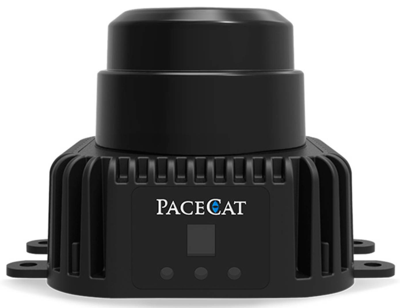
Figure 1. The lidar used in this research.
Agronomy 13 00388 g001
Figure 2. Region of interest and coordinate system.
Agronomy 13 00388 g002
Figure 3. Schematic diagram of the median filter.
Agronomy 13 00388 g003
Figure 4. Schematic diagram of the DBSCAN algorithm.
Agronomy 13 00388 g004
Figure 5. Data processing area comparison.
Agronomy 13 00388 g005
Figure 6. Schematic diagram of the data processing flow.
Agronomy 13 00388 g006
Figure 7. The software interface.
Agronomy 13 00388 g007
Figure 8. Design schematic diagram of the harvester pre-collision system.
Agronomy 13 00388 g008
Figure 9. Lidar installation.
Agronomy 13 00388 g009
Figure 10. Display terminal and controller pictures: (a) display terminal; (b) controller.
Agronomy 13 00388 g010
Figure 11. Electric linear actuator installation.
Agronomy 13 00388 g011
Figure 12. The installation position and obstacle detection of the lidar on the harvester.
Agronomy 13 00388 g012
Figure 13. The experiment.
Agronomy 13 00388 g013
Figure 14. Multi-obstacle detection.
Agronomy 13 00388 g014
Figure 15. Data processing diagram of each step: (a) raw data in a polar coordinate system; (b) data in the ROI in a Cartesian coordinate system; (c) filtered data; (d) clustered data.
Agronomy 13 00388 g015
Table 1. Main parameters of the lidar.
ParametersValue
Measuring range (m)0.1–40
Ranging accuracy (cm)±3
Field of view (°)360
Angle resolution (°)0.09–0.27
Rotating speed (r/min)300–900
Table 2. Analysis of pre-collision system test.
Test GroupNumber of FramesThe Number of Obstacles That OccurredThe Number of Vehicle StopsPrecision RateRecall RateHarmonic Mean Value
179155100%100%100%
284944100%100%100%
36105480%100%88.89%
412746583.33%100%90.91%
534155100%100%100%
Disclaimer/Publisher’s Note: The statements, opinions and data contained in all publications are solely those of the individual author(s) and contributor(s) and not of MDPI and/or the editor(s). MDPI and/or the editor(s) disclaim responsibility for any injury to people or property resulting from any ideas, methods, instructions or products referred to in the content.