The Dynamic Response of Runoff to Human Activities and Climate Change Based on a Combined Hierarchical Structure Hydrological Model and Vector Autoregressive Model

Abstract

Climate change refers to a statistically significant change in the average state of the climate or a climate alteration that lasts for a long period of time. Runoff (R) is as a measure of the interaction between climate change and human activities and plays an important role in the hydrological cycle, as it is directly related to the development of agricultural water management. Therefore, it is a requirement to correctly simulate R and have the ability to separate the impacts due to climate change and human activities. In this paper, five single-type simulation models (Back Propagation Neural Network (BP), Non-Autoregressive (NAR), Radial Basis Function (RBF), Support Vector Machine (SVM) and TOPMODEL Hydrological Model (TOPMODEL)) were adopted to simulate the R to analyze the simulating quality by comparing the evaluation indexes like relative error (RE), relative mean squared error (RMSE) and Nash–Sutcliff Efficiency (NSE) with the combined hierarchical structure hydrological (CHSH) simulation model. In traditional studies, only the relative contribution of the impacts of human activities and climate change on R are considered; however, in this study, the relative contribution of each meteorological factor affecting R is included. To quantitatively analyze the impact of human activities and climate change on R, we used a CHSH simulation model to calculate runoff values for the Lancang River of China for a period of nine years (2005–2013). Our objective was to use this type of model to improve both the accuracy and stability of calculated values of R. For example, the RE, RMSE and NSE of simulated monthly R calculated with the CHSH model were 6.41%, 6.67 × 10⁸ m³ and 0.94, respectively. These values substantiate the improved accuracy and stability of calculated values of R obtained with single-type simulation models (the SVM model, for instance, widely used in runoff simulations, and the RE, RMSE and NSE were 14.1%, 12.19 × 10⁸ m³ and 0.87, respectively). The total contribution of human activities and climate change to R, respectively, accounted for 34% and 66% for the nine-year period based on the CHSH model. Furthermore, we adopted a vector autoregressive (VAR) model to analyze the impacts of the meteorological factors on R. The results from this analysis showed that R has a strong fluctuation response to the changes in precipitation (P) and potential water evaporation (E_p). The contribution rates of E_p, P and air temperature (T_a) to R were 15%, 14% and 2%, respectively. Based on the total climate change contribution, the corresponding contribution rates of E_p, T_a and P in the Lancang River of China were 32%, 30% and 5%, respectively. The values of R calculated with the CHSH model are more accurate and stable compared to values obtained with single-type simulation model. Further, they have the advantage of avoiding drawbacks associated when using a single-type simulation model. Moreover, moving away from the traditional method of separating the impact of meteorological factors on R, the vector autoregressive model proposed in this paper can describe the contribution of different meteorological factors on R in more detail and with precision.

1. Introduction

Faced with the increase in population around the world, agricultural water management, as a controversial issue, is important in the efforts to maintain food security. The interactions and feedbacks between human activities and water cycle dynamics, combined with the evolution of human values in relation to water, are creating what have been considered as emerging “big problems” [1]. As the link in the interaction of human activities and the water cycle, runoff plays an increasingly important role in the balance of the ecological value of water and agricultural water management [2]. It is one of the important water sources for downstream agricultural water, and it plays a significantly important role in downstream agricultural irrigation [3]. Especially, the runoff at the downstream of reservoirs is a kind of stochastic process with uncertainty and variability [4,5]. In order to understand and manage the interactions of humans and water in the river basin management, it is important to quantify the impact of human activities and climate change on runoff based on process modeling and statistical analysis.

Traditional long- and mid-term runoff forecast methods include the time-series analysis method [6], principal component analysis (PCA) method [7] and artificial neural network (ANN) [8], while new methods are mainly deep learning [9], grey system analysis [10], wavelet [11] and support vector machines (SVM) [12]. However, both traditional and new methods have some advantages and disadvantages [13]. For example, the grey system analysis performs excellently in hydrological cases with exponential growth, but for nonlinear time series, it is not applicable [14]. Wavelet analysis pays more attention to the periodicity and disturbance of the hydrological sequence itself, without considering the influence of external factors [15]. The quality of forecasting results depends on the selected methods and all these single models and methods have limitations. Therefore, the inconsistency of forecasting results creates certain difficulties to the decision-making work of reservoir scheduling [16]. To make full use of the forecasting information of each single model and reduce the uncertainty in the process of runoff forecasting, a series of combined models and methods have been presented. The concept combining multiple rainfall–runoff models were promoted to confirm the better simulated results for combined models [17,18]. Considerable amounts of work on the uncertainty reliability of multiple models were developed to conclude that a combined forecast model should be considered for real-time runoff forecasting [19,20]. However, when a single model is selected to join the combined runoff forecasting, the forecasting performance in general is not further analyzed, leading to negative effects (from the single model) regarding accuracy. In addition, the existing combined models generally focus on the relative error and determine the weights of the single forecast models only by improving the overall forecasting accuracy, ignoring the stability that may be brought to the results [21]. In fact, the forecasting stability may be quite different at the condition of the same or closely overall relative error. Therefore, it is of great necessity to forecast while considering both the accuracy and stability of the model.

With the rapid development of local economies, interferences in the hydrological processes in river basins have been intensified by human activities [2,22]. Climate change, in the form of global warming, has had a significant impact on hydrological processes and water resources [3,23,24,25]. Therefore, to quantitatively analyze the impact of climate change and human activities on runoff has been a hot topic for some time [26,27]. Since 1980, international organizations, such as the World Meteorological Organization (WMO), the United Nations Environment Programme (UNEP) and the International Association for Hydrological Sciences (IAHS), have successively implemented a series of cooperative projects and research programs, such as the Intergovernmental Panel on Climate Change (IPCC), the World Climate Research Program (WCRP) and International Hydrological Program (IHP), aiming to study the hydrological processes under the changing environment [28,29,30,31]. Due to the interaction of the hydrological cycle and the variation of meteorological factors, climate change affects the hydrological process and the temporal and spatial pattern of runoff in the basin by changing the water, energy exchange and transmission process between the land surface and the atmosphere [32,33,34]. Therefore, it is of great significance for runoff forecasting, water resources management in river basin and the sustainable development and utilization of water resources to undertake research on the relationship between precipitation, temperature and other meteorological factors.

Recently, scholars from different countries have conducted considerable research on the attribution analysis of runoff changes and the impact of climate change using statistical methods, distributed hydrological models and climate modes to qualitatively and quantitatively calculate the contribution rate of climate change and human activities on runoff changes [35,36,37,38,39]. However, this research was mainly concerned with correlation analyses of the impact of meteorological factors on runoff, but without revealing the influence of the variation of single factors (such as precipitation and potential evaporation) on runoff and how runoff responds to the disturbances of each factor. The VAR model is an available tool to solve the above-mentioned problem. The VAR model, not based on strict economic theories, was first applied in econometrics, aiming at providing explanations using the relationship of data [40,41], and apply to capture the inherent heteroscedasticity in daily streamflow series and explore the response characteristics of runoff to the variability of meteorological factors [42,43]. Through the lagged regression analysis of each variable, it achieves the prediction of the relevant time series and the dynamic impact of random disturbances on the variable systems, which explains the relatively complex dynamic economic phenomenon simply and clearly [44,45,46,47]. Due to the investigation of the internal dynamic relationship among the variables, VAR can be used to study dynamic transmission mechanisms, and it has been widely applied in the analysis of multivariate time series.

To precisely quantify the impact of human activities and climate change, and improve the stability of runoff simulation while guaranteeing accuracy, a CHSH model is constructed by taking the simulation stability as an important factor in weight determination based on the high accuracy of a single model in runoff simulation in the Lancang River of China. Different from the previous combination models that intensively focus on simulation accuracy, in this study, an index for simulation stability is introduced as one of the important evaluation indicators to evaluate the selected single models. To quantitatively analyze the contributions of human activities and climate change to runoff from a statistical perspective, the impulse response analysis and variance decomposition method based on the VAR model are firstly introduced to quantitatively analyze the response relationship and response degree between the variation of meteorological factors (precipitation, potential evaporation and air temperature) and runoff in the river basin so as to investigate the contribution rate of each meteorological factor to runoff response.

Our objective was to use a CHSH simulation model to improve both the accuracy and stability of calculated values of R and separate the impact of climate change and human activities on R; finally, the VAR model was adopted to quantitatively analyze the contribution rate of each meteorological factor (P, E_p and T_a) to runoff.

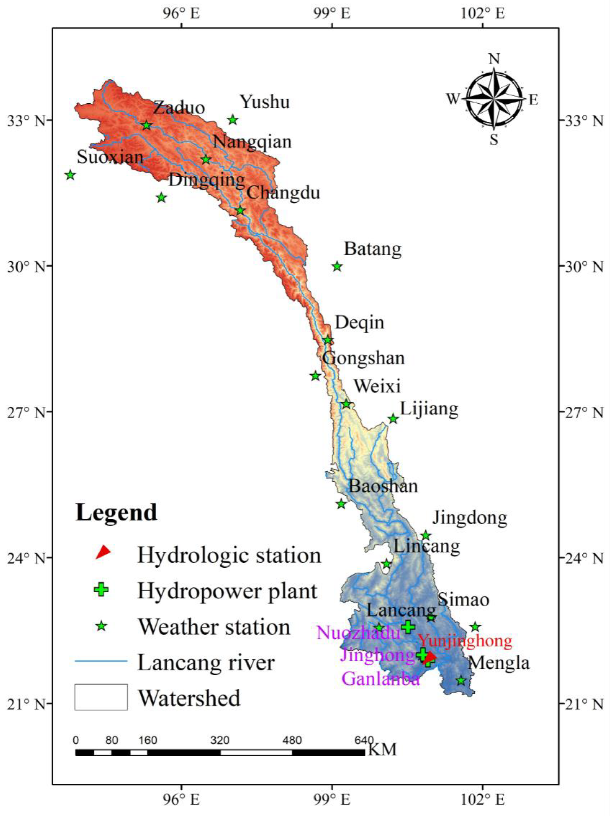
2. Study Area and Data

The Lancang River (Figure 1), as a transboundary river located in the southwest of China, originates in the Qinghai Province of China [47,48,49], and the upper reaches are in China, with the lower reaches flowing through Myanmar and Laos, there called the Mekong River, after exiting from the Yunnan Province. The Lancang River, running through the Hengduan Mountains, is a typical north–south river, and the entire basin has a southwest monsoon climate, where dry and wet seasons are distinct. The main stream is 4880 km long and the watershed area covers 0.81 million km², making it the ninth longest river in the world. The annual mean runoff is 1700 m³/s, annual mean evaporation is 900 mm and the annual mean air temperature is 11 °C. Additionally, the distribution of precipitation is extremely uneven, and from northwest to southeast, the precipitation increases from less than 250 mm to 1600 mm [50]. Generally, May to October is the wet season, covering 85% of the annual mean precipitation, and November to April is the dry season.

The adopted data were divided into hydrological and meteorological data. The meteorological data from 1960 to 2013 of 19 meteorological stations were collected from the National Climatic Centre of China. The daily runoff data from 1960 to 2013 were provided by the Huaneng Lancang River Hydropower Co., Ltd. (Kunming, China), collected from the hydrological station called Yunjinghong in the downstream area, shown in Figure 1.

3. Methods

3.1. CHSH Model

In this study, the BP, NAR, RBF, SVM and TOPMODEL were adopted to construct the CHSH model [51]. The main content in this study focuses on the construction and good performance of the hierarchical structure combination hydrological model, so a detailed description of the single models mentioned above is not provided here.

3.1.1. Model Evaluation

There are many evaluation indexes for the long- and mid-term runoff simulated model, and there is no uniform standard. In this study, based on the simulation accuracy, the simulation stability was added, and both evaluation indexes were adopted to evaluate and analyze the simulation results of the model.

(1)

Simulated accuracy

Simulated accuracy, a type of the most commonly used indexes, measures the pros and cons of the simulated results. In general, the relative error is adopted to measure the simulated results, and the smaller it is, the higher the simulated accuracy. The relative error and accuracy for time interval are shown as Equations (1) and (2), respectively. The overall simulated accuracy of the model is shown in Equation (3):

$$e_i=\frac{\left|Q_i-{\widehat{Q}}_i\right|}{Q_i}$$

(1)

$$A_i=1-e_i$$

(2)

$$e=1-\frac{1}{n}{\displaystyle \sum _{i=1}^n{e}_i}$$

(3)

where $e_i$ represents the relative error for the model at time i; $A_i$ is the simulated accuracy for the model at time i; ${\widehat{Q}}_i$ and $Q_i$ are the simulated value and observed value for the model at time i, respectively; e represents the overall simulated accuracy; and n is the length of the simulated sequence.

(2)

Simulated stability

In the process of runoff simulation, the main task is to improve the simulated stability of the combined model while ensuring the accuracy of the simulation, and the simulated stability is measured by the overall volatility. The overall simulated volatility in this study is mainly related to the relative variations of the simulated results, and the overall volatility of the simulated results change with the relative variations. The overall volatility of the simulated model can be described as follows:

$$E_z=\frac{{\displaystyle \sum _{i=1}^{n-1}{\displaystyle \sum _{j=i+1}^n\sqrt{\left|e_i-e_j\right|}}}}{{\displaystyle \sum _{i=1}^{n}i}}$$

(4)

where $E_z$ represents the overall volatility of the simulated model and e_i and e_j are the relative errors of simulated results at times i and j, respectively.

3.1.2. Model Construction

There are m models that can be merged in the combination simulation of runoff, and the corresponding simulated values are $f_1(t),f_2(t),\dots ,f_i(t)$. Therefore, the simulation of the combination model can be described as follows:

$$f(t)={\displaystyle \sum _{t=1}^T{\displaystyle \sum _{i=1}^m{\omega }_i(t)f_i(t)}}$$

(5)

where $f(t)$ is the combination simulation value at time t; ${\omega }_i(t)$ is the weight for the i-th model at time t; $f_i(t)$ is the simulation value for the i-th model at time t; i represents the index for combination models; t represents the index for time intervals; m represents the total number of the single models; and T represents the total number of time intervals.

For m simulated models ($i=1,2,\dots ,m$), if ${\omega }_i(t)=1/m$, the weights for a single model at each time are the same, and the combination model is a fixed-weight combination simulation (Equation (5)). The determination of the weights in the fixed-weight combination simulation is relatively simple, but it cannot fully explain the positive and negative results that may occur in each single model simulation. Conversely, in the variable-weight combination simulation (${\omega }_i(t)\ne 1/m$), weight changes with time, and the information for the simulation of each single model can be better integrated in the simulated process, being performed more realistically.

After the pre-processing of each single model and obtaining their results, weights are assigned to the final selected models for the combination simulation of runoff. In this study, the step-by-step method for determining the weight of each single model was adopted to establish the combination model with a hierarchical structure. Firstly, the relative weights for each single model (${\omega }_{11},{\omega }_{21},\dots ,{\omega }_{i1}$) under the accuracy index were determined by the variance–covariance optimization combination method. Secondly, the relative weights for each single model (${\omega }_{12},{\omega }_{22},\dots ,{\omega }_{i2}$) under the stability index were determined by the weight method. Thirdly, the relative weights for the two evaluation indexes of simulated accuracy and the stability ($g_1,g_2$) were determined by entropy weight method. Finally, the combination weight coefficient for each single model is shown in Equation (6). The hierarchical combination hydrological model is shown in Figure 2.

$${\omega }_i={\omega }_{i1}{g}_1+{\omega }_{i2}{g}_2 i=1,2,\dots ,I$$

(6)

(1)

Determination of the weight of a single model under simulation accuracy

For the simulation accuracy index, the relative weight for each single model was determined by the variance–covariance optimization combination method. Considering there are m single models, $f_1(t),f_2(t),\cdots ,f_m(t)$ are the simulation results; ${\sigma }_1,{\sigma }_2,\cdots ,{\sigma }_m$ are the variances of the simulation errors, and the errors of the models are not correlated; and ${\omega }_{11},{\omega }_{21},\dots ,{\omega }_{i1}$ are the relative weights of each single model. Thus, the simulation results of m models are as follows:

$$f={\displaystyle \sum _{i=1}^m{\omega }_{i1}{f}_i(t)}$$

(7)

where ${\omega }_{i1}$ is the relative weight for the i-th model (${\displaystyle \sum {\omega }_{i1}}=1$), and the variance for combination simulation is $\sigma (e)={\displaystyle \sum _{i=1}^m{\omega }_{i1}^2{\sigma }_i}$. A Lagrange multiplier is added to $\sigma (e)$ to find the minimum value, and under the constraint of ${\displaystyle \sum _{i=1}^m{\omega }_{i1}}=1$ to obtain ${\omega }_{i1}=1/({\sigma }_1^{-1}+{\sigma }_2^{-1}+\cdot \cdot \cdot +{\sigma }_m^{-1})$. Considering $e_{1t},e_{2t},\cdot \cdot \cdot ,e_{mt}$ are the errors of m single models, when it obeys standard normal distribution (average is 0), the estimate for ${\sigma }_i(t)$ is ${\widehat{\sigma }}_i=\frac{1}{n}{\displaystyle \sum _{t=1}^n{(e_{it})}^2}$, where $t=1,2,\dots ,n$, and n represents the length of historical data. Therefore, the estimate for ${\omega }_{i1}$ can be represented as follows:

$${\widehat{\omega }}_{i1}={({\displaystyle \sum _{t=1}^n{e}_{it}^2})}^{-1}{[{\displaystyle \sum _{j=1}^m{({\displaystyle \sum _{t=1}^n{e}^2{}_{jt}})}^{-1}}]}^{-1}$$

(8)

(2)

Determination of the weight of a single model under simulation stability

The relative weight for each single model was determined by the weight method under the simulation stability index. Considering the overall fluctuations for m, the single simulation models are $v_1,v_2,\cdots v_m$. Therefore, on the contrary, the simulation stabilities for the models are $1-v_1,1-v_2,\cdots ,1-v_m$, respectively. Supposing that the simulation stabilities of the models are independent, the weights ${\omega }_{i2}$ of the models under the simulation stability index were determined by the weighted average method, which is described in Equation (9):

$${\omega }_{i2}=\frac{1-v_i}{{\displaystyle \sum _{i=1}^m(1-v_i)}} i=1,2,\dots ,m$$

(9)

(3)

Determination of the weights of the evaluation indexes

The entropy weight method is objective, and the main idea is to determine the objective weights depending on the variability of indexes. Generally, the smaller the information entropy of an index, the larger the variability degree of the index. On the other hand, a larger the amount of information an index contains, the larger the impact of the index in the comprehensive evaluation, and the larger its weight. In the process of constructing a CHSH model, the relative weights for the evaluation indexes of the simulation accuracy and simulation stability were determined. In this study, the entropy weight method was adopted to determine the relative weights according to the information of model evaluation indexes.

The entropy for the system can be defined as follows:

$$E=-k{\displaystyle \sum _{l=1}^q{p}_l\ln p_l}$$

(10)

where $p_l$ is the probability for appearance of the l-th state and $l=1,2,\dots ,q$, where q is the number for states of probable appearance in the system. Considering there are m single models and s evaluation indexes, in the construction of a combined model, the original data index matrix is $R={(r_{ij})}_{m\times s}$, where r represents the value for the i-th model under the j-th index and $1\le i\le m$ and $1\le j\le s$. From the system entropy (Equation (10)), the entropy for the j-th index is as follows:

$$E_j=-k{\displaystyle \sum _{i=1}^m{p}_{ij}\ln p_{ij}}$$

(11)

The detailed steps for the determination of the weights by the entropy weight method are as follows:

(1)

Due to the inconsistent dimension of each selected index, the original data index matrix $R={(r_{ij})}_{m\times s}$ needs to be standardized. The indexes for simulated accuracy and simulated stability selected in this study were all positive with an attribute of large and excellent, and the standardized equation is ${r_{ij}}^{\prime }=r_{ij}/\underset{j}{max}{r}_{ij}$. The matrix after standardizing is $R^{\prime }={({r^{\prime }}_{ij})}_{m\times s}$, where $i=1,2,\dots ,m$ and $j=1,2,\dots ,s$.

(2)

The proportion $p_{ij}$ for the index values of the i-th simulated method are calculated under the j-th index in the sum of all methods $p_{ij}=r_{ij}^{\prime }/{\displaystyle \sum _{i=1}^m{r}^{\prime }{}_{ij}}$.

(3)

Taking $k=1/\ln m$, using Equations (7)–(11), the j-th index entropy value $E_j$ is calculated, with $0<E_j<1$.

(4)

The j-th index difference coefficient is calculated, $h_j=1-E_j$.

(5)

A value is assigned to each index, and the weight of the j-th index is as follows:

$$g_j=\frac{h_j}{{\displaystyle \sum _{j=1}^s{h}_j}}$$

(12)

3.2. VAR Model

The vector autoregressive model, based on economic theory, was firstly proposed by Christopher Sims [40,41], and it is a widely used model for data statistics. Its aim is to predict and randomly disturb the data series and observe the dynamic response relationship between the variables. Due to the analysis of the dynamic relationship within variables, the VAR model can achieve the research on dynamic transmission mechanism. Recently, it has been widely used in multivariate data analysis.

There are a few restrictive conditions in the process of running the model. Multivariate simultaneous equations are adopted, with the lag of the endogenous variable of each single equation being used to represent the regression variable, and the dynamic relationship between variables is obtained. The mathematical expression is as follows:

$$x_t=a{x}_{t-1}+\cdots a_n{x}_{t-n}+\beta y_t+{\rho }_t\hspace{0.17em}\hspace{0.17em}\hspace{0.17em}\hspace{0.17em}\hspace{0.17em}\hspace{0.17em}\hspace{0.17em}t=1,2,\cdots ,T$$

(13)

where $x_t$ and $y_t$ represent the endogenous variable and exogenous variable, respectively; T is the sample number; n is the lag interval for the endogenous variable; ${\rho }_t$ is a perturbation vector; and $a_n$ and $\beta$ are coefficient matrixes.

The VAR model is mainly used to study the dynamic variety rules for sequences, and its impulse response function is a non-theoretical model, without the need to explain each parameter estimate value when using the model. Therefore, the model emphasizes the significance of the regression coefficients for the equation and focuses on the overall stability of the model without being concerned with parameter tests. Based on the above, the impulse response and variance decomposition were adopted to study the impact and response of the sequence with random disturbances to the entire system. Variance decomposition is a description method of the relative effects to test the impact contribution of each variable update on the variables in the VAR system, and the main idea is to decompose the fluctuation (k-step predicted mean square error) of each endogenous variable (four variables in this article) in the system into m components that are related to each type of equation information according to its causality. Thus, the relative importance of each type of information on the endogenous variables is obtained. In recent years, it has been usually used in the field of hydrology to analyze the contribution rates of precipitation, temperature and other meteorological factors to runoff changes.

The model analysis process is divided into the following steps:

(1)

The Augmented Dickey–Fuller (ADF) method is used to test the unit roots in the sequence to eliminate the phenomenon of spurious regression.

(2)

The lag intervals for the endogenous variables are determined.

(3)

The model coefficient is estimated and the VAR model is constructed.

(4)

The root estimate method is used for stationarity test.

(5)

The impact of a variable or several variables, after considering the impact on the numerical results of other variables in the present and future, is determined by the impulse response function.

(6)

The variance decomposition method is used to conduct dynamic research on the VAR model and analyze the reaction for each variable after being impacted. Concurrently, this is compared with the analysis results of the impulse response so as to test the stability and scientific validity of the model.

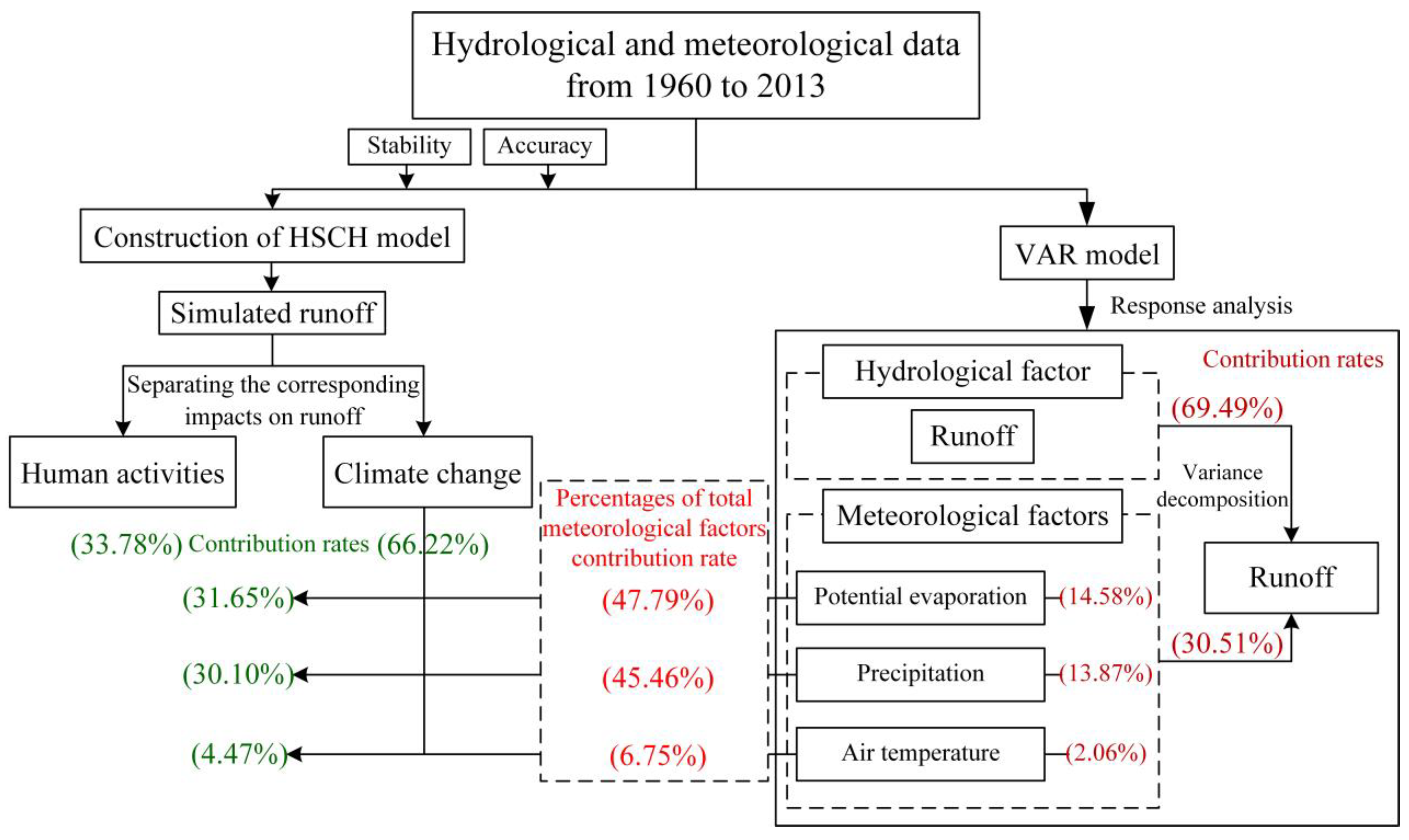
4. Results and Discussion

4.1. Impacts of Human Activities and Climate Change

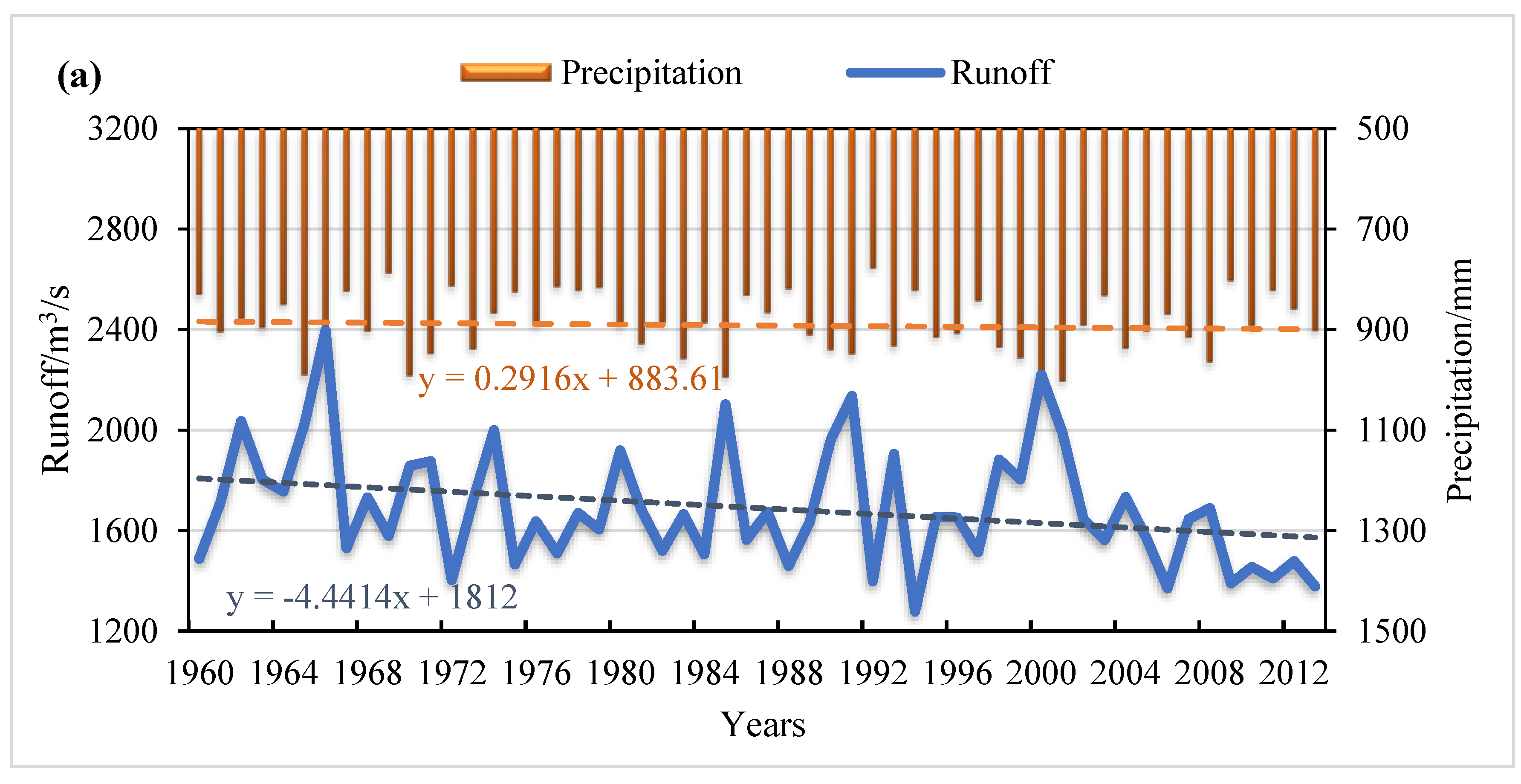
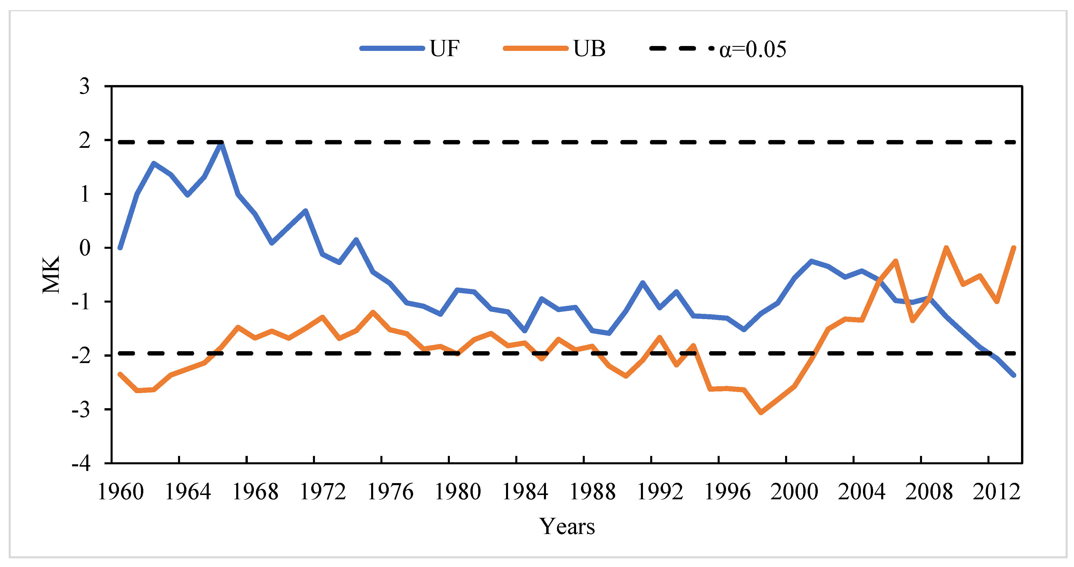
4.1.1. Analysis of Measured Hydro-Meteorological Data

The annual mean runoff and precipitation are shown in Figure 3a. The annual mean runoff of the Lancang River basin is 1690 m³/s; the maximum runoff (2396 m³/s) appeared in 1966 and the minimum (1278 m³/s) in 1994; and the runoff has a decreasing trend of 4.4 m³/s per year. The annual mean precipitation is 892 mm; the maximum (1026 mm) appeared in 2000 and the minimum (778 mm) in 1992; and the precipitation has an increasing trend of 0.29 mm per year. Additionally, the annual mean evaporation and air temperature are shown in Figure 3b. The annual mean potential evaporation is 928 mm calculated with the Penman evapotranspiration formula; the maximum (997 mm) appeared in 2009 and the minimum (844 mm) in 1962; and the potential evaporation has an increasing trend of 1.2 mm per year. The annual mean air temperature is 11 °C; the maximum (13 °C) appeared in 2009 and the minimum (10 °C) in 1968; and the air temperature has an increasing trend of 0.03 °C per year.

The Mann–Kendall method was used to test the abrupt point of the runoff, and Figure 4 shows that noticeable intersections appeared between 2005 and 2008; namely, abrupt runoff points appeared in this period. By searching related information, the construction of the Jinghong hydropower plant started in 2003, while the Nuozhadu hydropower plant was started in 2006. Generally, the construction of a hydropower plant changes the hydrological circulation system of a river, leading to the appearance of an abrupt point in runoff. Duo to the necessary selection of a calibration period and verification period for the single model of TOPMODEL, according to the time period of the abrupt point, the time periods from 1960 to 1985 and from 1986 to 2004 were selected as the calibration period and verification period, respectively.

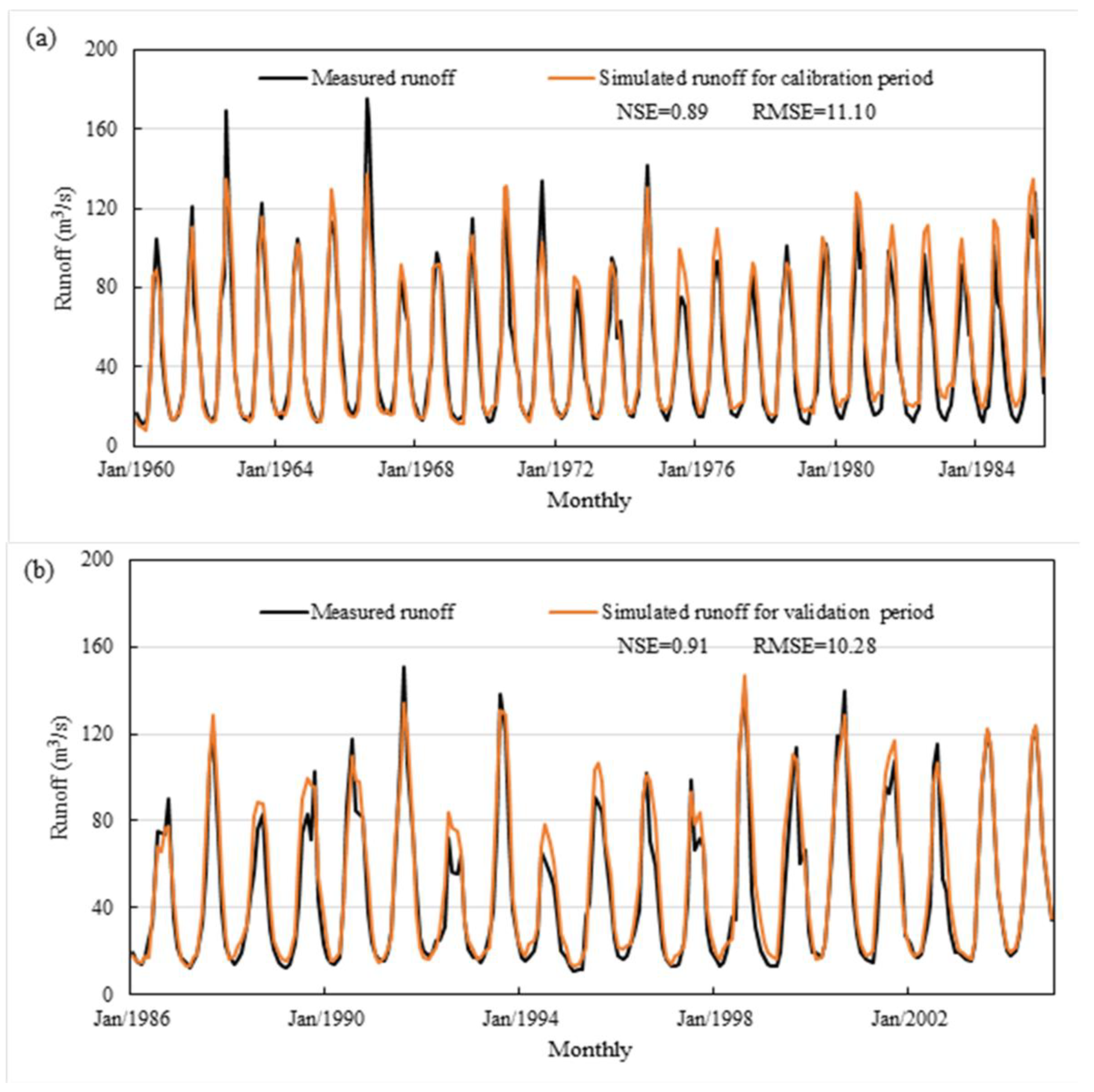
4.1.2. Simulating Natural Runoff by a CHSH Model

According to the runoff data, the runoff abrupt point appeared between 2005 and 2008, with the period of 1960–2004 being considered the natural period and 2005–2013 the human impact period. The data series from 1960 to 2004 was selected as the natural historical data to construct five single models, namely, BP, NAR, RBF, SVM and TOPMODEL, and the monthly runoff from 2005 to 2013 was simulated using the CHSH model.

The measured runoff and simulated runoff for the five simulated models are shown in Figure 5 and Figure 6, respectively, and the corresponding RE, RMSE and NSE for the simulated compared with the measured runoff are shown in

Table 1. Evaluation indexes for the results of the five simulated models.

Indexes	BP	NAR	RBF	SVM	Topmodel
					Calibration Period	Validation Period
RE (%)	16	17	17	14	20	19
RMSE (108 m3)	12	11	12	12	11	10
NSE	0.87	0.89	0.88	0.87	0.89	0.91

. In Table 1, there are no noticeable differences for the NSE between the five models, but the RMSEs for BP and SVM are somewhat higher compared with those of the other three models. TOPMODEL had the lowest RMSE (11 × 10⁸ m³ and 10 × 10⁸ m³), while the RE for SVM was the lowest (14%) and the highest value belonged to TOPMODEL, which in the calibration period was 20% and in the verification period 19%. Overall, the simulated results for the five model were acceptable with high simulated accuracy, which shows that the five selected models have certain advantages in the process of runoff simulation. Moreover, the five models performed excellently for the low-flow part, but the simulated results in some peaks were not as good. Therefore, a better runoff simulated model that integrates the advantages while avoiding the disadvantages of the five models needs to be constructed to achieve the best simulated effect.

The variance–covariance method and the weight method were adopted to determine the weights for five single models under the evaluation indexes of the simulated accuracy and simulated stability, respectively. Concurrently, the relative weights for the evaluation indexes of the simulated accuracy and simulated stability were obtained by the entropy weight method, as shown in

Table 2. Weight for each single model (%).

Indexes	BP	NAR	RBF	SVM	Topmodel
Variance–Covariance	16	17	15	18	34
Weight	20	20	20	20	20
Determined Weigh	16	17	15	18	34

.

After the weights of the single models were determined, they were applied in Equation (5), and the runoff simulated values were calculated, as shown in Figure 7. The simulated monthly runoff from 2005 to 2013 of the CHSH model is close to the measured runoff, and the RE, RMSE and NSE are 6.4%, 6.7 × 10⁸ m³ and 0.94, respectively, which shows the excellent performance for the runoff simulation of the combination model.

4.1.3. Quantification of the Impact of Human Activities and Climate Change on Runoff

In previous studies, the difference ($\Delta R$) between the simulated and measured value during the impact period of human activities has been defined as the contribution of human activities to runoff [35]. According to this method, the measured runoff decrease ${\eta }_R$ was 18% (9.717 billion m³) during the period of human impact (2005–2013) compared with the base period (1960–2004), as shown in

Table 3. Impact of climate change and human activities on runoff based on the CHSH model.

Period	${\mathit{R}}_0$ /108 m3	${\mathit{R}}_{\mathit{S}}$ /108 m3	$\Delta \mathit{R}$ /108 m3	${\mathit{\eta }}_{\mathit{R}}$ /%	Human Activities		Climate Change
					$\Delta {\mathit{R}}_{\mathit{H}}$ /108 m3	${\mathit{\eta }}_{\mathit{H}}$ /%	$\Delta {\mathit{R}}_{\mathit{C}}$ /108 m3	${\mathit{\eta }}_{\mathit{C}}$ /%
1960–2004	545	-	-	-	-	-	-	-
2005–2013	469	495	−77	−14	−26	34	−50	66

, and the phenomenon resulted from the cooperation of climate change and human activities. In the period of human impact, the measured runoff ($R_0$) was lower than the simulated runoff ($R_S$), and the decrease $\Delta R_H$ (2.6 billion m³) was caused by human activities; the contribution rate (to runoff decrease) ${\eta }_H$ was 34%. Additionally, the difference between the simulated runoff during the period of human activities and the measured value during the base period was 5.1 billion m³ ($\Delta R_C$), which is caused by climate change, and the contribution rate (${\eta }_C$) is 66%. In summary, it is concluded that the impact of climate change on runoff is much more than that of human activities.

The method to separate the impacts of human activities and climate change is not meticulous. Moreover, the results are dependent on the simulation accuracy of the model, and the calculated proportion of human activities decreases as the simulation accuracy increases. Therefore, this method cannot truly represent the actual situation. In the following part, the VAR model is proposed to quantitatively analyze the impact of climate change on runoff.

4.2. Separating the Impact of Each Meteorological Factor on Runoff

4.2.1. Construction of the VAR Model

In this study, the ADF method was adopted to test the stability of the sequence, that is, whether there is a unit root in the sequence, and if so, this leads to the phenomenon of spurious regression during the regression analysis. In the process of the ADF test, the null hypothesis is that there is a unit root in the sequence, which means that the sequence belongs to non-stationary series. If the ADF value is larger than the critical value, the sequence is considered as a non-stationary series; otherwise, the null hypothesis is not accepted. In

Table 4. Results of the ADF test of each factor.

Variable	ADF Test		Critical Value (α = 5%)		Result
	t-Statistic	p-Value	t-Statistic	p-Value
Q	−4.5 *	0.0002	−2.9	0.05	Stationary
P	−5.8 *	0	−2.9	0.05	Stationary
T	−3.1 *	0.029	−2.9	0.05	Stationary
E	−3.2 *	0.022	−2.9	0.05	Stationary

Note: * at the significance level of 95%, the null hypothesis is rejected. Here, Q, P, T and E stand for runoff, precipitation, air temperature and potential evaporation, respectively.

, the results show that all four factors rejected the null hypothesis, which means that the four groups of data from 1960 to 2013 are stationary series. Therefore, it is concluded that the four groups of factor sequences reach the conditions of the VAR model.

One of the most necessary steps for the estimation of the VAR model is to determine the lag phase, and the lag period means that the impact appears in some time instead of appears immediately. In this study, the unit of lag is a month (all the hydro-meteorological factor sequences are one month). In order to fully reflect the dynamic properties of the constructed model, it is necessary to ensure that the order of the lag period is sufficiently large. However, too many lag periods will increase the number of estimated parameters, and insufficient lag periods will decrease the degree of freedom of the model, affecting the effectiveness of the parameters estimated by the model.

In this study, the five statistics Likelihood Ratio (LR), Final Prediction Error Criterian (FPE), Akaike Information Criterion (AIC), Schwarz Criterion (SC) and Hannan-Quinn Criterion (HQ) were selected to determine the best lag period [52,53]. The calculated results for the lag periods of the four factors are shown in

Table 5. Results of the lag length test for the VAR model constructed by four groups of hydro-meteorological factors.

Lag	LogL	LR	FPE	AIC	SC	HQ
0	−611	NA	7.9 × 10−5	1.9	1.9	1.9
1	−3. 3	1207	1.3 × 10−5	0.072	0.21	0.13
2	302	601*	5.2 × 10−6 *	−0.83 *	−0.58 *	−0.73 *
3	514	416	2.8 × 10−6	−1.4	−1.1	−1.3

Note: * the best lag order under the statistical criteria. LogL is the logarithm of Lag.

. From Table 5, it can be observed that all five statistics approached the best values when the lag period was 2. Therefore, the best lag period for the VAR model that was constructed by the four groups of hydro-meteorological factors was 2.

The coefficients of the VAR model were estimated after the best lag period was determined. The VAR model was constructed with the sequence of runoff, precipitation, potential evaporation and air temperature, and the coefficients for the model are shown in

Table 6. Coefficients for the VAR model constructed by hydro-meteorological factors.

Statistics	Q	P	E	T
Q (-1)	0.27	−0.015	0.078	0.0075
Q (-2)	−0.20	−0.77	−0.14	−0.018
P (-1)	0.27	0.38	0.068	0.016
P (-2)	0.094	0.23	−0.0094	0.0012
E (-1)	−0.21	0.37	0.67	0.082
E (-2)	0.29	1.2	0.15	0.012
T (-1)	1.8	1.6	2.0	0.63
T (-2)	−1.7	−2.9	−4.7	−0.54
C	6.7	−47	43	2.2
R2	0.84	0.81	0.90	0.99

Note: P, Q, E and T represent precipitation, runoff, potential evaporation and air temperature, respectively, and the values in brackets represent lag length.

. The runoff sequence was selected as a case for analysis, with an R² value of 0.84. The coefficients for the impact of runoff, precipitation, potential evaporation and air temperature in the 1-lag period on the current runoff were, respectively, 0.27, −0.015, 0.078 and 0.0075, while the corresponding coefficients for the 2-lag period on the current runoff were −1.2, −0.77, −0.14 and −0.018, respectively. Similarly, the R² for the sequence of precipitation, potential evaporation and air temperature were 0.81, 0.90 and 0.99, respectively, which shows that the goodness of fit for all factors was good. The coefficients for the impact of the other three factors in the 1-lag and 2-lag periods on each other are shown in Table 6.

4.2.2. Stationarity Test of the VAR Model

To avoid invalid results due to model instability, the most important task is to estimate the stationarity of the constructed VAR model. Therefore, the unit root estimation method was adopted to test the stationarity of the VAR model, that is, the modulus reciprocals of all the unit roots are in the unit circle (radius is 1), which means the constructed model reaches the stationarity standard to continue with further analysis for impulse response and variance decomposition.

The two-order VAR model constructed by four groups of factors was processed by the unit root test, as shown in Figure 8. It was concluded that the root modulus reciprocals of all the characteristic polynomials were in the unit circle, which means that the VAR model reaches the stationarity standard.

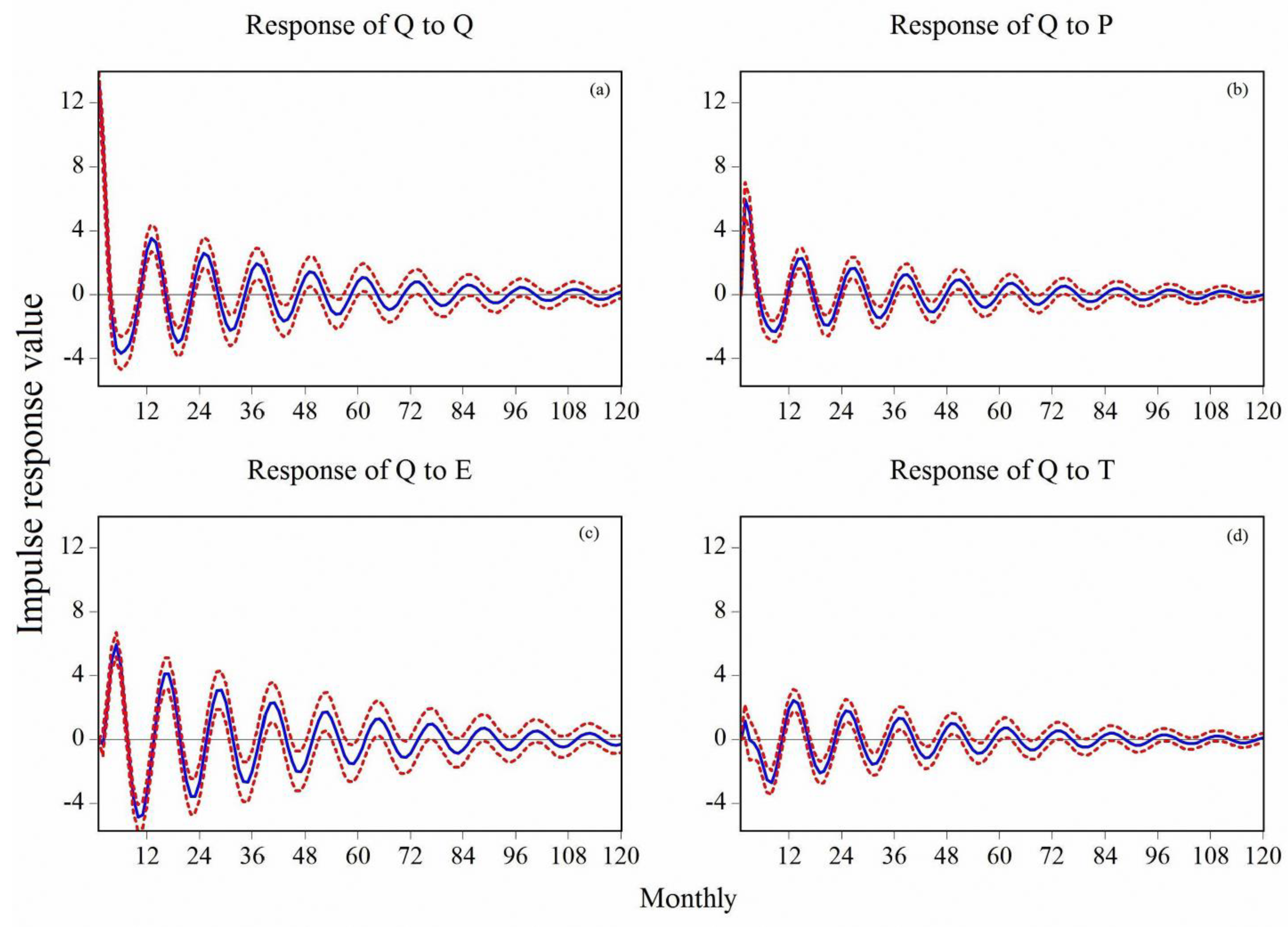
4.2.3. Impulse Response of Runoff to the Meteorological Factors

When one variable in the system changes with a certain fluctuation, it will inevitably have a corresponding impact on itself or other related variables. In this study, the impulse response function (IRF) was adopted to quantify this type of relationship, aiming to provide a standard deviation impulse to a random disturbance item in the system to measure the response or variation for the values of all endogenous variables in the future, including changes, degrees, persistence and pulsation. Using IRF can intuitively describe the dynamic interaction response and effects among all variables [54,55].

The impulse response theory was used to analyze the dynamic interaction response, and we selected the lag of 120 months (10 years) to simulate the response tracts of the four groups of factors. IRF was mainly used to observe the time lengths of the variables with a fluctuation tending to stability.

The impulse response results for runoff, precipitation, potential evaporation and air temperature to runoff are shown in Figure 9, and the impulse response curve and the curves of impulse response curve superimposed with one standard deviation showed convergence. It is obviously concluded that the long-term response gradually weakened, tending to 0, which means that a standard deviation impulse for the four groups of factors have a strong impact to runoff. Furthermore, in addition to runoff having quite a strong fluctuation response to itself, it responded to the changes in precipitation and potential evaporation, which, in the transmission process, showed a volatility response. In the first period, in addition to runoff not responding to air temperature variations, runoff had a strong positive response to changes in itself and precipitation (response values of 9.3 and 8.7, respectively), and regarding potential evaporation, it showed a strong negative response (response value of −3.6), but the response amplitude gradually decreased and the volatility became increasingly weaker.

The impact of the three climatic factors on runoff shows that the mean response value of runoff to precipitation was positive (response value of 0.53), which means that the increasing precipitation promotes the increase in runoff. However, the response values of runoff to potential evaporation and air temperature were negative (response values of −0.07 and −0.24, respectively), meaning the increases in potential evaporation and air temperature inhibit the increase in runoff. Of the three climatic factors, the impact of the precipitation and potential evaporation on runoff at the beginning was noticeable, and the wave shape appeared as a gradually weakening sine curve. The strongest negative and positive response values were, respectively, (−4.4, 10) and (−4.5, 6.4), as shown in Figure 9b,c. Additionally, the impact of the air temperature on runoff was not very evident, and the range was (−2.7–2.5).

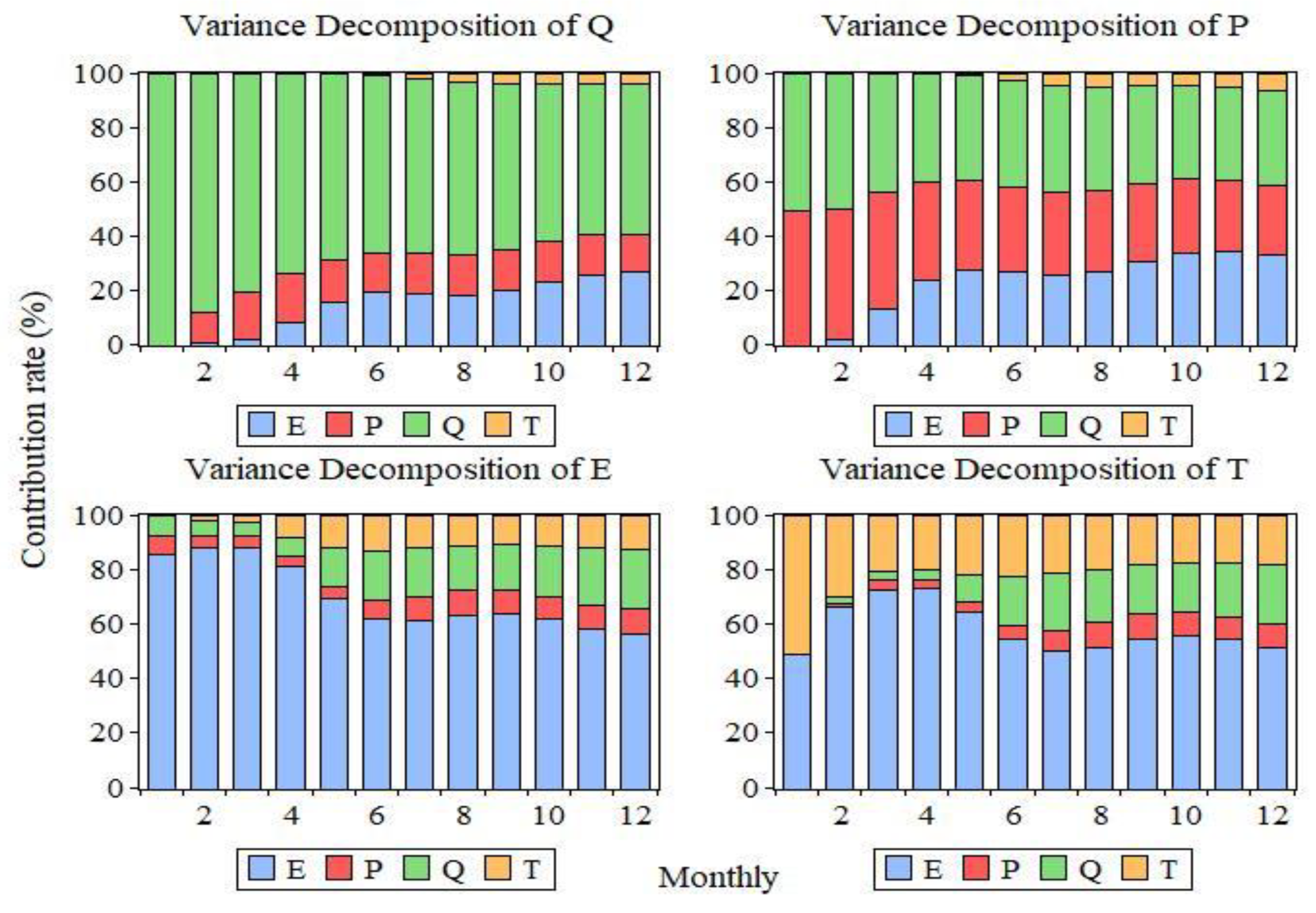
4.2.4. Analysis of the Contribution Rates of the Meteorological Factors to Runoff

The variance decomposition method was adopted to quantitatively estimate the contribution rates of hydro-meteorological factors to runoff changes. However, different from IRF, the contribution of each endogenous variable in the system to the total can be calculated using the variance decomposition method.

Considering the lag as 12 months (one year), the independent variables were precipitation, potential evaporation and air temperature, and the dependent variable was runoff. The results of the contribution rates of runoff by variance decomposition at a lag of 12 months are shown in

Table 7. Contribution rate of runoff by variance decomposition (%).

Lag	Q	P	E	T
1	100	0	0	0
2	88	12	0.030	0.45
3	80	18	1.6	0.40
4	74	18	8.1	0.37
5	68	17	16	0.44
6	65	15	19	0.96
7	65	15	18	2.2
8	63	15	18	3.5
9	61	15	20	4.1
10	58	15	23	4.0
11	56	15	26	3.9
12	55	14	27	4.4
Average	69	14	15	2.1

, and at the lag of the first month, the contribution of runoff to itself was 100%, but for other variables, there was no contribution. From lag of the second month, precipitation, potential evaporation and air temperature started to contribute to runoff, and considering the mean contribution rate, in addition to the runoff itself, precipitation and potential evaporation had a slight change (contribution rates of 15% and 14%, respectively), while air temperature had a small contribution to runoff (contribution rate of only 2%). It was found from the different results that the contribution rate of precipitation to runoff changes little and ranges from 12% to 18% (no contribution in the first month), while the contribution rate of potential evaporation to runoff gradually increases, with a notable variation amplitude in the second month, and the contribution rate reaches a peak of 27%. Additionally, the contribution rate of air temperature to runoff is within 1% in the first 6 months, and the peak is only 4.4%.

The interaction of the four hydro-meteorological factors is shown in Figure 10, and it can be concluded that, of the four factors, runoff had the greatest impact on itself and precipitation; potential evaporation had the greatest impact on itself and air temperature; and the impact of precipitation on itself ranked second—it had the greatest impact on air temperature. The contribution rates of precipitation and potential evaporation to runoff were both about 14%, and air temperature was about 2%. For precipitation, the contribution rate of runoff to precipitation was dominant (40%), and the contribution rate of potential evaporation was about 23%, with that of air temperature being the lowest (only 3%). For potential evaporation, the contribution rates of runoff, precipitation and air temperature were, respectively, 14%, 7% and 9%, and the contribution rate of air temperature to potential evaporation increased notably compared with that of air temperature to runoff and precipitation. For air temperature, the contribution rates of runoff and precipitation were 13% and 5.6%, lower than to itself. Figure 11 presents the process graph for dynamic response of the hydro-meteorological factors (line width represents the contribution rate), with the contribution directions and amounts being shown clearly.

Table 7 shows that runoff had the largest contribution to itself (the average contribution rate was 69%), so the contribution rate of meteorological factors was 31%. Additionally, the runoff response was mainly from the effects of potential evaporation and precipitation, and the corresponding contribution rate was 15% and 14%, respectively, accounting for 48% and 46% of the total contribution of climate variation, much higher than that of air temperature (2%), accounting for 6.8%. Therefore, based on results of the impact of climate variation and human activities on runoff in Table 3, the contribution rates of potential evaporation, precipitation and air temperature on runoff were 32%, 30% and 4.5%, respectively (shown in

Table 8. Contribution rates of meteorological factors to runoff.

Response for Runoff	Human Activities $\Delta {\mathit{R}}_{\mathit{H}}$	$\mathbf{Climate} \mathbf{Variation} \Delta {\mathit{R}}_{\mathit{C}}$
		$\Delta {\mathit{R}}_{\mathit{E}}$	$\Delta {\mathit{R}}_{\mathit{P}}$	$\Delta {\mathit{R}}_{\mathit{T}}$
Variation/108 m3	−26	−24	−23	−3.4
Contribution rate/%	34	32	30	4.5

), in the Lancang River of China in the period of 2005–2013.

Figure 12 shows the impact of human activities and climate change on runoff by the CHSH model, and the contribution rates for human activities and total climate change were 34% and 66%, respectively. To further separate the contribution rates of the meteorological factors to runoff, the VAR model was constructed and, by the variance decomposition method, the impact of hydrological and meteorological factors on runoff were 69% and 31%, respectively. Among the meteorological factors, the contribution rates of potential evaporation, precipitation and air temperature were 15%, 14% and 2%, accounting for 48%, 45% and 6.8%, respectively. Therefore, the impact of climate change on runoff (contribution rate of 66%) is divided into 32% (for potential evaporation), 30% (for precipitation) and 4.5% (for air temperature), as shown in Figure 12.

5. Conclusions

Runoff, as a part of the water cycle, has an important position in balancing water resources as well as socio-economic benefits. In this paper, to simulate runoff more accurately and to avoid the drawbacks created by simulated single models, a CHSH model was constructed by adding an index of simulation stability based on the simulation accuracy to explore its excellent performance both on accuracy and stability for each single model in runoff simulation. Additionally, against the background of climate change and human activities having an increasingly serious impact on runoff, and moving away from the traditional method of separating the impact of climate change and human activities on runoff, the VAR model was innovatively introduced to separate and analyze the dynamic impact and contribution rate of each meteorological factor (precipitation, potential evaporation and air temperature) on runoff more accurately and clearly.

Based on the indexes of simulation accuracy and simulation stability, the five single models of BP, NAR, RBF, SVM and TOPMODEL were selected to construct the CHSH model to simulate runoff, and the RE, RMSE and NSE were 6.4%, 6.7 × 10⁸ m³ and 0.94, respectively, which shows the good performance of this combination model in runoff simulation. Based on the traditional method of quantitatively analyzing the impact of human activities and climate change on runoff, the contribution rates of human activities and climate change to runoff were calculated by the CHSH model (34% and 66%, respectively). The result of hydrological modeling shows that runoff is more sensitive to the changes in precipitation than changes in potential evaporation.

The VAR model was adopted to quantitatively analyze the impact of each meteorological factor on runoff. The impulse analysis showed convergence and the long-term response gradually weakened, tending to 0, indicating that a standard deviation impulse for the four groups of factors has a strong response to runoff changes. In addition, it was concluded from the results of the response of runoff to the three climatic factors that runoff has a positive response to precipitation variations but has a negative response to the changes in potential evaporation and air temperature.

The results of the variance decomposition analysis for the VAR model show that, for precipitation, the mean contribution rates of potential evaporation, runoff and air temperature are 23%, 20% and 2.6%, respectively; for potential evaporation, the mean contribution rates of runoff, air temperature and precipitation are 12%, 8.2% and 2.0%, respectively; for air temperature, the mean contribution rates of potential evaporation, runoff and precipitation are 29%, 13% and 2.0%, respectively; and for runoff, the mean contribution rates of potential evaporation, air temperature and precipitation are 15%, 14% and 2%, respectively. As a result, according to the results of the impact of climate variation and human activities on runoff, the contribution rates of potential evaporation, precipitation and air temperature on runoff are 32%, 30% and 4.5%, respectively, in the Lancang River of China in the period of 2005–2013.

References

1. Sivapalan, M. Debates-Perspectives on socio-hydrology: Changing water systems and the “tyranny of small problems”-Sociohydrology. Water Resour. Res. 2015, 51, 4795–4805. [Google Scholar] [CrossRef]
2. Liu, D.; Tian, F.; Lin, M.; Sivapalan, M. A conceptual socio-hydrological model of the co-evolution of humans and water: Case study of the Tarim River basin, western China. Hydrol. Earth Syst. Sci. 2015, 19, 1035–1054. [Google Scholar] [CrossRef]
3. Lu, Y.; Tian, F.; Guo, L.; Borzi, I.; Patil, R.; Wei, J.; Liu, D.; Wei, Y.; Yu, D.; Sivapalan, M. Socio-hydrologic modeling of the dynamics of cooperation in the transboundary Lancang-Mekong River. Hydrol. Earth Syst. Sci. 2021, 25, 1883–1903. [Google Scholar] [CrossRef]
4. Alinezhad, A.; Gohari, A.; Eslamian, S.; Saberi, Z. A probabilistic Bayesian framework to deal with the uncertainty in hydro-climate projection of Zayandeh-Rud River Basin. Theor. Appl. Climatol. 2021, 144, 1–14. [Google Scholar] [CrossRef]
5. Meles, M.B.; Goodrich, D.C.; Gupta, H.V.; Burns, I.S.; Unkrich, C.L.; Razavi, S.; Guertin, D.P. Multi-criteria, time dependent sensitivity analysis of an event-oriented, physically-based, distributed sediment and runoff model. J. Hydrol. 2021, 598, 126268. [Google Scholar] [CrossRef]
6. Cheng, C.-T.; Xie, J.-X.; Chau, K.-W.; Layeghifard, M. A new indirect multi-step-ahead prediction model for a long-term hydrologic prediction. J. Hydrol. 2008, 361, 118–130. [Google Scholar] [CrossRef]
7. Kennedy, A.M.; Garen, D.C.; Koch, R.W. The association between climate teleconnection indices and Upper Klamath seasonal streamflow: Trans-Niño Index. Hydrol. Process. 2009, 23, 973–984. [Google Scholar] [CrossRef]
8. Mutlu, E.; Chaubey, I.; Hexmoor, H.; Bajwa, S.G. Comparison of artificial neural network models for hydrologic predictions at multiple gauging stations in an agricultural watershed. Hydrol. Process. 2008, 22, 5097–5106. [Google Scholar] [CrossRef]
9. Sibtain, M.; Li, X.; Azam, M.I.; Bashir, H. Applicability of a Three-Stage Hybrid Model byEmploying a Two-Stage Signal DecompositionApproach and a Deep Learning Methodologyfor Runoff Forecasting at Swat River Catchment,Pakistan. Pol. J. Environ. Stud. 2020, 30, 369–384. [Google Scholar] [CrossRef]
10. Rajesh, R.; Rajendran, C. Grey- and rough-set-based seasonal disaster predictions: An analysis of flood data in India. Nat. Hazards 2019, 97, 395–435. [Google Scholar] [CrossRef]
11. Chen, X.; Wang, X.; Lian, J. Applicability Study of Hydrological Period Identification Methods: Application to Huayuankou and Lijin in the Yellow River Basin, China. Water 2021, 13, 1265. [Google Scholar] [CrossRef]
12. Han, H.; Morrison, R.R. Data-driven approaches for runoff prediction using distributed data. Stoch. Environ. Res. Risk A 2021, 36, 2153–2171. [Google Scholar] [CrossRef]
13. Emerton, R.E.; Stephens, E.M.; Cloke, H.L. What is the most useful approach for forecasting hydrological extremes during El Niño. Environ. Res. Commun. 2019, 1, 31002. [Google Scholar] [CrossRef]
14. Wei, B.; Xie, N. Parameter estimation for grey system models: A nonlinear least squares perspective. Commun. Nonlinear Sci. 2021, 95, 105653. [Google Scholar] [CrossRef]
15. Ma, C.; Xu, R.; He, W.; Xia, J. Determining the limiting water level of early flood season by combining multiobjective optimization scheduling and copula joint distribution function: A case study of three gorges reservoir. Sci. Total Environ. 2020, 737, 139789. [Google Scholar] [CrossRef] [PubMed]
16. Xie, M.; Zhou, J.; Li, C.; Zhu, S. Long-term generation scheduling of Xiluodu and Xiangjiaba cascade hydro plants considering monthly streamflow forecasting error. Energ. Convers. Manag. 2015, 105, 368–376. [Google Scholar] [CrossRef]
17. Regonda, S.K.; Rajagopalan, B.; Clark, M.; Zagona, E. A multimodel ensemble forecast framework: Application to spring seasonal flows in the Gunnison River Basin. Water Resour. Res. 2006, 42, 764–777. [Google Scholar] [CrossRef]
18. Shamseldin, A.Y.; O’Connor, K.M.; Liang, G.C. Methods for combining the outputs of different rainfall–runoff models. J. Hydrol. 1997, 197, 203–229. [Google Scholar] [CrossRef]
19. Georgakakos, K.P.; Seo, D.J.; Gupta, H.; Schaake, J.; Butts, M.B. Towards the characterization of streamflow simulation uncertainty through multimodel ensembles. J. Hydrol. 2004, 298, 222–241. [Google Scholar] [CrossRef]
20. Xie, T.; Zhang, G.; Hou, J.; Xie, J.; Lv, M.; Liu, F. Hybrid forecasting model for non-stationary daily runoff series: A case study in the Han River Basin, China. J. Hydrol. 2019, 577, 123915. [Google Scholar] [CrossRef]
21. Zhang, J.; Li, H.; Sun, B.; Fang, H. Multi-time scale co-integration forecast of annual runoff in the source area of the Yellow River. J. Water Clim. Chang. 2021, 12, 101–115. [Google Scholar] [CrossRef]
22. Zhang, L.; Huang, Q.; Liu, D.; Deng, M.; Zhang, H.; Pan, B.; Zhang, H. Long-term and mid-term ecological operation of cascade hydropower plants considering ecological water demands in arid region. J. Clean. Prod. 2021, 279, 123599. [Google Scholar] [CrossRef]
23. Mo, C.; Ruan, Y.; Xiao, X.; Lan, H.; Jin, J. Impact of climate change and human activities on the baseflow in a typical karst basin, Southwest China. Ecol. Indic. 2021, 126, 107628. [Google Scholar] [CrossRef]
24. Su, X.; Li, X.; Niu, Z.; Wang, N.; Liang, X. A new complexity-based three-stage method to comprehensively quantify positive/negative contribution rates of climate change and human activities to changes in runoff in the upper Yellow River. J. Clean. Prod. 2021, 287, 125017. [Google Scholar] [CrossRef]
25. Tang, Y.; Wang, Z. Derivation of the relative contributions of the climate change and human activities to mean annual streamflow change. J. Hydrol. 2021, 595, 125740. [Google Scholar] [CrossRef]
26. Alifujiang, Y.; Abuduwaili, J.; Groll, M.; Issanova, G.; Maihemuti, B. Changes in intra-annual runoff and its response to climate variability and anthropogenic activity in the Lake Issyk-Kul Basin, Kyrgyzstan. Catena 2021, 198, 104974. [Google Scholar] [CrossRef]
27. Yang, G.; Guo, S.; Liu, P.; Block, P. Integration and Evaluation of Forecast-Informed Multiobjective Reservoir Operations. J. Water Res. Plan. Manag. 2020, 146, 4020038. [Google Scholar] [CrossRef]
28. Athar, H.; Nabeel, A.; Nadeem, I.; Saeed, F. Projected changes in the climate of Pakistan using IPCC AR5-based climate models. Theor. Appl. Climatol. 2021, 145, 567–584. [Google Scholar] [CrossRef]
29. Iturbide, M.; Gutiérrez, J.M.; Alves, L.M.; Bedia, J.; Cerezo-Mota, R.; Cimadevilla, E.; Cofiño, A.S.; Luca, A.D.; Faria, S.H.; Gorodetskaya, I.V.; et al. An update of IPCC climate reference regions for subcontinental analysis of climate model data: Definition and aggregated datasets. Earth Syst. Sci. Data 2020, 12, 2959–2970. [Google Scholar] [CrossRef]
30. Makarigakis, A.K.; Jimenez-Cisneros, B.E. UNESCO’s Contribution to Face Global Water Challenges. Water 2019, 11, 388. [Google Scholar] [CrossRef] [Green Version]
31. Saurral, R.I. The hydrologic cycle of the La Plata Basin in the WCRP-CMIP3 multimodel dataset. J. Hydrometeorol. 2010, 11, 1083–1102. [Google Scholar] [CrossRef]
32. de Jong, P.; Barreto, T.B.; Tanajura, C.A.; Oliveira-Esquerre, K.P.; Kiperstok, A.; Torres, E.A. The Impact of Regional Climate Change on Hydroelectric Resources in South America. Renew. Energ. 2021, 173, 76–91. [Google Scholar] [CrossRef]
33. Huq, E.; Abdul-Aziz, O.I. Climate and land cover change impacts on stormwater runoff in large-scale coastal-urban environments. Sci. Total Environ. 2021, 778, 146017. [Google Scholar] [CrossRef] [PubMed]
34. Liu, J.; Zhou, Z.; Yan, Z.; Gong, J.; Jia, Y.; Xu, C.-Y.; Wang, H. A new approach to separating the impacts of climate change and multiple human activities on water cycle processes based on a distributed hydrological model. J. Hydrol. 2019, 578, 124096. [Google Scholar] [CrossRef]
35. Chang, J.; Zhang, H.; Wang, Y.; Zhu, Y. Assessing the impact of climate variability and human activities on streamflow variation. Hydrol. Earth Syst. Sci. 2016, 20, 1547–1560. [Google Scholar] [CrossRef]
36. Chang, J.; Zhang, H.; Wang, Y.; Zhang, L. Impact of climate change on runoff and uncertainty analysis. Nat. Hazards 2017, 88, 1113–1131. [Google Scholar] [CrossRef]
37. Chaudhari, S.; Felfelani, F.; Shin, S.; Pokhrel, Y. Climate and anthropogenic contributions to the desiccation of the second largest saline lake in the twentieth century. J. Hydrol. 2018, 560, 342–353. [Google Scholar] [CrossRef]
38. Silva, A.T.; Portela, M.M. Using Climate-Flood Links and CMIP5 Projections to Assess Flood Design Levels Under Climate Change Scenarios: A Case Study in Southern Brazil. Water Resour. Manag. 2018, 32, 4879–4893. [Google Scholar] [CrossRef]
39. Wu, H.; Liu, D.; Hao, M.; Li, R.; Yang, Q.; Ming, G.; Liu, H. Identification of Time-Varying Parameters of Distributed Hydrological Model in Wei River Basin on Loess Plateau in the Changing Environment. Water 2022, 14, 4021. [Google Scholar] [CrossRef]
40. Sims, C.A. Macroeconomics and reality. Econometrica 1980, 48, 1–48. [Google Scholar] [CrossRef] [Green Version]
41. Sims, C.A.; Stock, J.H.; Watson, M.W. Inference in Linear Time Series Models with Same Unit Roots. Econometrica 1990, 58, 113–144. [Google Scholar] [CrossRef]
42. Fathian, F.; Fakheri-Fard, A.; Modarres, R.; Van Gelder, P.H. Regional scale rainfall-runoff modeling using varx-mgarch approach. Stoch. Environ. Res. Risk A 2018, 33, 407–425. [Google Scholar] [CrossRef]
43. Zeng, W.; Song, S.; Kang, Y.; Gao, X.; Ma, R. Response of runoff to meteorological factors based on time-varying parameter vector autoregressive model with stochastic volatility in arid and semi-arid area of weihe river basin. Sustainability 2022, 14, 6989. [Google Scholar] [CrossRef]
44. Li, G.; Lei, Y.; Ge, J.; Wu, S. The Empirical Relationship between Mining Industry Development and Environmental Pollution in China. Int. J. Environ. Res. Public Health 2017, 14, 254. [Google Scholar] [CrossRef]
45. Wu, S.; Li, J.; Zhou, W.; Lewis, B.J.; Yu, D.; Zhou, L.; Jiang, L.; Dai, L. A statistical analysis of spatiotemporal variations and determinant factors of forest carbon storage under China’s Natural Forest Protection Program. J. Forestry Res. 2018, 29, 415–424. [Google Scholar] [CrossRef]
46. Zhao, J.; Mu, X.; Gao, P. Dynamic response of runoff to soil and water conservation measures and precipitation based on VAR model. Hydrol. Res. 2019, 50, 837–848. [Google Scholar] [CrossRef]
47. Deng, J.; Li, Y.; Xu, B.; Ding, W.; Zhou, H.; Schmidt, A. Ecological Optimal Operation of Hydropower Stations to Maximize Total Phosphorus Export. J. Water Res. Plan. Manag. 2020, 146, 4020075. [Google Scholar] [CrossRef]
48. Zhang, H.; Chang, J.; Gao, C.; Wu, H.; Wang, Y.; Lei, K.; Long, R.; Zhang, L. Cascade hydropower plants operation considering comprehensive ecological water demands. Energ. Convers. Manag. 2019, 180, 119–133. [Google Scholar] [CrossRef]
49. Zhong, R.; Zhao, T.; He, Y.; Chen, X. Hydropower change of the water tower of Asia in 21st century: A case of the Lancang River hydropower base, upper Mekong. Energy 2019, 179, 685–696. [Google Scholar] [CrossRef]
50. Shi, W.; Yu, X.; Liao, W.; Wang, Y.; Jia, B. Spatial and temporal variability of daily precipitation concentration in the Lancang River basin, China. J. Hydrol. 2013, 495, 197–207. [Google Scholar] [CrossRef]
51. Kirkby, M.; Beven, K. A physically based, variable contributing area model of basin hydrology. Hydrol. Sci. J. 1979, 24, 43–69. [Google Scholar]
52. Karimi, M. Order selection criteria for vector autoregressive models. Signal Process. 2011, 91, 955–969. [Google Scholar] [CrossRef]
53. Santosa, B.J. Differential evolution adaptive metropolis sampling method to provide model uncertainty and model selection criteria to determine optimal model for Rayleigh wave dispersion. Arab. J. Geosci. 2015, 8, 7003–7023. [Google Scholar]
54. Ahking, F.W. Model mis-specification and Johansen’s co-integration analysis: An application to the US money demand. J. Macroecon. 2002, 24, 51–66. [Google Scholar] [CrossRef]
55. Lütkepohl, H. A note on the asymptotic distribution of impulse response functions of estimated var models with orthogonal residuals. J. Econom. 1989, 42, 371–376. [Google Scholar] [CrossRef]
Figure 1. The watershed of the Lancang River.
Agronomy 13 00510 g001
Figure 2. The structure diagram for the weight determination of runoff simulation using the CHSH model.
Agronomy 13 00510 g002
Figure 3. Hydrological and meteorological data of the Lancang River basin (1960−2013). (a) Hydrological data and (b) meteorological data.
Agronomy 13 00510 g003aAgronomy 13 00510 g003b
Figure 4. The abrupt point test for runoff of the Nuozhadu Reservoir.
Agronomy 13 00510 g004
Figure 5. Simulated runoff based on the BP, NAR, RBF and SVM models in the training period.
Agronomy 13 00510 g005
Figure 6. Simulated runoff based on the TOPMODEL model. (a) Calibration period and (b) validation period.
Agronomy 13 00510 g006
Figure 7. Results for the runoff simulation of the CHSH model.
Agronomy 13 00510 g007
Figure 8. Stationarity test based on the VAR model constructed by four groups of factors.
Agronomy 13 00510 g008
Figure 9. Impulse response curves of runoff.
Agronomy 13 00510 g009
Figure 10. Mutual contribution rate of the four groups of hydro-meteorological factors.
Agronomy 13 00510 g010
Figure 11. Process graph for the dynamic response of the four groups of hydro-meteorological factors (Q, P, E and T represent runoff, precipitation, potential evaporation and air temperature, respectively).
Agronomy 13 00510 g011
Figure 12. Process of separating the contribution rates of meteorological factors to runoff.
Agronomy 13 00510 g012