Abstract
South Italy is characterised by a semi-arid climate with scarce rain and high evaporative demand. Since climate change could worsen this condition, the need to optimise water resources in this area is crucial. In citrus cultivation, which involves one of the most important crops bred in Southern Italy, and more generally in Mediterranean regions, deficit irrigation strategies are implemented in order to cope with limited resource availability. On this basis, knowledge on how the territorial distribution of citrus would change in relation to these strategies represents valuable information for stakeholders. Therefore, the objective of this study was to determine the probability of the presence of citrus in Sicily based on changes in the percentage of water deficit in order to identify and analyse change in the surface area as well as the location of the crop. The methodology was based on the application of species distribution models (SDM) and Geographic Information Systems (GIS) to the case study of the province of Syracuse in Sicily. Different geostatistical and machine learning models were applied based on bioclimatic variables measured over three decades, a Digital Terrain Model and irrigation. Assessment of the outcomes was carried out using classification evaluation metrics. The analysis of the outcomes showed that uncorrelated predictor layers mainly included water input that most affected the probability of the presence of citrus fruits. Moreover, GIS analyses showed that deficit irrigation strategies would generate an overall reduction of cultivation surfaces in the territory (e.g., for the Random Forest model the surface reduction was equal to 41.15%) and a decrease of citrus presence in southern areas of the considered territory. In this area, climate conditions are less favourable in terms of temperature and precipitation; thus, these analyses provide useful information for decision support tools in agriculture and land use policy.
1. Introduction
The sustainable use of natural resources is one of the most important targets of Agenda 2030. This target becomes even more crucial in agriculture considering that global warming, by producing temperatures that increase and modify weather patterns, could have considerable effects on resources vital for agriculture, such as water availability.
Sicily is a region highly suited to agriculture. In 2018, the production of citrus fruits in Sicily reached a value of around 600 million euros, calculated based on the basic prices of the citrus sector and the agricultural sector in South Italy. Sicily is the primary national region for citrus production, incorporating extended areas such as, for example, the Plain of Catania, which covers 43,000 hectares [1].
In the Syracuse province, especially in the territories of Carlentini, Lentini and Francofonte, there is an excellent quality of citrus fruits recognised at the European level with the label of PGI (Protected Geographical Indications).
In the Mediterranean semi-arid environment, irrigation plays a crucial role in the success of citrus production. It is therefore essential to manage the available water resources in a sustainable way in order to optimise the productivity of citrus groves as well as enhance their adaptation to conditions of water shortage. For instance, this has been the case in drought management in Morocco, which has a high level of production (about 2.2 million tons of citrus in 2014) and an increasing area of cultivated citrus (24 percent between 2008 and 2014) [2].
Species distribution models (SDM) and Geographic Information Systems (GIS) have been applied for different types of geospatial studies at different territorial levels (global, regional, provincial and municipal). Examples of those applications range from ecologo-climatic and geographical divergence of plant species [3] to potential biomass exploitation [4], risk assessments, prediction of future potential establishment of invasive species [5] and climate adaptation planning for protected areas [6].
SDMs are frequently used to forecast shifts in the geographic distribution of species under conditions of climate change. When associations between species ranges and environmental factors can be reliably used to estimate ecological requirements, these associations can be utilised to forecast species range shifts under climate change scenarios [7]. In this field, the use of GIS tools provides an added value to the analysis of spatial distribution of the probability of species presence and to the analysis of input and output production.
The use of satellite remote sensing to map the distribution of invasive plants has been complemented by SDMs. In particular, some authors [8] tested the response of the software and five models on the distribution of an invasive species (Tamarix spp.) along the Arkansas River in Southeastern Colorado, and a previous study [9], analysed the distribution of Bromus tectorum L. in Rocky Mountain National Park (Denver, CO, USA).
A key issue limiting the use of SDMs is the development of sound and replicable models; therefore, reliable processes should be proposed and easily replicable outputs such as response curves for expert review should be considered.
In SDMs, the application of algorithms to a specific species and specific conditions requires in-depth investigation. In fact, based on the state-of-the-art, there is a lack of investigation of the feasibility of employing these promising tools in relation to citrus production in the Mediterranean area. Specific studies are required to improve the application of these tools in order to provide useful information for decision support tools in agriculture and land use policy in specific climatic conditions.
Therefore, the main aim of the present study was to produce valuable information for resource optimisation by pursuing the following objectives: (1) investigate the feasibility of SDM application to citrus in the Mediterranean climate; (2) analyse the main factors influencing the presence of the citrus plant; (3) simulate the effects of deficit irrigation on the spatial distribution of citrus in the territory.
2. Materials and Methods
The methodology was based on the application of SDM and GIS tools. Different geostatistical and machine learning models were applied and the outcomes were compared using appropriate metrics. In particular, VisTrails:SAHM software was utilised. VisTrails:SAHM is an open-source provenance management and scientific workflow system designed to integrate the best of both scientific workflow and scientific visualisation systems. It combines a provenance-enabled workflow system with powerful visualisation techniques [10]. The software allowed for utilisation of the SDM algorithms (i.e., MaxEnt, Boosted Regression Tree (BRT), Multivariate Adaptive Regression Splines (MARS), Generalized Linear Model (GLM) and Random Forest (RF)) in order to predict the distribution of citrus across geographic space.
The strength of this software is the use of several algorithms that facilitate identification of the best representative model for the data.
The methodology defined in this study was developed in three phases. The first phase concerns the acquisition and processing of the input dataset, with the support of GIS tools to manage spatial data. In the second phase, the modules of the software VisTrails:SAHM (VisTrails v.2.2.3 and SAHM v.2.0.1) were analysed and applied. Finally, the results obtained were assessed through specific metrics and mapped by using GIS tools.
2.1. Study Area and Period of Simulations
The methodology was applied to the case study of the province of Syracuse in Sicily (Italy). The province of Syracuse extends for about 2100 km2 and represents the southernmost geographical part of Italy (Figure 1). From a geological point of view, the Syracuse area is characterised by a mountain range called Monti Iblei [11].
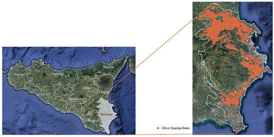
Figure 1.
Location of Syracuse province within Sicily (Italy).
Based on data availability, described in the following sections, the year 2000 was used for the simulation period, although the methodology could also be applied to different time series.
2.2. Input Data Acquisition and Processing
The VisTrails:SAHM requires data regarding the presence of the species in .csv format and other predictor layers in raster format (i.e., .tiff).
Citrus presence (Figure 1) data were obtained by overlaying the Sicilian Technical Regional Cartography (TRC) with the IT2000 orthophotos available in the Sicilian Land Information System (SITR). The orthophotos are derived from aerial acquisition, are geometrically corrected and are georeferenced within the ATA2000 project, which is commissioned by the Sicilian Region. The overlay was carried out by using GIS software (specifically, ArcGIS® for Desktop 10.3 and QGIS 3.10.0). In detail, about 10,000 georeferenced presence points were used as input data in the VisTrails:SAHM.
By using the GIS tools, 19 bioclimatic variables (Table 1) provided by the WorldClim database for three decades, from 1970 to 2000, were represented in raster format. WorldClim data are routinely used for cropland suitability studies because they provide a comprehensive picture of monthly, quarterly and annual bioclimatic conditions [12].

Table 1.
Explanation of the WorldClim bioclimatic variables.
Furthermore, the set of covariates was enriched by the Digital Terrain Model (DTM), in metres, which brings valuable information about the effects of altitude on plant presence. This layer is related to a 20 m resolution and DTM_20 was the related predictor.
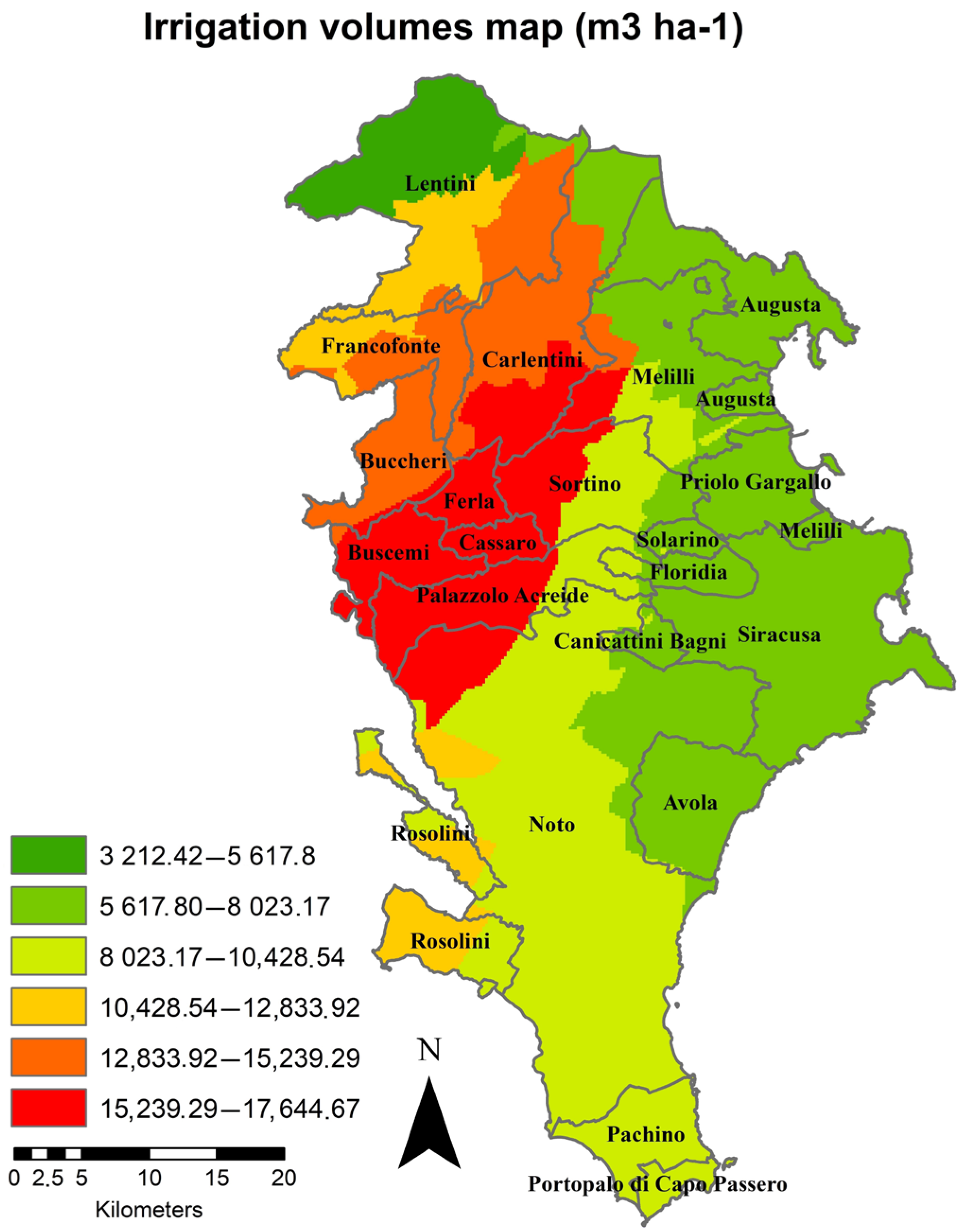
To simulate the effects of deficit irrigation, the watering volume was gradually reduced by 10% from the 100% values acquired from the A.C.Q.U.A project (‘Agrumicultura Consapevole della Qualità e Uso dell’Acqua’—‘Awareness of quality and use of water in Citrus cultivation’) [13], which surveyed the actual irrigation volumes in the area under study. These data can be acquired from the WebGIS of the project (http://www.distrettoagrumidisicilia.it/wp-content/web_gis/index.html, accessed on 5 January 2023). To transform irrigation data from point data to continuous data, the ‘Kriging Ordinary’ interpolation method was applied with default settings to the irrigation data to produce a map in raster format, hereafter named Sir_Irr (m3 ha−1), suitable for the models’ input (Figure 2).

Figure 2.
Irrigation volumes map with data from the A.C.Q.U.A. project.
2.3. Modules Selection
In the second phase of the methodology, the modules within VisTrails:SAHM were selected based on the scheme defined by Morisette et al. [14] (Figure 3). The scheme establishes which modules are suitable for each phase of the model in relation to problems of the type examined in this study. In addition to that scheme, the ApplyModel module was added to allow comparison among various simulations of increasing deficit irrigation.
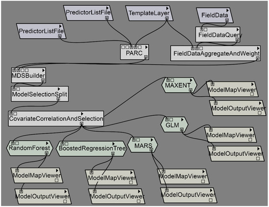
Figure 3.
VisTrails v.2.2.3 pipeline with the SAHM v.2.0.1 (Software for Assisted Habitat Modeling) for this specific study.
The most important software modules, at each stage, were the following:
- -
- in the ‘Preprocessing phase’, the key module to speed up the input processing phase was the PARC module, which allows for projection, aggregation, resampling and clipping of input geospatial data to match the TemplateLayer;
- -
- in the ‘Preliminary model analysis and decision’ phase, the ModelSelectionSplit and CovariateCorrelationAndSelection modules were used. The first module reserves some of the data from the model training process for testing the model and reports evaluation metrics on all models. Based on the literature in this field, the training ratio of 70% with a testing ratio equal to 30% for presence data was considered in this study. In fact, the amount of presence data proved to be critical for the prediction, and those ratios produced a more robust model [6,8,9].
Finally, the CovariateCorrelationSelector module provides a breakpoint in the modelling workflow to allow the user to evaluate how each variable explains the distribution of the sampled data points and allows the user to remove any variables that may be highly correlated with others [15]; in fact, collinearity can lead to large model prediction errors [6]. To select only predictors that were less strongly correlated, the maximum value between the Pearson, Spearman and Kendall coefficients calculated for the pairs of variables was used; specifically, the threshold value for the three coefficients was set to ±0.8 [4,16,17]. Therefore, since coefficient values higher than the thresholds infer that there is a strong association between the two variables, in this case one of the two variables was considered and the other was discarded.
The description of the influence of predictors in the model was analysed through the responseCurve graphs provided by the software for each model. They describe the values of each predictor in relation to the probability of presence in order to select the range where the probability is higher, and describe the contribution of the predictor to the probability for the specific model [18].
2.4. Accuracy Measures
In this study, the measurement of the accuracy of the SDM classifications was conducted through calculation of the Receiver Operating Characteristic (ROC) curve and the related metric Area Under the Curve (AUC), a threshold-independent metric that evaluates the ability of a model to discriminate the presence from the background [8,9].
For the interpretation of the values of the area under the ROC curve it is possible to refer to the classification reported in the study of D’Arrigo et al. [19]:
- (1)
- AUC = 0.5 the test is not informative;
- (2)
- 0.5 < AUC ≤ 0.7 the test is inaccurate;
- (3)
- 0.7 < AUC ≤ 0.9 the test is moderately accurate;
- (4)
- 0.9 < AUC < 1.0 the test is highly accurate;
- (5)
- AUC = 1 perfect test.
Moreover, ΔAUC values, computed as the difference between the AUC of the training and the AUC of the testing, were considered for assessing overfitting, according to Mukherjee et al. [20]. Specifically, when the ΔAUC value exceeds 0.05, overfitting occurs [3].
Moreover, True Skills Stat (TSS) [21] was considered in this study to compare the different models by applying the following relations (Equation (1)):
in which Sensitivity (Equation (2)) (or True Positive Rate—TPR) and Specificity (Equation (3)) (or True Negative Rate—TNR) are defined as:
where TP is the number of True Positives, FN is the number of false negatives, TN is the number of True Negatives, and FP is the number of False Positives.
TSS = Sensitivity + Specificity − 1
The thresholds for significance of these metrics are referred to as random rankings. These have on average an AUC value of 0.5, whereas a perfect ranking achieves the best possible AUC value equal to 1.0; models with values above 0.75 are considered potentially useful [22]. TSS ranges from −1 to +1, where +1 indicates perfect agreement and zero or negative values indicate a performance no better than random [19].In this study, according to some authors [23,24], the difference ΔTSS between training and testing was computed in order to analyse TSS.
To divide the continuous model predictions into binary presence/absence predictions, the maps were produced by using thresholds specifically computed by the software for each model [25].
Elaborations on output surfaces at a 10% step of probability (classes 1 to 10) were carried out by computing the weighted variation in percentage between the surface Supi related to the considered deficit irrigation level and the surface Sup100 related to 100% irrigation, according to the following relation (Equation (4)):
Moreover, other elaborations were carried out to relate the surface area of the class to the overall surface of the province.
3. Results and Discussion
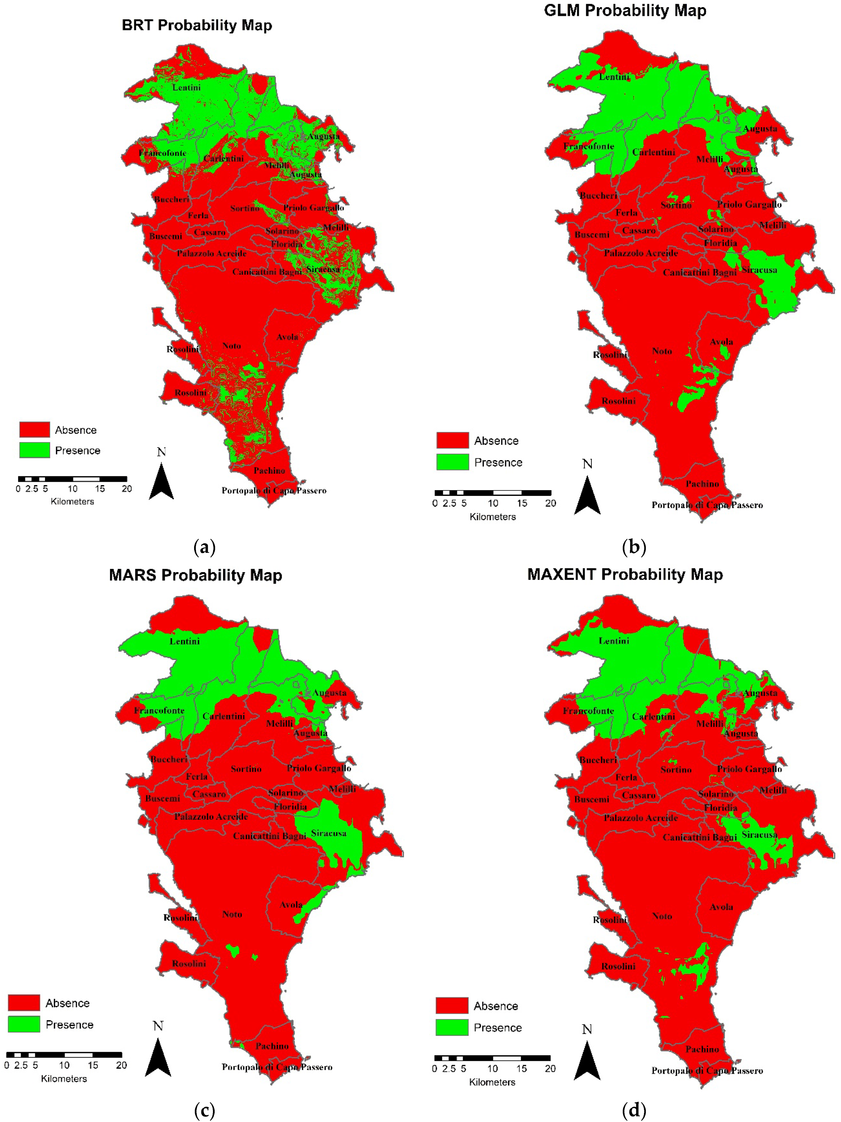
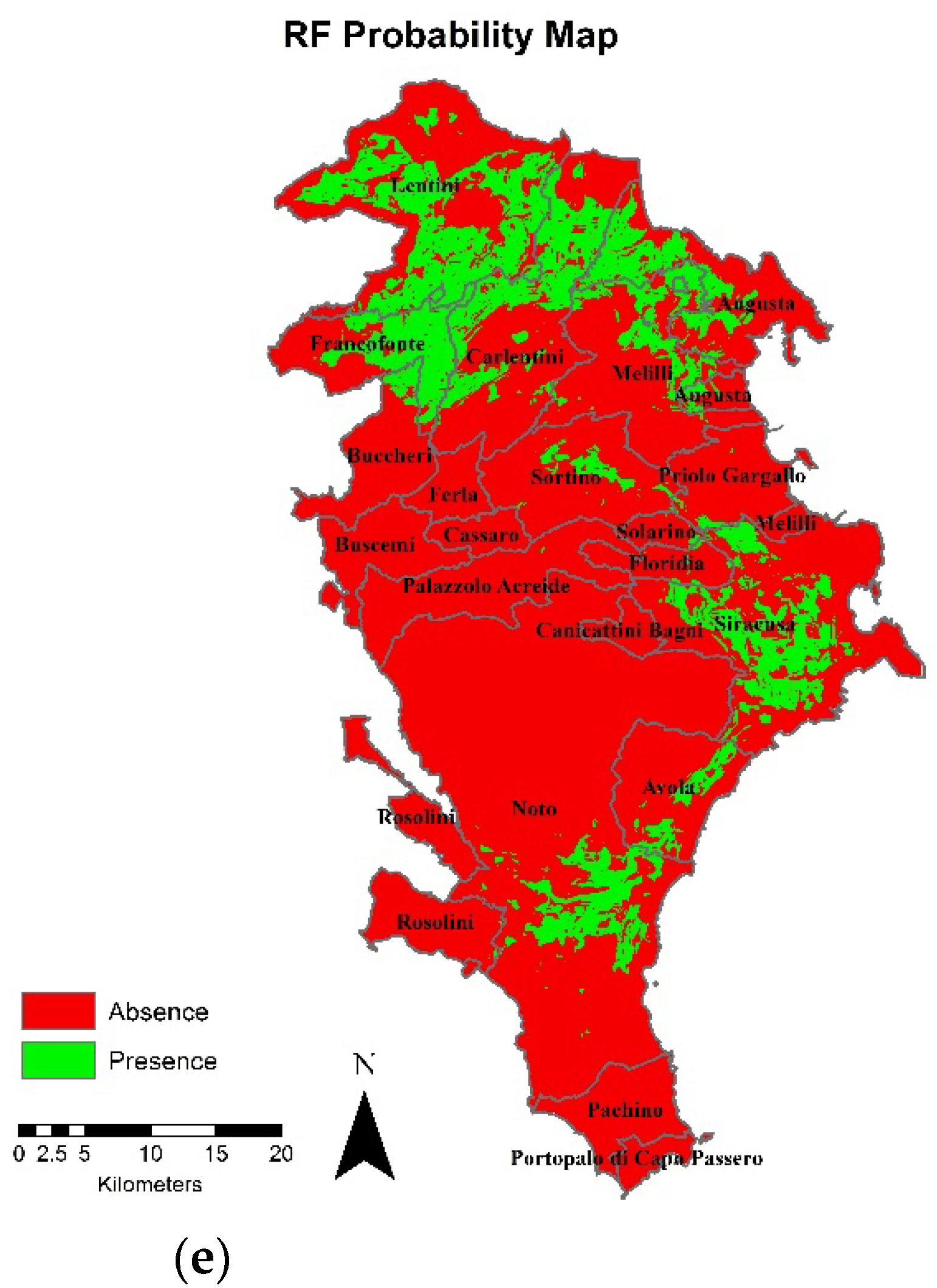
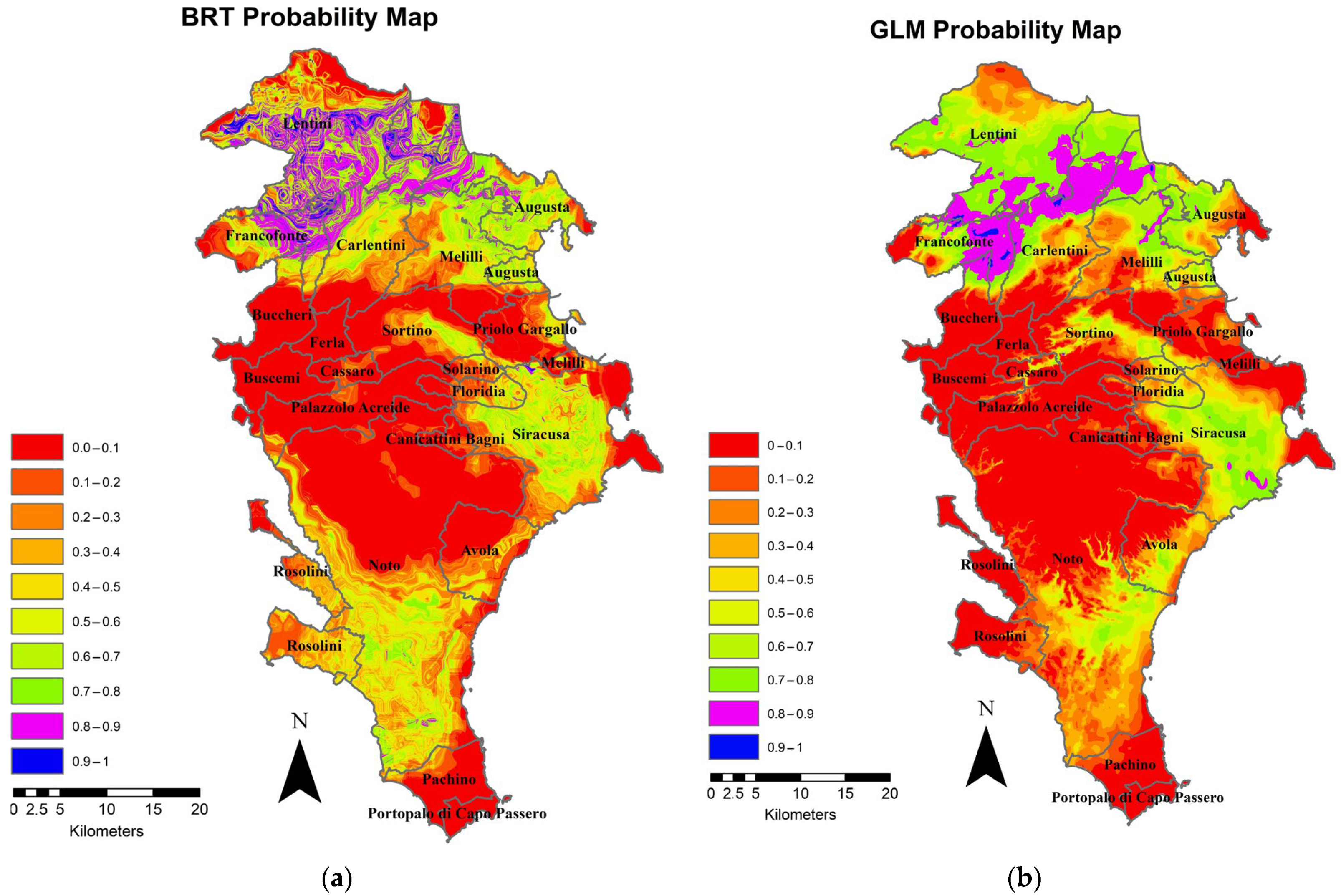
All models showed a quite stable output: there was wide consensus among the different models on the location of areas with the highest probability of presence for the species. Specifically, the results showed that the highest probability of presence of citrus trees in the study area was found in the northern areas of the province and in eastern ones (i.e., in the municipalities of Syracuse, Noto and Avola). The central and southern areas were considered unsuitable by all models (Figure 4). General results were consistent with data showing that reliable processes have been proposed.
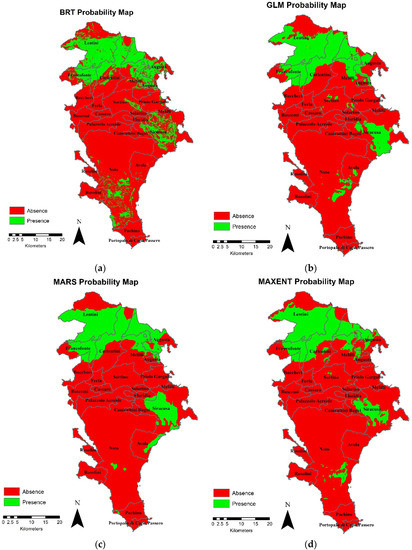

Figure 4.
Probability Maps, obtained by applying the threshold for probability for each model, in the province of Syracuse: (a) BRT; (b) GLM; (c) MARS; (d) MaxEnt; and (e) RF.
In Figure 4, according to Akpoti [18], the probability was subdivided into presence/absence through the utilisation of the threshold values computed by each SDM in order to allow comparisons among the different models’ outputs. The threshold values obtained for this case study were: 0.59 for RF; 0.55 for Mars; 0.4095 for MaxEnt; 0.61 for GLM; and 0.57 for BRT.
Based on these thresholds and the use of GIS tools, a detailed territorial analysis at the provincial level was carried out (Figure 4). Presence areas (in green colour) have a continuous aspect in GLM, MARS and MaxEnt models (Figure 4b–d), whereas in RF and BRT models (Figure 4a,e) those areas are composed of polygons with holes. The greatest differences among the models’ outputs were found in the northern part of the province (especially in the municipalities of Francofonte, Carlentini and Augusta) and in the inner part of the territory (municipalities of Sortino and Floridia), where, for instance, the MARS model showed no presence of the species.
The overall surface area (km2) where the models predict a probability of presence above the threshold (in green) are the following: 519.59 for BRT; 484.35 for GLM; 505.17 for MARS; 676.30 for MaxEnt; and 401.45 for RF. Therefore, the RF model underestimated most compared to the average value of the model predictions, whereas the MaxEnt model overestimated. The differences among the simulations of the presence areas obtained by the BRT, GLM and MARS models were not great (with a maximum of about 35 km2), and the information of the territorial distribution of probability of presence acquired by GIS representation was extremely valuable.
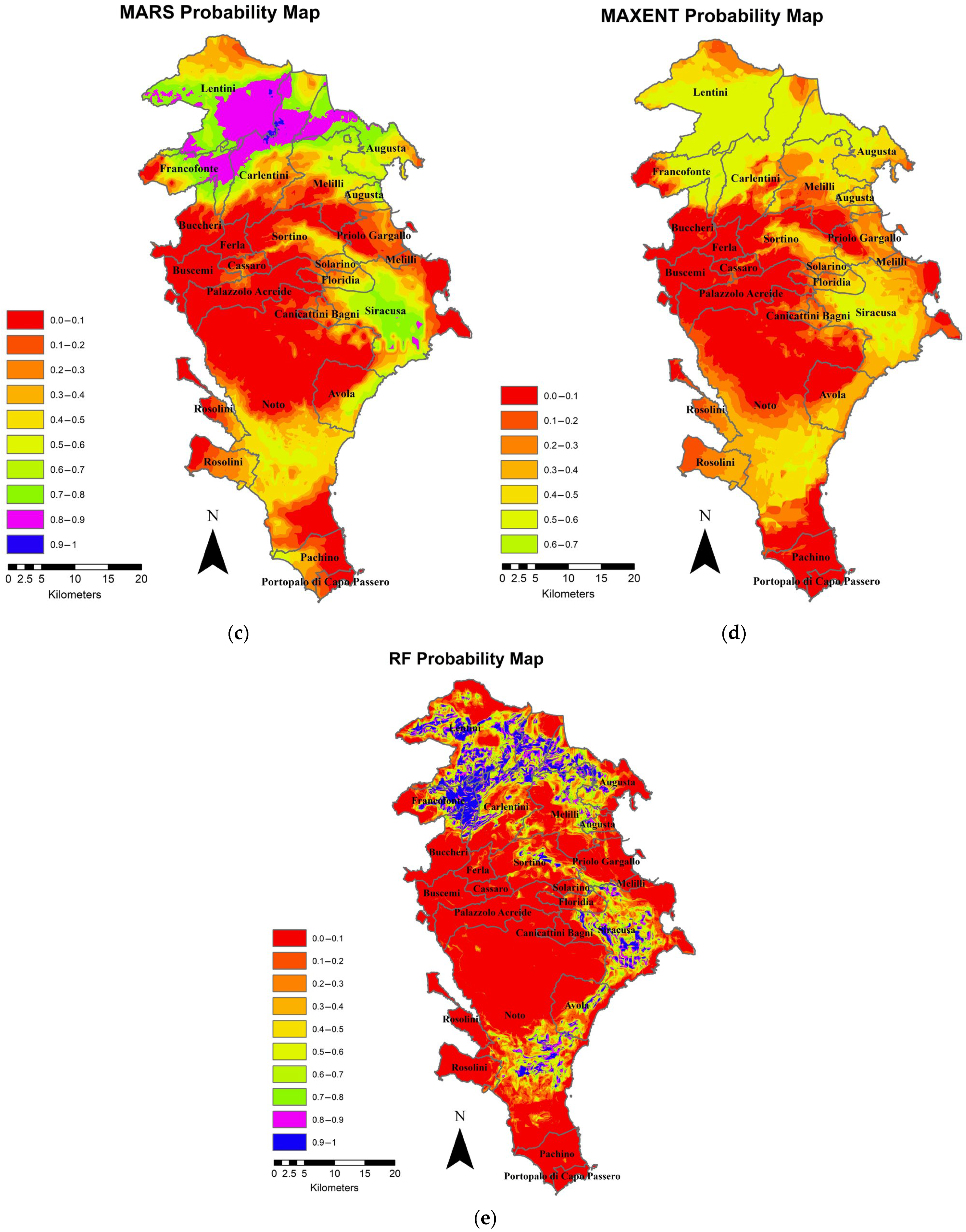
For a more in-depth spatial analysis of the results, the probability was subdivided into 10 classes, at 10% intervals of probability, in order to refine comparison among the different areas (Figure 5). The surfaces of each class were calculated for each model by using the QGIS software (Table 2). From the comparison of Class 10 obtained by the RF and BRT models, the localisation of the areas was similar (in the municipalities of Lentini, Augusta, Carlentini, Francofonte, Melilli, Sortino, Siracusa and Avola e Noto) and quite spread out, though the surfaces were wider in the RF model than in the BRT model. In the GLM model, Class 10 was found in a lower number of areas (in the municipalities of Francofonte and Lentini) and in even fewer for the MARS model (in Carlentini municipality). The greatest surface areas for Class 1 (1178.5 km2) and Class 10 (116.1 km2) were confirmed for the RF model.
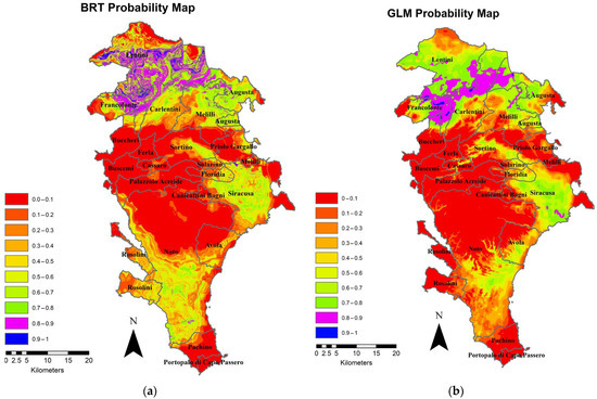

Figure 5.
Probability Maps, obtained by applying the 10-classes subdivision for probability, for each model in the province of Syracuse: (a) BRT; (b) GLM; (c) MARS; (d) MaxEnt; and (e) RF.
Table 2.
Values of the surface areas (km2) for each class and model: in bold green the presence data, while in red the absence data.
Moreover, the sum of the surfaces from Class 7 to Class 10 for each model that required summing the values from Class 5 to 10, except for the MaxEnt model, confirmed the outcomes obtained by the application of the thresholds, i.e., MaxEnt had the highest area (703.1 km2) whereas RF had the lowest one (393.3 km2). GLM was close to the mean value of the overall surface computed on all of the models’ outputs (496.46 km2) and BRT and MARS slightly overestimated the overall surface area (444.8 and 442.7 km2, respectively), whereas MaxEnt highly overestimated and RF moderately underestimated compared to the average value.
To assess which model had a higher capability to estimate the probability of the presence of citrus, the metrics produced by the SDM in VisTrails:SAHM were considered and analysed.
The analysis of the metrics for the classifications (Table 2 and Table 3) highlighted that the AUC of all the models exceeded 0.83; therefore, the classifications were assessed as ‘very good’, and the TSS was higher than 0.50.
Table 3.
Values of the metrics for training and testing and for each model.
Based on the results reported in Table 2, the BRT model had the highest metrics for training among the models whereas the MARS model showed the lowest metrics.
In Table 3, the BRT model shows a ΔAUC equal to 0.08, thus highlighting that model overfitting is high, and therefore this SDM was not considered as adequate. In detail, overfitting would make the algorithm produce very different predictions for similar data (low bias and high variance). The lowest ΔAUC equal to 0 was found for the RF model, while the values for MARS, GLM and MaxEnt showed a ΔAUC in the order of hundredths, thus also suitable because of the low overfitting associated.
Moreover, for ΔTSS, Table 4 shows that the BRT model had a high value (about 0.15) compared to those of the other SDMs, which had values in the range 0 ÷ 0.005.
Table 4.
Values of ΔAUC e ΔTSS for the different SDMs.
Based on all the considerations described above, RF can be considered the model with the highest ability to predict citrus coverage. Therefore, the subsequent simulations on deficit irrigation were carried out by applying the RF model.
Deficit Irrigation
To simulate the effects of deficit irrigation, the watering volume was gradually reduced by 10%, from 100% of the actual irrigation volume to 50%.
Based on the results of the elaborations, the probability maps showed that the increasing reduction of irrigation volume produced a reduction of the probability values of species presence, though the localisation of the areas was similar (Figure 6). Moreover, the greater the reduction of irrigation volume the greater the reduction of probability. The considerations derived from the maps are confirmed by the numerical data processed (Table 5 and Table 6).
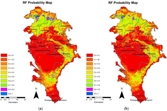
Figure 6.
Probability Maps for RF model, reporting a deficit irrigation of 80% (a) and 50% (b) of the actual value, in the province of Syracuse.
Table 5.
Values of the surface areas Si (km2) for the deficit irrigation from 100% to 50% of the actual value and the ten classes, for the RF model.
Table 6.
Values of the weighted difference in percentage Dsup, for the deficit irrigation from 100% to 50% of the actual value and the ten classes, for the RF model.
For RF, the sum of the surface areas from Class 7 to 10 proved that the deficit irrigation simulations would cause a maximum surface reduction of 173.41 km2 (at a deficit irrigation equal to 50% of the actual) and a minimum one of 75.99 km2 (at a deficit irrigation equal to 90% of the actual value) with an average value of 122.32 km2 (Table 5).
The reduction of irrigation would highly affect the probability of species presence, especially for Classes 9 and 10. For instance, for a 90% irrigation the surface of Class 10 would decrease by 85.36%(compared to 100% irrigation), and would decrease from 5.51% to 0.81% in relation to the whole surface of the province (Table 6 and Table 7). In contrast, for a deficit irrigation equal to 80% of the actual value, the surface area for Class 10 is 9.20 km2 (−92.07%) and 37.56 km2 (−64.82%) for Class 9 (Table 5 and Table 6). However, an increase of the surface of intermediate classes, mainly 6 and 7, would occur. For instance, the surface of Class 7 would increase by 65.29 km2 (mainly in the municipality of Lentini) compared to 100% irrigation, under the hypothesis of a reduction of irrigation to 60%.
Table 7.
Values of the ratio between the surface areas Si and the total area of the province Stot for the deficit irrigation from 100% to 50% of the actual value and the ten classes, for the RF model.
Although the loss of probability in one class could be compensated by the area in a lower class (albeit always considering the Classes 7 to 10, that have a higher probability than about 0.6, according to the thresholds of presence/absence), the surface loss would range from 19.3% (at 90% deficit irrigation) to 44.09% (at 50% deficit irrigation).
In Table 6, the weighted variation in percentage between the deficit irrigation level and the 100% irrigation was reported; Dsup shows that the probability of presence drastically reduced for Classes 8 to 10 during increased irrigation reduction in the territory. This is confirmed in the probability maps, where as the irrigation contribution decreases there is a progressive reduction in the extent of the presence of the species in the areas until the presence remains only in the north and east of the provincial territory.
Therefore, the spatial analysis outcomes show that eastern and northern areas of the province would be the most suitable for deficit irrigation for this kind of species, whereas for the southern citrus producing areas of the province it would not be advisable to perform deficit irrigation.
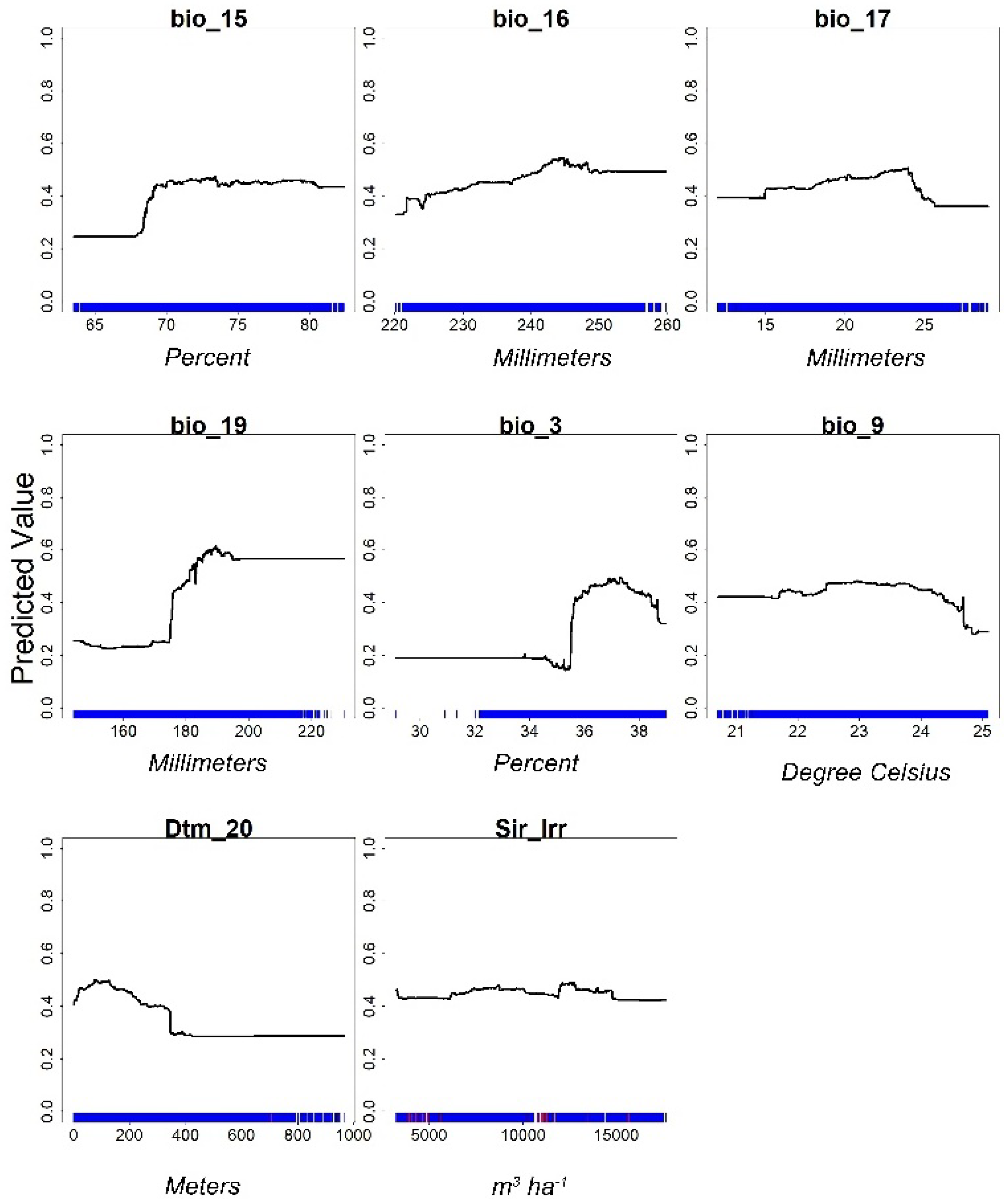
The analysis of the ResponseCurve produced for the RF model (Figure 7) provided useful information about the range of the predictors that most contribute to the probability values.
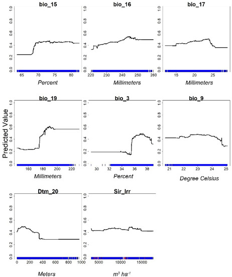
Figure 7.
ResponseCurves of the predictors for the RF model, for the case study analysed.
The predictors Bio_15 (Precipitation Seasonality (Coefficient of Variation)), Bio_16 (Precipitation of Wettest Quarter), Bio_19 (Precipitation of Coldest Quarter), Bio_9 (Mean Temperature of Driest Quarter), Bio_17 (Precipitation of Driest Quarter), Bio_3 (Isothermality), DTM_20 and Sir_Irr were considered by the models as those affecting the probability of the presence of citrus in the case study analysed.
The analysis of the ResponseCurve graphs produced valuable information on each predictor range associated with the fitted values while holding all other predictors constant at their means. These graphs can be studied to assess whether the relationships agree with the biological meaning of the species under study [15].
Specifically, the graph for DTM_20 showed that the altitudes suitable for citrus production were correctly identified by the RF model, i.e., points with a probability greater than the threshold were found for altitudes lower than 400 m a.s.l. [26,27]. The response curves of predictors showed the following ranges where the predicted value for the probability of citrus presence is higher: Bio_3 between 35% and 39%, showing the diurnal temperature range lower than annual one; Bio_19 greater than 180 mm, representing the level of overall precipitation during the coldest quarter of the year; Bio_15 greater than 70%, showing the variation of monthly precipitation during the year; Bio_16 above 220 mm of rain, showing the precipitation amount in the wettest quarter; Bio_17 above 15 mm, indicating the minimum precipitation of the driest quarter. The contribution to prediction, equal to about 0.45, deriving from the values of Sir_Irr confirms the importance of water input for the citrus crop; in fact, most of the influential bioclimatic variables are related to precipitation.
It is well known, in fact, that citrus trees require large volumes of water compared to other tree crops, especially when precipitation scarcity is recurrent, and require suitable temperature levels and other growing conditions beneficial for achieving high quality productions. Therefore, water consumption is one of the most demanding issues for the citrus sector, especially in times of climate variability and change.
4. Conclusions
The research study described in this paper investigated the feasibility of applying algorithms for SDMs to predict citrus distribution in a territory in order to derive information on SDM application in the Mediterranean climate and analyse the main factors that influence the presence of the citrus plant. The aim of providing improved knowledge on spatial distribution of the species was also achieved by analysing the effects of deficit irrigation in the case study of the province of Syracuse, Italy.
This study represents the first step toward an in-depth spatial knowledge of citrus in Mediterranean areas in relation to bioclimatic variables and other driving factors. Climate covariates and terrain elevation as well as irrigation were analysed in this study as major predictors suitable for this knowledge. General uniformities in the models’ predictions suggest that the multi-model approach contributes to an increased consistency of outcomes. Modeling showed that the BRT and RF models produced higher evaluation metrics compared to the other models; however, the BRT model suffered from overfitting. GIS contributed to the analysis of the outcomes by showing and quantifying the spatial distribution of citrus presence as well as by allowing comparison among the simulations of different levels of irrigation.
This study was limited to the analysis of outcomes related to the default settings of the models’ parameters. Investigation on model parameters is the object of on-going studies aimed at fine-tuning the performance of the predictions, and research is in progress to investigate input data by involving computation of the bioclimatic data from local weather stations. Further analysis could consider predictions of future probability of species presence based on climate models for the determination of future bioclimatic predictors.
Author Contributions
Conceptualization, C.A. and G.A.C.; methodology, C.A. and G.A.C.; software, G.A.C.; validation, P.R.D. and C.A.; formal analysis, P.R.D. and F.M.; investigation, P.R.D. and C.A.; resources, C.A.; data curation, G.A.C. and F.M.; writing—original draft preparation, C.A. and G.A.C.; writing—review and editing, C.A., F.M. and P.R.D.; visualization, P.R.D.; supervision, C.A.; project administration, C.A.; funding acquisition, C.A. All authors have read and agreed to the published version of the manuscript.
Funding
The research study was funded by the University of Catania through the project ‘PON “RICERCA E INNOVAZIONE” 2014–2020, Azione II—Obiettivo Specifico 1b—Progetto “Miglioramento delle produzioni agroalimentari mediterranee in condizioni di carenza di risorse idriche—WATER4AGRIFOOD”, Cod. progetto: ARS01_00825, CUP: B64I20000160005 and it is in line with ‘Piano incentivi per la ricerca di Ateneo 2020–2022-Linea 2’ project on ‘Engineering solutions for sustainable development of agricultural buildings and land—LANDSUS’ (ID: 5A722192152) coordinated by Claudia Arcidiacono.
Data Availability Statement
Data available upon request.
Acknowledgments
The authors wish to thank the Sicilian Region for SITR data (https://www.sitr.regione.sicilia.it/ accessed on 13 June 2022).
Conflicts of Interest
The authors declare no conflict of interest.
References
- Del Bravo, F.; Finizia, A.; Lo Moriello, M.S.; Ronga, M. La Competitività Della Filiera Agrumicola in Italia; Rete Rurale Nazionale 2014–2020; ISMEA: Rome, Italy, 2020. [Google Scholar]
- Verner, D.; Tréguer, D.; Redwood, J.; Christensen, J.; Mcdonnell, R.; Elbert, C.; Konishi, Y.; Belghazi, S. Climate Variability, Drought, and Drought Management in Morocco’s Agricultural Sector—World Bank Report 2017. Available online: https://openknowledge.worldbank.org/bitstream/handle/10986/30603/130404-WP-P159851-Morocco-WEB.pdf (accessed on 23 November 2022).
- Olonova, M.V.; Vysokikh, T.S.; Mezina, N.S. Structure of Ecologo-Climatic Niches of Poa palustris L. and P. nemoralis L. (Poaceae) in Asian Russia. Contemp. Probl. Ecol. 2018, 11, 604–613. [Google Scholar] [CrossRef]
- Leanza, P.M.; Valenti, F.; D’Urso, P.R.; Arcidiacono, C. A combined MaxEnt and GIS-based methodology to estimate cactus pear biomass distribution: Application to an area of southern Italy. Biofuels. Bioprod. Biorefining 2022, 16, 54–67. [Google Scholar] [CrossRef]
- West, A.M.; Jarnevich, C.S.; Young, N.E.; Fuller, P.L. Evaluating Potential Distribution of High-Risk Aquatic Invasive Species in the Water Garden and Aquarium Trade at a Global Scale Based on Current Established Populations. Risk Anal. 2019, 39, 1169–1191. [Google Scholar] [CrossRef] [PubMed]
- Piekielek, N.B.; Hansen, A.J.; Chang, T. Using custom scientific workflow software and GIS to inform protected area climate adaptation planning in the Greater Yellowstone Ecosystem. Ecol. Inform. 2015, 30, 40–48. [Google Scholar] [CrossRef]
- Diniz-Filho, J.A.F.; Mauricio Bini, L.; Fernando Rangel, T.; Loyola, R.D.; Hof, C.; Nogués-Bravo, D.; Araújo, M.B. Partitioning and mapping uncertainties in ensembles of forecasts of species turnover under climate change. Ecography 2009, 32, 897–906. [Google Scholar] [CrossRef]
- West, A.M.; Evangelista, P.H.; Jarnevich, C.S.; Young, N.E.; Stohlgren, T.J.; Talbert, C.; Talbert, M.; Morisette, J.; Anderson, R. Integrating Remote Sensing with Species Distribution Models, Mapping Tamarisk Invasions Using the Software for Assisted Habitat Modeling (SAHM). J. Vis. Exp. 2016, 116, e54578. [Google Scholar] [CrossRef]
- West, A.M.; Kumar, S.; Brown, C.S.; Stohlgren, T.J.; Bromberg, J. Field validation of an invasive species Maxent model. Ecol. Inform. 2019, 36, 126–134. [Google Scholar] [CrossRef]
- Freire, J.; Silva, C.T.; Callahan, S.P.; Santos, E.; Scheidegger, C.E.; Vo, H.T. Managing Rapidly-Evolving Scientific Workflows. In Provenance and Annotation of Data; Lecture Notes in Computer, Science; Moreau, L., Foster, I., Eds.; IPAW 2006: Chicago, IL, USA; Springer: Berlin/Heidelberg, Germany, 2006; Volume 4145. [Google Scholar] [CrossRef]
- Pavone, P.; Spampinato, G.; Costa, R.; Minissale, P.; Ronsisvalle, F.; Sciandrello, S.; Tomaselli, V. La Vegetazione Forestale dei Monti Iblei (Sicilia Sud-Orientale): I Querceti. In Proceedings of the third national silviculture congress, Taormina, Sicily, Italy, 16–19 October 2009; Volume 1, pp. 234–239. [Google Scholar] [CrossRef]
- Fitzgibbon, A.; Pisut, D.; Fleisher, D. Evaluation of Maximum Entropy (Maxent) Machine Learning Model to Assess Relationships between Climate and Corn Suitability. Land 2022, 11, 1382. [Google Scholar] [CrossRef]
- Università Degli Studi di Catania; CREA; Distretto Agrumi Sicilia; CocoCola Foundation; A.C.Q.U.A. Project Results. 2020. Available online: https://www.distrettoagrumidisicilia.it/wp-content/uploads/Dossier-Acqua5.pdf (accessed on 6 September 2022).
- Morisette, J.T.; Jarnevich, C.S.; Holcombe, T.R.; Talbert, C.B.; Ignizio, D.; Talbert, M.K.; Silva, C.; Koop, D.; Swanson, A.; Young, N.E. VisTrails SAHM: Visualization and workflow management for species habitat modeling. Ecography 2013, 36, 129–135. [Google Scholar] [CrossRef]
- Talbert, C.; Talbert, M. User Documentation for the Software for Assisted Habitat Modeling (SAHM) Package in VisTrails; USGS (U.S. Geological Survey): Reston, VA, USA, 2001. [Google Scholar]
- Yang, X.Q.; Kushwaha, S.P.S.; Saran, S.; Xu, J.; Roy, P.S. Maxent modeling for predicting the potential distribution of medicinal plant, Justicia adhatoda L. in Lesser Himalayan foothills. Ecol. Eng. 2013, 51, 83–87. [Google Scholar] [CrossRef]
- Yi, Y.J.; Cheng, X.; Yang, Z.F.; Zhang, S.H. Maxent modeling for predicting the potential distribution of endangered medicinal plant (H. riparia Lour) in Yunnan, China. Ecol. Eng. 2016, 92, 260–269. [Google Scholar] [CrossRef]
- Akpoti, K.; Kabo-bah, A.T.; Dossou-Yovo, E.R.; Groen, T.A.; Zwart, S.J. Mapping suitability for rice production in inland valley landscapes in Benin and Togo using environmental niche modeling. Sci. Total Environ. 2020, 709, 136165. [Google Scholar] [CrossRef]
- D’Arrigo, G.; Provenzano, F.; Torino, C.; Zoccali, C.; Tripepi, G. I test diagnostici e l’analisi della curva ROC. G Ital. Nefrol. 2011, 28, 642–647. [Google Scholar]
- Mukherjee, T.; Sharma, V.; Sharma, L.K.; Thakur, M.; Joshi, B.D.; Sharief, A.; Thapa, A.; Dutta, R.; Dolker, S.; Tripathy, B.; et al. Landscape-level habitat management plan through geometric reserve design for critically endangered Hangul (Cervus hanglu hanglu). Sci. Total Environ. 2021, 777, 146031. [Google Scholar] [CrossRef]
- Allouche, O.; Tsoar, A.; Kadmon, R. Assessing the accuracy of species distribution models: Prevalence, kappa and the true skill statistic (TSS). J. Appl. Ecol. 2006, 43, 1223–1232. [Google Scholar] [CrossRef]
- Phillips, S.J.; Dudík, M. Modeling of species distributions with Maxent: New extensions and a comprehensive evaluation. Ecography 2008, 31, 161–175. [Google Scholar] [CrossRef]
- Baer, K.C.; Gray, A.N. Biotic predictors improve species distribution models for invasive plants in Western US Forests at high but not low spatial resolutions. For. Ecol. Manag. 2022, 518, 120249. [Google Scholar] [CrossRef]
- Brun, P.; Kiørboe, T.; Licandro, P.; Payne, M.R. The predictive skill of species distribution models for plankton in a changing climate. Glob. Chang. Biol. 2016, 22, 3170–3181. [Google Scholar] [CrossRef]
- Brun, P.; Payne, M.R.; Kiørboe, T. Trait biogeography of marine copepods—An analysis across scales. Ecol. Lett. 2016, 19, 1403–1413. [Google Scholar] [CrossRef]
- Pignatti, S. “Flora d’Italia”, 2017–2019 Citrus limon (L.). Burm. Fil. 2019, 2, 1090. [Google Scholar]
- Pignatti, S. La Flora d’Italia. Edagricole 1982, 2, 54. [Google Scholar]


Disclaimer/Publisher’s Note: The statements, opinions and data contained in all publications are solely those of the individual author(s) and contributor(s) and not of MDPI and/or the editor(s). MDPI and/or the editor(s) disclaim responsibility for any injury to people or property resulting from any ideas, methods, instructions or products referred to in the content. |
© 2023 by the authors. Licensee MDPI, Basel, Switzerland. This article is an open access article distributed under the terms and conditions of the Creative Commons Attribution (CC BY) license (https://creativecommons.org/licenses/by/4.0/).