Article

Improving Deep Learning Classifiers Performance via Preprocessing and Class Imbalance Approaches in a Plant Disease Detection Pipeline

Department of Biological and Agricultural Engineering, Texas A&M AgriLife Research, Texas A&M University System, Dallas, TX 75252, USA
*
Author to whom correspondence should be addressed.
Agronomy 2023, 13(3), 887; https://doi.org/10.3390/agronomy13030887
Submission received: 24 January 2023 / Revised: 10 March 2023 / Accepted: 14 March 2023 / Published: 16 March 2023
(This article belongs to the Section Precision and Digital Agriculture)

Abstract

:
The foundation of effectively predicting plant disease in the early stage using deep learning algorithms is ideal for addressing food insecurity, inevitably drawing researchers and agricultural specialists to contribute to its effectiveness. The input preprocessor, abnormalities of the data (i.e., incomplete and nonexistent features, class imbalance), classifier, and decision explanation are typical components of a plant disease detection pipeline based on deep learning that accepts an image as input and outputs a diagnosis. Data sets related to plant diseases frequently display a magnitude imbalance due to the scarcity of disease outbreaks in real field conditions. This study examines the effects of several preprocessing methods and class imbalance approaches and deep learning classifiers steps in the pipeline for detecting plant diseases on our data set. We notably want to evaluate if additional preprocessing and effective handling of data inconsistencies in the plant disease pipeline may considerably assist deep learning classifiers. The evaluation’s findings indicate that contrast limited adaptive histogram equalization (CLAHE) combined with image sharpening and generative adversarial networks (GANs)-based approach for resampling performed the best among the preprocessing and resampling techniques, with an average classification accuracy of 97.69% and an average F1-score of 97.62% when fed through a ResNet-50 as the deep learning classifier. Lastly, this study provides a general workflow of a disease detection system that allows each component to be individually focused on depending on necessity.

1. Introduction

Food security has emerged as one of many pressing challenges due to the population’s rapid growth and the gradually declining amount and quality of arable land [1,2]. With the advent of advanced technologies, controlled environment agriculture (CEA) has progressively come to represent the growth of modern agriculture because it not only makes optimal use of the land but also allows for the year-round cultivation of some crops, such as vegetables [3]. Greenhouses have been demonstrated to be effective environments for the growth and development of crops, making them one of the key products of CEA production.
A range of nutrients the body needs can be found in vegetables, one of the essential foods for a person’s daily diet. Despite the advantages, the spread of vegetable pests and diseases can quickly result in a sharp decline in food production [4]. The threat of disease spread in CEA is more serious due to favorable conditions such as high temperature and humidity. Thus, the early detection of vegetable disease is critical to increasing agricultural productivity in a sustainable way. Due to their high rate of error, time-consuming process, and low precision, traditional disease recognition techniques are no longer enough for contemporary agricultural production. The deep-learning-based image recognition of vegetable diseases is demonstrated with a variety of vegetable diseases, including tomato early blight, tomato late blight, tomato yellow leaf curl, tomato septoria leaf spot, and tomato target spot, among others, with high accuracy that is better than traditional methods and manual diagnosis [5,6]. As a result, it has become urgently necessary and a development trend in CEA to offer ways to enhance deep learning for disease detection through various technological means.
Bacterial wilt (Ralstonia solanacearum) of tomato, one of the main bacterial agents of bacteria disease, is responsible for a sizable amount of the disease burden [7]. It is one of the most devastating bacterial agents that affects more than 200 plant species. Bacterial wilt pathogen enters through microscopic injuries (frequently caused by insects) during cultivation or transplanting of tomato plants under favorable disease conditions and clogs the vascular tissue within the stem, preventing water and nutrients from circulating throughout the plant, showing wilting of the leaves. Therefore, early detection of tomato bacterial wilt disease is critical to be able to apply precise pesticide treatment. To the best of our knowledge, this is the first work to address bacterial wilt disease detection, as it differs from other surveyed vegetable diseases in terms of its symptoms.
For the detection of plant leaf diseases, digital signal processing and computer vision processes have recently grown in popularity. These methods go through several steps, including image preprocessing, segmentation, feature extraction, and classification of disease class, which is a workflow to follow in typical object detection. Convolutional neural networks (CNN), a widely used deep learning model, successfully analyzes visual images and can readily separate the necessary characteristics with its multi-layered structure. CNN can easily detect and classify objects with minimal preprocessing. We introduce the workflow for our plant disease detection, which is illustrated in Figure 1.
To further explain, we begin by preprocessing the input so that the effect of noise, which is frequently ignored, can be minimized. The preprocessing phase is important for enhancement of the image before providing the image to the classification model. A lot of noise, particularly poor background contrast, can be present in images taken by sensors and cameras during image acquisition, which has an impact on the segmentation accuracy. As seen in Unay et al. [8], the preprocessing phase involves a variety of procedures, such as image enhancement and color space transformation. For instance, image preprocessing techniques can be used to blacken the shorter sides of the images so that they become the same proportion, preventing image distortion while preserving the original images’ content. Researchers have carried out some studies on image preprocessing techniques for various agricultural applications, such as the study of Gavhale et al. [9], where the authors presented a system for the unaffected region of plant leaves based on image preprocessing techniques. The study’s recommended method improved the effectiveness of the color images, which finally aided in the extraction of diseases with greater efficiency. Additionally, Vetal and Khule [10] provided four diseases of tomato for classification, where the image preprocessing techniques are applied before multi-class SVM model was used for classification. However, they did not thoroughly explore the potential of preprocessing or examine how various strategies might be applied to images.
On the other hand, it is possible to think of the task of identifying diseases from image data as one of visual anomaly detection. The process of distinguishing or categorizing odd observations from data is known as anomaly detection. The data sets available for anomalous events and anomaly detection are inevitably skewed due to the rarity of anomalous events. Data sets related to plant diseases are not an exception and frequently display a magnitude imbalance.
Researchers have mostly employed two types of methods to enhance the classification accuracy of unbalanced data sets. An algorithmic method and a data-level approach to the problem are two different ways to tackle it. The original data are left intact in the first method. The classifier, however, has been altered at the algorithmic stage to skew against the minority class. Cost-sensitive learning [11] and recognition-based learning [12] are two examples. Cost-sensitive learning places a high emphasis on the costs associated with various forms of misclassification. This learning method seeks to keep overall costs minimal [13]. To add or remove samples at the data level and create a balanced data distribution, sampling or synthesizing processes are used [14]. In this study, the data-level approaches are of particular interest.
Utilizing sampling techniques—oversampling or undersampling—is a common strategy for addressing data imbalance. Undersampling eliminates samples from the majority class from the data set, whereas oversampling adds duplicates of selected minority class samples at random. Although oversampling has been demonstrated to be a reliable and successful method [15], balance is only possible at the expense of an elevated risk of overfitting [16]. A variation of random oversampling that duplicates random images while applying obfuscating alterations, such as rotation, blur, cropping, contrast, sharpening, translation, etc., is also applicable to image data sets. This method has been employed for some time in various applications, such as the recognition of human diseases [17] and the classification of plant leaves [18].
Additionally, generative adversarial networks (GANs) and their derivatives have been used to create new samples on diverse image data sets to enhance the adaptability of training images [19]. The addition of the GAN network was quite useful in enhancing the variety and diversity of training images, which helped to contribute to high detection performance, as emphasized in Mai et al. [20] and Hu et al. [21]. To create more synthetically diseased images and create a balanced data set, some GAN variations have been suggested to transform images of healthy plants to diseased images [22]. In order to improve network generalizability and avoid the overfitting issue, a data augmentation method for tomato disease detection used the conditional generative adversarial network (C-GAN) [23] to produce synthetic images of tomato plants. To train their apple lesion detection system, more data on diseased apples was generated using a GAN variation termed CycleGAN [24]. However, CycleGAN lacks explicit attention methods for transforming specific objects in images, which makes it limited in producing high quality images. As a result, the generated images might not have significant impact on the robustness of the model used to diagnose plant diseases [25]. As a data augmentation tool to enhance the performance of plant disease diagnosis, LeafGAN is another GAN-based method based on image-to-image translation that produces diseased images via transformation from healthy images [25]. By converting healthy leaf data into leaf data for numerous diseases, it aims to balance the data set and produce clear visuals. In this work, we choose a noise-to-image translation strategy, where DCGAN has been the most popular method.
Except for a few studies where simplicity is frequently sacrificed in favor of performance, the attention on correcting the underlying class imbalance and overall lack of samples is largely overlooked. In addition, there is a dearth of work contrasting the more modern GAN-based strategies with the conventional sampling-based techniques for the problem of identifying image-based plant diseases. Furthermore, these existing systems are not directly comparable to one another due to variations in the experimental environments and the data sets on which they were trained. In contrast to the augmentation techniques mentioned above, in this study, we apply three techniques SMOTE [16], M2m [26] and DCGAN [27] to deal with an imbalanced data set in plant disease detection. Most deep learning research for plant disease detection largely ignores various preprocessing strategies for disease detection and classification; however, this work also included an in-depth analysis of them.
In this paper, we emphasized the approach’s simplicity while weighing its broad applicability and ease of implementation against its performance. The significance of this article can be summarized as follows:
  • To increase the pertinent features in the plant leaf, we conduct a qualitative and quantitative evaluation of a variety of image pre-processing approaches (described in Section 2.1. We discovered that contrast limited adaptive histogram equalization (CLAHE), in conjunction with image sharpening, can give a deep classifier a notable significant improvement.
  • We examine the effectiveness of data balancing approaches across many categories, focusing on how adding new synthetic data affects the classifier’s ability to learn. With the use of three data augmentation techniques—synthetic minority oversampling technique (SMOTE), generative adversarial networks (GAN), and major-to-minor translation (M2m)—we conducted extensive tests on the data set.
  • We investigate the detection of bacterial wilt disease on tomato plants, which is unique due to its symptoms.
The rest of this paper is organized as follows: Section 2 features the methodology of the research work. In Section 3, we present the experimental protocol, as well as the qualitative and quantitative analysis of the findings, and lastly, Section 4 concludes the paper with some final remarks.

2. Materials and Methods

2.1. Image Preprocessing Techniques

High-resolution (HR) images enable better prediction judgments to be made from raw images. In many cases, a higher-resolution image than a low-resolution image will allow for better prediction of plant diseases. HR images make it possible to create computerized diagnostic systems to help farmers spot problems early and make informed decisions. Additionally, it allows for more accurate object detection and image segmentation. High-pass filters are a straightforward example of a non-learning based deterministic image preprocessing method; however, they struggle to keep the enhancement level on a larger range of images when there is significant variation. Making these techniques input-adaptive is one way to improve these techniques. This might be incredibly successful when used to raw images, where great unpredictability is typical.

2.1.1. Adaptive Histogram Equalization (AHE)

AHE is a technique for improving the contrast of images that only affects a tiny portion of the image (i.e., tile) [28]. As an improvement to histogram equalization, the contrast transform function for each tile is calculated and applied for the tile to boost contrast (HE). Additionally, this approach has poor adaptive contrast when there are sections of the image that are darker or brighter than most of the image [28]. Given that different portions of an image’s contrast are likely to differ, this could be useful for plant images. However, using the AHE method increases the contrast in near-constant sections of the image as well as causes augmented noise in these sections.

2.1.2. Contrast Limited Adaptive Histogram Equalization (CLAHE)

This is a method for resolving the drawbacks of AHE. It improves image contrast and uniformly equalizes intensities by lowering the noise amplification of the tiles with an adjustable grid size and contrast-limiting clip threshold [29]. The CLAHE limits the augmentation by clipping the histogram at a predefined amount before computing the cumulative distribution function (CDF). Compared to AHE, CLAHE performs better even though noise is not entirely eliminated. Grid size and clip limit serve as the parameters that define the CLAHE. These two factors mostly determine improved image quality. Because the input image has a very low intensity and a greater clip limit flattens its histogram, the image gets brighter when the clip limit is increased. The dynamic range widens, and the visual contrast rises as the grid size rises. When employing image entropy, the two parameters chosen at the location of maximum entropy curvature result in subjectively high-quality images.

2.1.3. Image Sharpening (SH)

By enhancing the contrast of edges in images, sharpening is one of the fundamental procedures used to boost the visual impression of images. To sharpen an image, a sharpening mask is first acquired by running the image through a high-pass filter, which increases the high-frequency components of the image. After the sharpening operation, the gradient of the edge will increase. Although little irregularities are seen in images are highlighted, the increase in noise in the image is undoubtedly a factor.

2.1.4. CLAHE + Sharpening (CL + SH)

A combination strategy such as CLAHE + Sharpening (CL + SH), which applies CLAHE first and then performs an image sharpening phase, is effective. Two factors served as the driving forces behind this composite image preprocessing technique. First, CLAHE improves an image without being affected by noise by using a clip limit; however, this also limits CLAHE’s ability to improve images, leaving room for future advancements. Second, noise compromises image sharpening even when it results in an unconstrained comprehensive improvement. As a result, the serial use of these two methods may enable CLAHE to enhance and reduce noise in the image. Then, in the following phase, sharpening might further improve the image’s quality without causing distortion.

2.2. Addressing Class Imbalance

Class imbalance problems play a major factor in object detection by having adverse effects on the final detection performance. The level of imbalance in a training set can be assessed using the imbalance ratio (IR), which is the proportion of the number of members from the largest class to those from the smallest class. This typical phenomenon hinders numerous applications in medical diagnosis and plant disease detection. As a result, the minority class(es), frequently the more significant class, often results in misclassification. Class imbalance happens when one class is over-represented. Foreground–foreground imbalance, where a limited number of classes frequently predominate the data set, or foreground–background imbalance, where the background instances considerably outweigh the positive ones, are two possible manifestations of this problem.
A significant portion of minority class representatives is regularized due to the dearth of minority class representatives. As a result, there is a bias in favor of placing new points into the class with the majority. There are several approaches to protect the classifier from class imbalance. Due to their widespread use and significance, we will concentrate on just three of these techniques in this article. We deliberately refrain from looking into the effectiveness of undersampling to mitigate the impact of class imbalance. Numerous studies have criticized undersampling as ineffective because it causes the loss of crucial majority class points, which causes information to be lost that is detrimental to deep learning models [30,31,32].
On the other hand, oversampling increases the number of samples from underrepresented classes and has been demonstrated to be a successful and reliable approach [15]. However, it can suffer from over-fitting when performed carelessly because bias is introduced by duplicating samples from underrepresented classes [31,33]. These approaches discussed above (undersampling and oversampling) are commonly referred to as resampling the data set, and the research mentioned above is only concerned with foreground-foreground class imbalance (i.e., there is no background class).

2.2.1. Synthetic Minority Oversampling Technique (SMOTE)

SMOTE, a popular oversampling method, is a technique for enhancing learning from imbalanced data by interpolating new samples from neighboring samples [16]. It produces a new point from the convex combination of a pair of neighboring minority class instances at random. It first determines the K-nearest neighbors of a certain sample, z i , then randomly selects one, z i , and calculates the euclidean distance between z i and the randomly chosen neighbor, z i ¯ . σ , a random value chosen between 0 and 1, is multiplied by the distance to increase the original sample z i . The freshly synthesized data point z a is mathematically denoted as follows:
z a = z i + ( z i z i ¯ ) σ
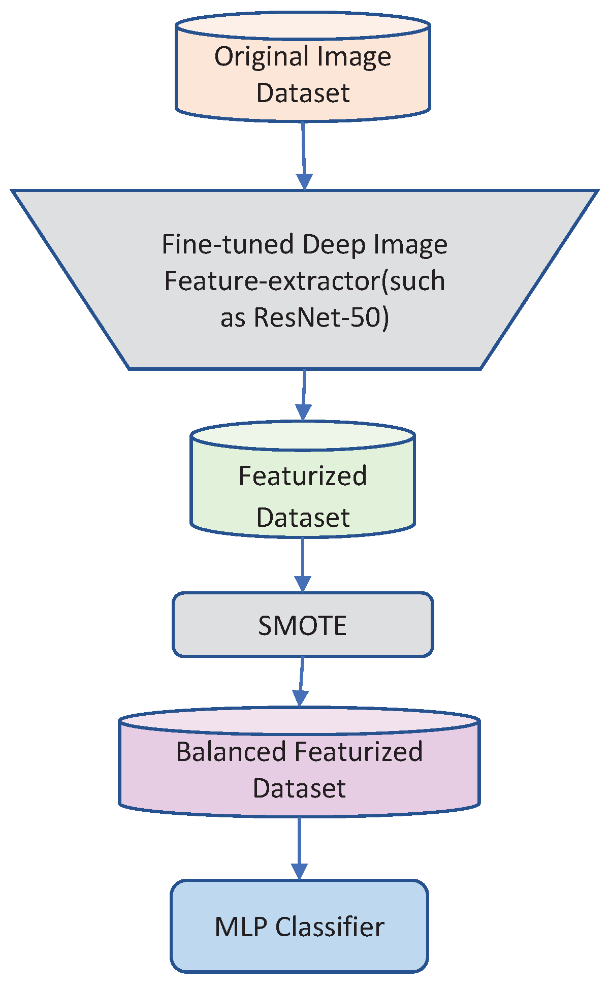
Except for noise, outliers, and sparse classes with substantial overlap, it is likely that new samples would not significantly deviate from the class distributions if the neighborhood is maintained modestly (i.e., as a size of 5). SMOTE, initially made to work with vector data sets without images, may also be used with images [34]. Several variants of SMOTE have been suggested accordingly [35,36]. We graphically demonstrate how SMOTE can be combined with a deep classifier in Figure 2.

2.2.2. Major-to-Minor Translation (M2m)

M2m is an oversampling technique for imbalance classification that uses adversarial noise perturbations to “transfer” images from majority classes to minor classes [26]. On the imbalance data set, M2m initially trains a classifier likely to become a specialist for the majority class. The majority class specialist classifier is then successfully deceived by randomly choosing an instance from the majority class and repeatedly subjecting it to noise perturbation. It is, therefore, possible to populate that class using this perturbed instance, which the classifier of the majority class has identified as an instance of a specific minority class. This process is repeated when a balanced data set is created. This strategy works very well for learning more generalizable features in unbalanced learning because it simultaneously takes advantage of the more detailed information in the majority samples while not relying too much on the minority data.

2.2.3. Generative Adversarial Networks

Choosing one GAN model from the numerous and expanding options is challenging. DCGAN consolidates GAN with CNN and due to DCGAN’s extensive use in numerous applications, including medical applications, and its propensity to accurately capture the fine details of real images, we chose to employ it. DCGAN produces a series of restrictions on CNN’s backbone network to enable it to be stably trained and use learned feature representations to classify images. A discriminative network and a generative network make up the two neural networks that make up DCGAN. DCGAN improves the qualities of generated images by carrying out the subsequent procedures. First, DCGAN uses stridden convolutions on the discriminator and fractional stride convolutions on the generator to replace the pooling layers. CNN is typically used to extract features. The discriminator network categorizes the original and newly formed images by the generator DCNN while the generator DCNN up-samples a vector of random noise to produce new images that are comparable to the training data. Second, the batch normalization (BN) approach is used by DCGAN to address the gradient disappearing issue. The BN approach limits the generator from collecting all samples to the equivalent point, resolves improper initializations, and carries the gradient to each layer. The network, which is employed in both the generator and the discriminator, is more stable when batch normalization is used. Lastly, DCGAN employs a variety of activation functions, such as leakyReLU and ReLU activation function. Tanh activation is used in the generator output, ReLU activation is used in the remaining layers of the generator, and Leaky ReLU activation is used in all of the discriminator’s layers. In applications involving medical image processing, DCGAN is among the most productive image augmentation methods [37].
The training model environment for DCGAN was a NVIDIA® RTX A6000 (48 GB) GPU with an Intel® Xeon® Gold 6246R Processor. Furthermore, our method is implemented in TensorFlow [38]. The generative network and discriminative network are trained with Adam [27] optimizer with β 1 = 0:5, β 2 = 0:999 and a learning rate of 0.0001. The batch size is 32 and the training set is set to 2000 epochs. The synthetic images generated by DCGAN were used for training and mixed with the real image to improve the classification accuracy.

2.3. Deep Classifier Selection

A key design choice for the framework developed in this paper is the choice of the deep learning classifier. Due to their high accuracy and robustness, deep learning (DL) models, such as convolutional neural networks (CNN), have been more popular since 2012 for image classification, image segmentation, and object recognition applications. A unique kind of multi-layer neural network called a CNN can extract a hierarchy of features—in this case, image-derived features—directly from the pixels of an image without any prior processing.
In this study, we examine the classification performance of four well-researched deep learning classifiers—Inception-V3, Xception, ResNet-101, and ResNet-50. These deep learning classifiers are used to fully exploit multi-scale feature maps. The trade-offs between accuracy and training time were our deciding factors for selecting the variants of ResNet [39]. Additionally, Xception and Inception-V3 were selected due to their successful performance on small data sets and their ability to reduce computation time while retaining classification accuracy [40,41].

2.4. Data Preparation Phase

This experiment was conducted in a greenhouse at Texas A&M AgriLife Research—Dallas Center, TX, USA. Heirloom tomato variety was used in the experiment. Tomato seeds were planted in the grow cubes placed in the growth chamber throughout the period for the tomato seeds to mature into seedlings. After a 14 days interval, the tomato seedlings were transferred to a potty mix in the greenhouse. The temperature in the greenhouse is kept at 25 °C, the air humidity ranges from 50–80%, and uniform lighting is used. These conditions are all managed by the intelligent control system in the growth chamber and the greenhouse. The tomato plants were grown and managed normally in a greenhouse during the experiment without pesticides.

2.5. Disease Inoculation Procedure

Bacterial wilt is one of the most common diseases affecting tomatoes and other solanaceous plants. The disease caused by the bacterium “Ralstonia solanacearum” is one of the most destructive plant pathogens. The following procedure below illustrates how we infected the tomato plants with bacterial wilt to acquire our data sets. The Ralstonia solanacearum strain was cultured on Potato Dextrose Agar (PDA) media for seven days at room temperature. For inoculation, one liter of PDA was used to culture the Ralstonia solanacearum by shaking at 200 rpm for 16 h till OD600 to 2.0. Then the strain culture was collected by centrifuge at 8000× g for 20 min, then re-suspended with ddH2O to an OD600 of 1.0. 1 mL of the inoculum was inoculated into the vascular system using a 30 G syringe needle.
For the bacterial wilt disease to take effect in the plants, the greenhouse was maintained at the following measurements light (16/8 h light/dark), humidity (over 80%), and soil moisture (over 80%) [42]. The effect of bacterial wilt on the plant took effect after two days showing different symptoms including (1) sudden wilting of the entire plant beginning at the shoot apex, which is frequently seen during the day, (2) wilted plant showing browning of the vascular tissue at the basal portion of the stem, (3) flow of a white, milky strand of bacterial ooze from a freshly cut section of infected stem base when placed in water. The tomato plants were infected with Ralstonia solanacearum at approximately seven weeks after the tomato seedlings were transferred to a potty mix.

2.6. Image Acquisition

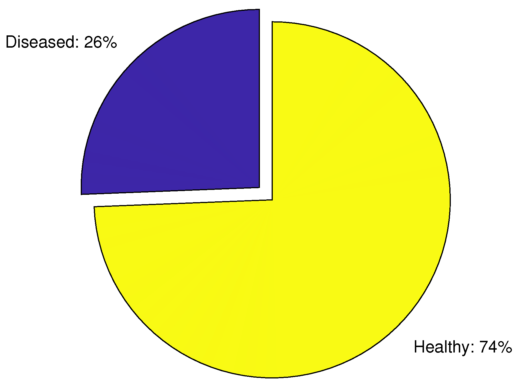
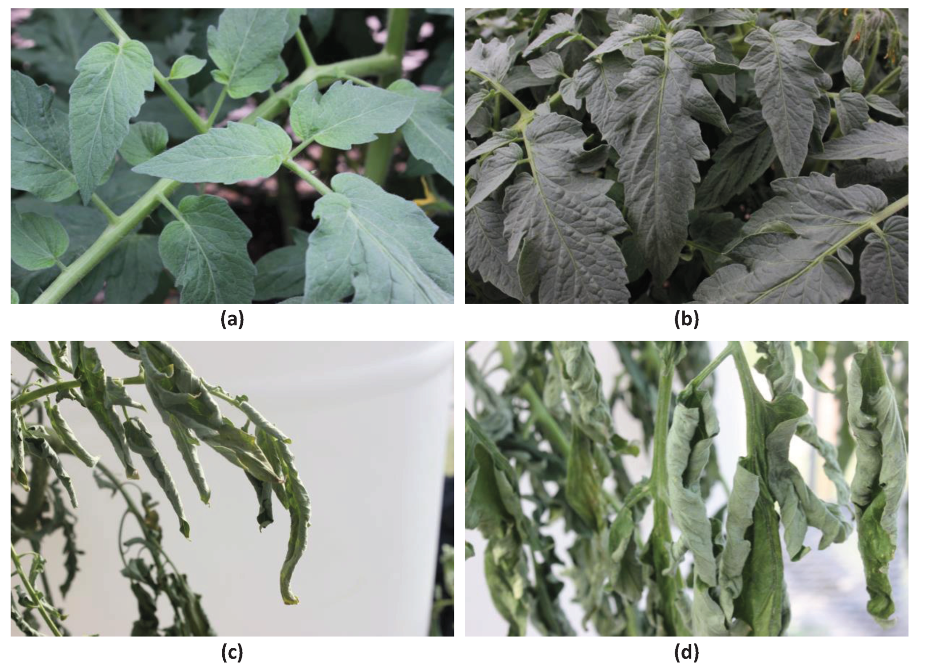
Images of the healthy and the infected plants were acquired with an RGB camera. We discovered a substantial imbalance between the diseased and healthy classes based on the images we collected. We classify healthy tomato leaves as the majority class and plant leaves that have contracted bacterial wilt as the minority class. The healthy plants have 9251 leaf labeled images, compared to 3186 for the diseased ones. The data distribution is shown in Figure 3. Figure 4 shows some examples of healthy and diseased plants.

3. Results and Discussion

3.1. Experimental Protocol

For performance evaluation, following criteria were used:

3.1.1. Average Classification Accuracy (ACA)

This is determined by averaging the recall values across all classes. When referring to recall, it is important to distinguish between predictions made by the classifier and actual predictions. According to Mullick et al. [43], ACA is not prejudiced against a particular class’s performance.

3.1.2. Precision

This quantifies the proportion of precise predictions compared to total predictions for each class. To elucidate, the precision for the i-th class is calculated by treating it as positive while treating others as negative. A plant disease detection system must have a high degree of precision to prevent false positive predictions from the classifier.

3.1.3. F1-Score

This combines precision and recall into one metric so that it is possible to see whether a high level of precision is simultaneously being accomplished with a good level of recall. The F1-score is essentially just the harmonic mean of recall and precision.

3.1.4. Area under Curve (AUC)

This measures the separability of a classification model for binary classification, and hence provides a summary of the entire range.
We select the parameter settings for the various preprocessing approaches based on the analysis in Section 3.2. We set the grid size at 10 for CLAHE, and the clip limit is 2. The sharpness factor for image sharpening is 4. The CL + SH is kept at the same value. The image preprocessing methods outlined above did not have any parameter adjusting for the remainder of the article.
SMOTE employs oversampling in the distributed feature space that the deep classifier has learnt (for example, the 2048-dimensional real-valued feature space that ResNet-50 uses to map an image). Therefore, in order to learn the mapping from the feature space to the class labels, we need an MLP identical to the one used in a deep classifier after the flattening procedure. Three fully connected hidden layers of 784, 256, and 128 neurons each make up the architecture of the MLP employed in SMOTE as the classifier. The classification layer utilizes a Soft-Max activation whereas the MLP uses Leaky-ReLU as the activation function with leakiness 0.1 at all the hidden layers. According to the established norm, the SMOTE algorithm’s neighborhood parameter size is 5. To locate the neighborhoods, we employ a direct euclidean distance. The settings we use for M2m are the same as those found in the article of Kim et al. [26].
In our study, we use a workstation running Windows 11 and equipped with the NVIDIA® RTX A6000 (48 GB) GPU on board. For low latency or high throughput, the GPU is made to speed up inference or predictions made by deep learning models. Hyperparameters are variables that define the structure of a convolutional network, and are typically the learning rate, epochs, batch size, number of layers, and activation functions, among others. In our work, the deep learning classifier runs for 200 epochs with a batch size of 64, a momentum of 0.9, and a learning rate of 0.001 during the fine-tuning process. For example, for ResNet-50, we made use of 49 convolutional layers and one fully connected layer with 16 residual blocks. In order to minimize any bias resulting from the randomness, the average and standard deviation values of the performance metrics are computed, and the procedures are repeated 10 times by using 10-fold cross validation; 60% of the data are used for training, 20% for validation, and 20% for testing.

3.2. Qualitative Analysis of Image Preprocessing Techniques

The potential comparative advantages or drawbacks of implementing the various preprocessing techniques can be revealed by visual examination of the output of those procedures. Such a study could help us narrow down many in-question preprocessing strategies that involve narrowing the parameter search space. For visual comparison purposes, we randomly choose diseased images from the data set, and evaluate the results after using the preprocessing technique in this section. We only make use of extra images to emphasize a certain property of potential abnormality for a preprocessing strategy.

3.2.1. AHE

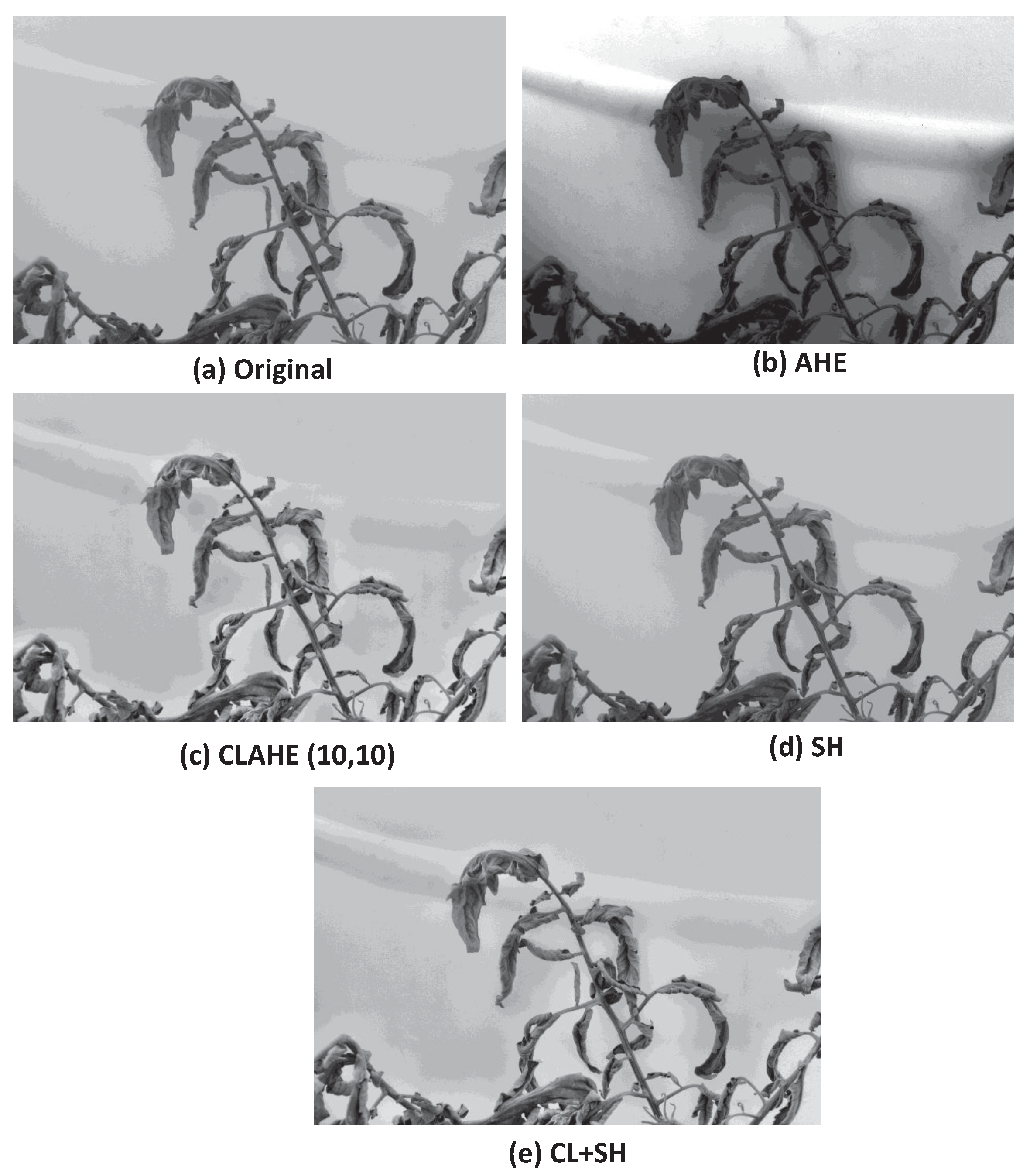
We can see from Figure 5b that AHE frequently tries to boost the image’s contrast by distorting it. A distortion such as this could cause the image to lose important details. The classifier may have serious problems as a result of the distortion. The AHE of the original image is displayed in Figure 5b.

3.2.2. CLAHE

Due to the fact that the other possibilities of clip limits 4 and 6 were observed to behave on the images similarly to AHE, we decided to adopt the clip limit of 2 for the CLAHE strategy. We investigate the impact of changing the grid size from 5, 10, 20, and 30 correspondingly. We see that CLAHE is often better than AHE, as shown in Figure 5. Additionally, the grid size is crucial for managing the trade-off between image enhancement and distortion. A larger grid size may lead to suppression, making it more challenging for the classifier to extract information. The procedure of highlighting some of the infected leaves in the dark region of the image, indicating anomalies, may not be possible with a smaller grid size. We discover that a ( 10 , 10 ) grid performs effectively. Figure 6 shows the CLAHE outputs with the clip limit set to 2 and the grid sizes of 5, 10, 20, and 30 correspondingly.

3.2.3. Image Sharpening

The effect of image sharpening can draw attention to the distinctive characteristics of diseased or infected leaves, but it can also increase noise inadvertently. The noise pixels in the images might become more intense and spread throughout their local area, generating sizable patches, among other serious difficulties. The distortion may mislead the classifier because it is likely to obscure the essential diagnostic traits. The sharpening of the original image is displayed in Figure 5d.

3.2.4. CLAHE + Sharpening (CL + SH)

Image sharpening can be an effective preprocessing method if its drawbacks can be met by coupling with other techniques, as described in Section 3.2.3. CLAHE is a viable option for enhancing the effectiveness of image sharpening. This is due to CLAHE’s ability to effectively intensify numerous artifacts in the infected leaves, regardless of their size, when its parameter settings are optimized. Given a CLAHE output, image sharpening can therefore ignore the noise that has been reduced and emphasize the amplified abnormal regions of the infected leaves even more.

3.2.5. Quality of the Augmented Data

The classifier’s performance is significantly influenced by the augmented image’s quality. When assessing the quality of the generated images, the following factors must be considered. The following requirements must be met: (1) overall image quality; (2) generated images must represent the target class; (3) no repetition in generated images. We discovered from the produced images that all requirements are met by SMOTE, M2m, and DCGAN.

3.3. Quantitative Analysis

In this section, we look into the potential performance improvements that could result from combining a deep learning classifier with various class imbalance techniques and preprocessing strategies.

3.3.1. Choosing the Base Classifier

We choose one classifier from a broad pool of thoroughly studied deep learning classifiers, including Inception-V3, Xception, ResNet-101, and ResNet-50, in the beginning stages of the quantitative experiment. With our data set, we looked at how well the classifiers performed in terms of ACA. A closer inspection of Table 1 reveals that on our data set, ResNet-50 achieves the best ACA while significantly outperforming its contenders making it a natural choice for our base classifier. This observation highlights the fact that depending on the application under concern, all classifiers may not be fair similarly to their performance on the natural image classification problems.

3.3.2. Impact of Class Handling Methods

Given that our data set is unbalanced, it may be advantageous to use a class-imbalance handling strategy beforehand so that the classifier would not be significantly burdened. We look into whether ResNet-50 with SMOTE, M2m, GAN-based algorithm can perform better than the unbalanced data set. In this experiment, two situations were assessed after resampling. In the first case, the healthy plants make up 50% of the data set, and in the second case, the healthy plants take up 60% of the data set. Table 2 and Table 3 shows the evaluation metrics for different approaches, which are based on a 10-fold cross-validation. We considered the classifier trained on the imbalance data set as the baseline. As a result, there is no replicated or generated data in the training data for the baseline. A closer look reveals that GAN-based approach outperforms SMOTE, M2m and the baseline in terms of all the precision, recall, F1-score, and AUC, which are particularly significant for the task at hand as shown in both Table 2 and Table 3. As accuracy ignores the smaller number of instances in each minority class, it is not the optimal metric for an imbalance data set. In situations such as this, precision and recall have frequently been employed to gauge a classifier’s effectiveness. Our GAN-based technique has a recall that is noticeably better than the baseline and marginally better than SMOTE and M2m. As this is our main goal, we can conclude that the GAN-based technique is effective at detecting the positive class. The GAN-based technique also maintains a good balance in detecting both classes because the F1-score and AUC are higher. The results clearly show that the GAN-based augmentation is superior to conventional sampling-based techniques at reducing the impact of the skewed data distribution. Table 2 and Table 3 also show that M2m, a recent feature-level augmentation method, which was created expressly to address class-imbalance issues in deep learning classifiers falls short of SMOTE in performance. This is because the adversarial learning of M2m is better suited for issues with extreme class imbalance, as described in [26]. The harder samples produced by M2m may make the classification task more challenging in low and moderate imbalance ratios cases where the class boundaries are slightly better defined. In addition, we see a small variation in the evaluation metrics of the sample techniques from the two scenarios. As the data set becomes more balanced, as seen in Table 2, the recall and AUC for all class imbalance approaches used slightly performs better. For the rest of the experiment, we continue with the first scenario (healthy plant occupying 50% of the data set).

3.3.3. Impact of Preprocessing Techniques

When the GAN-based approach is used with ResNet-50, we compare the performance of the different preprocessing strategies in Table 4 regarding ACA. As shown in Table 4, AHE falls short in enhancing the raw images because they tend to exacerbate noise. There is a slight improvement with regards to image sharpening because the noise enhances when the contours of the images have been highlighted to appear more prominent. Compared to the raw images, CLAHE produces some noticeable improvements. The CLAHE approach in CL + SH provides crucial preliminary improvements with noise suppression, then performance is significantly enhanced by image sharpening. Essentially, the study indicates the effectiveness of CL + SH in upgrading raw images for detecting plant diseases in addition to the quantitative performance correlating with the qualitative characteristics of the preprocessing methods.
We further investigate the data in terms of precision, recall, and F1-score as additional support for CL + SH. Table 4 shows that CL + SH preprocessing positively affects individual class-specific classification (diseased and healthy) and the overall performance of ResNet-50 classifiers for detecting plant diseases from raw images.
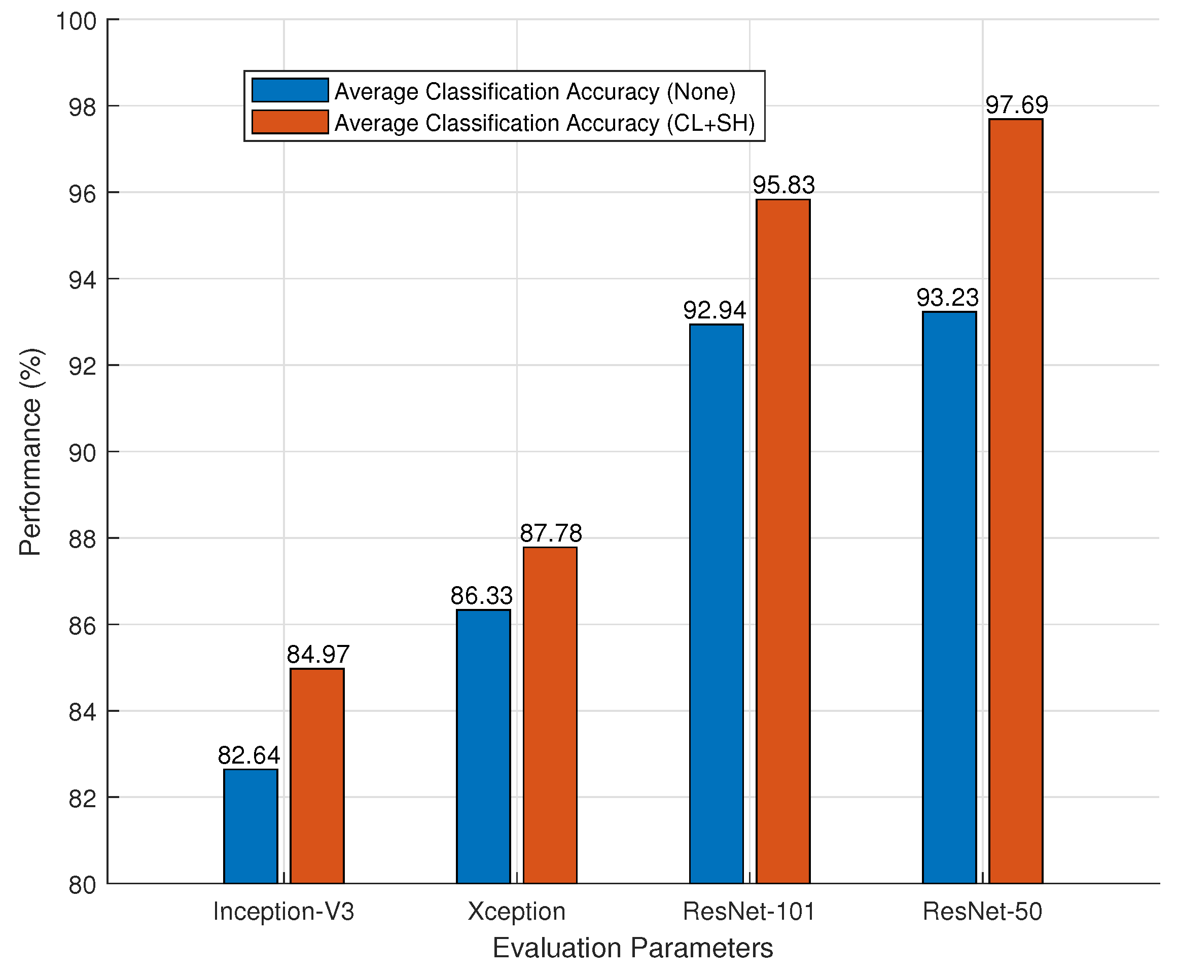
To determine whether CL + SH is truly generalizable in the sense that, when used in conjunction with a GAN-based strategy, it can improve the performance of other deep learning classifiers—Inception-V3, Xception, ResNet-101, and ResNet-50. Therefore, we conduct research on our data set in the following Table 5 by contrasting the performance of four weighted deep learning classifiers on unprocessed input (raw images) and preprocessed input (CL + SH). The table shows that CL + SH greatly outperforms raw images in terms of ACA, demonstrating its potential to enhance the functionality of deep learning classifiers. This is also evident from the Figure 7, which demonstrates that ResNet-50 outperforms other classifiers and that CL + SH outperforms raw images in terms of ACA.
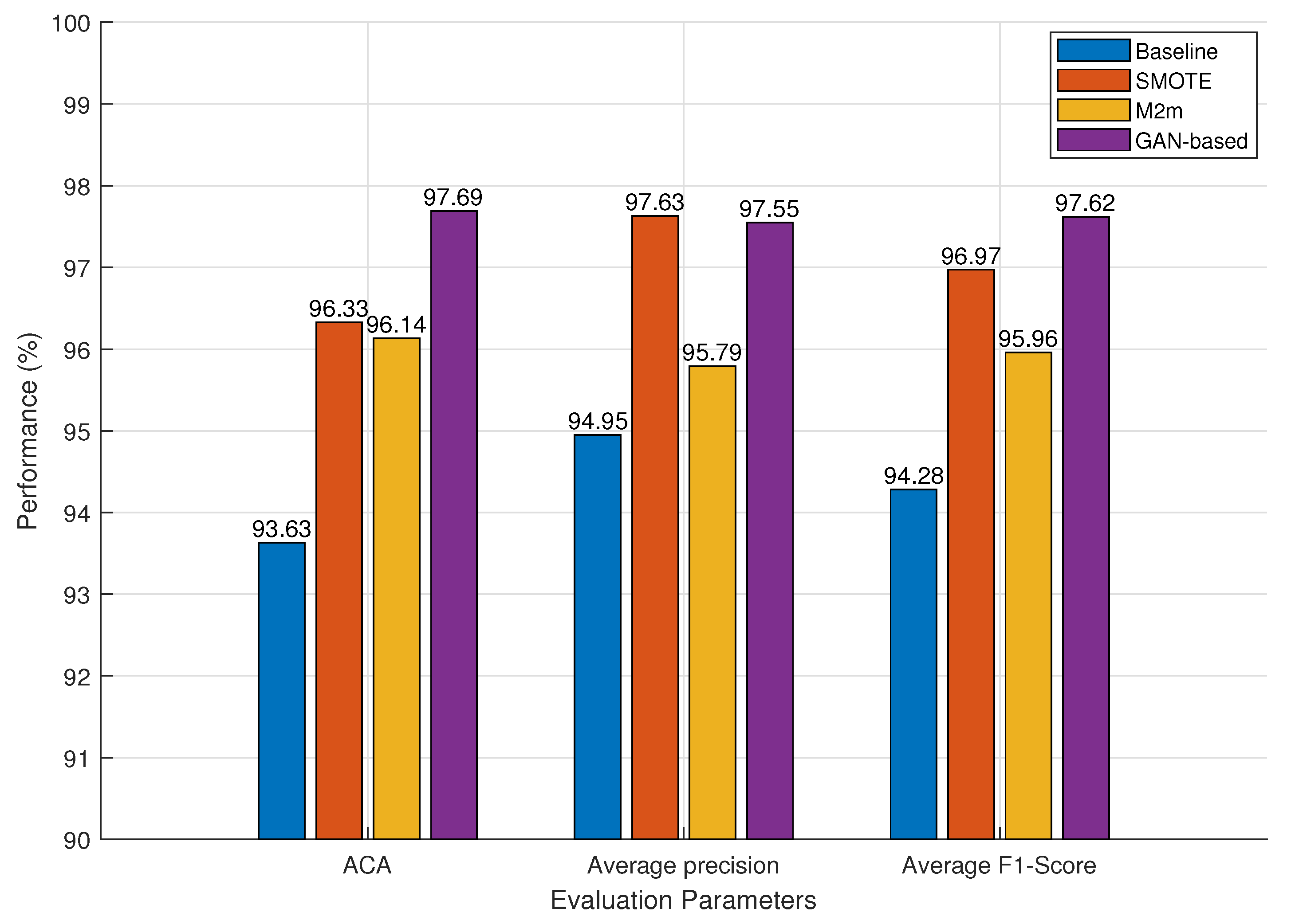
We further analyze our results when CL + SH is applied as the preprocessed input and ResNet-50 used as the deep learning classifier. Figure 8 displays the evaluation metrics ACA, average precision, and average F1-score values for various class imbalance approaches. Figure 8 demonstrates how the GAN-based method outperformed the data augmentation techniques used in this study. The SMOTE approach appears to be the top contender among the four in terms of average precision. As a result, SMOTE has a lower rate of misclassification for negative samples. The GAN-based strategy outperformed other approaches in terms of average F1-score and ACA, which are particularly crucial for the task at hand. The GAN-based strategy is superior to baseline and M2m, and marginally better than SMOTE, according to the ACA and average F1-score. Thus, we can conclude that GAN-based detection of both classes maintains a good equilibrium. In summary, we can draw the conclusion that it may always be advantageous for the classifier to resolve class imbalance when it arises.

3.3.4. Lessons Learned and Future Directions

This study empirically investigates the applicability of various preprocessing methods to perform noise reduction and diseases attributed anomaly enhancement in plant images. Furthermore, the use of general purpose deep classifiers leveraging transfer learning to address the scarcity of samples and employing class imbalance handling to counter the effect of distinct prevalence of diseases emphasizes the practical implementability of this study. In support of wider applicability, this study presents a general workflow of a disease diagnosis system where each component can be separately focused on according to need. In essence, the research work can be beneficial to several research communities working in computational intelligence, agricultural image analysis, and interdisciplinary topics.
Future expansion of the existing research effort may take many different forms. First, we stress the significance of reducing noise, which is prevalent, particularly during collection of images. However, a balance must be struck such that the irregularities in the infected images are not masked as a result of noise removal. Second, data sets on plant diseases with various symptoms will be utilized to further explain the influence of preprocessing and class imbalance techniques on deep learning classifiers. Third, further preprocessing and resampling procedures would be applied to create a more accurate comparative analysis.
Our preprocessing methods in this paper only applied non-learning based strategies. As a result, in our future work, we will carefully examine the effects of learning-based preprocessing techniques such as UNET and compare the outcomes with non-learning based techniques. Classification or segmentation performed on an imbalance and limited dataset may have a considerable negative impact on deep learning classifiers. As a result, in addition to the original data, synthetic images that are consistent with the original data are needed to solve this problem. This implies that synthetic image generation holds a promising future and has a scope of opening multiple possibilities in the agricultural imaging domain. In addition, we will investigate further generative adversarial networks in the future, such as least squares generative adversarial networks (LSGAN) and Wasserstein generative adversarial networks (WGAN). We shall comprehend the feature of the synthetic image that influences the technique through a model trained on synthetic images of various sizes. We will design a new optimized GAN to generate diseased images and compare it with the existing GANs in our future works. Future studies will experiment with more synthetic image generation techniques combined with Explainable AI (XAI).
Lastly, we propose to use energy-efficient edge computing devices in our future work to achieve real-time plant disease diagnosis using edge-AI while maintaining mean average precision and satisfying real-time requirements. The proper technologies to leverage for an AI-based application are edge computing and IoT, and doing so significantly reduces costs even though implementation is still far from simple and straightforward.

4. Conclusions

In this study, we explicitly examine the case of bacterial wilt disease detection using preprocessing techniques and class imbalance methods. AHE, CLAHE, image sharpening, hybrid approach, and a balanced data set of plant disease produced from various resampling approaches such as SMOTE, M2m, and GAN-based have all been used in an experimental evaluation of the performance of deep learning classifiers. Our findings show that the GAN-based strategy performs better than SMOTE and M2m. A GAN-based technique introduces variance into the samples, which makes it simpler for the classifier to identify classification boundaries. Additionally, the capacity of the GAN-based generative strategy to avoid overfitting shows its superiority to sampling-based approaches in the goal of detecting plant diseases. Various deep learning classifiers were used to analyze the results. To further explore, we demonstrate how applying image sharpening to the input images after CLAHE, can enhance a deep learning classifier’s performance. According to our experimental research, ResNet-50 outperforms ResNet-101 on a basic data set with relatively distinct classes, consistent with the work of Magalhães et al. [44]. In addition, ResNet-50 outperformed other investigated deep learning classifiers. We also observe that ResNet-50 performs faster during training, and is a better fit compared to ResNet-101 and other deep learning classifiers.

Author Contributions

Conceptualization, M.O.O. and A.Z.; methodology, M.O.O.; formal analysis, M.O.O.; investigation, M.O.O.; writing—original draft preparation, M.O.O.; writing—review and editing, A.Z.; visualization, M.O.O.; funding acquisition, A.Z. All authors have read and agreed to the published version of the manuscript.

Funding

This research was funded by Texas Department of Agriculture (Specialty Crop Block Grant Agreement # GSC2022105). This research was partially supported in part by the United States Department of Agriculture (USDA)’s National Institute of Food and Agriculture (NIFA) Federal Appropriations under TEX09954 and Accession No. 7002248. This publication was also supported by Texas A&M AgriLife Research, Vegetable and Fruit Improvement Center (VFIC), and the Hatch program of the USDA-NIFA.

Data Availability Statement

Not applicable.

Conflicts of Interest

The authors declare no conflict of interest.

References

  1. Bai, Y.; Xiong, Y.; Huang, J.; Zhou, J.; Zhang, B. Accurate prediction of soluble solid content of apples from multiple geographical regions by combining deep learning with spectral fingerprint features. Postharvest Biol. Technol. 2019, 156, 110943. [Google Scholar] [CrossRef]
  2. World Health Organization. The State of Food Security and Nutrition in the World 2018: Building Climate Resilience for Food Security and Nutrition; Food & Agriculture Org: Rome, Italy, 2018.
  3. Ojo, M.O.; Zahid, A. Deep learning in controlled environment agriculture: A review of recent advancements, challenges and prospects. Sensors 2022, 22, 7965. [Google Scholar] [CrossRef] [PubMed]
  4. Singh, A.K.; Ganapathysubramanian, B.; Sarkar, S.; Singh, A. Deep learning for plant stress phenotyping: Trends and future perspectives. Trends Plant Sci. 2018, 23, 883–898. [Google Scholar] [CrossRef] [PubMed] [Green Version]
  5. Mohanty, S.P.; Hughes, D.P.; Salathé, M. Using deep learning for image-based plant disease detection. Front. Plant Sci. 2016, 7, 1419. [Google Scholar] [CrossRef] [PubMed] [Green Version]
  6. Ferentinos, K.P. Deep learning models for plant disease detection and diagnosis. Comput. Electron. Agric. 2018, 145, 311–318. [Google Scholar] [CrossRef]
  7. Caldwell, D.; Kim, B.-S.; Iyer-Pascuzzi, A.S. Ralstonia solanacearum differentially colonizes roots of resistant and susceptible tomato plants. Phytopathology 2017, 107, 528–536. [Google Scholar] [CrossRef] [PubMed] [Green Version]
  8. Unay, D.; Gosselin, B.; Kleynen, O.; Leemans, V.; Destain, M.-F.; Debeir, O. Automatic grading of bi-colored apples by multispectral machine vision. Comput. Electron. Agric. 2011, 75, 204–212. [Google Scholar] [CrossRef] [Green Version]
  9. Gavhale, K.R.; Gawande, U.; Hajari, K.O. Unhealthy region of citrus leaf detection using image processing techniques. In Proceedings of the International Conference for Convergence for Technology-2014, Pune, India, 6–8 April 2014; pp. 1–6. [Google Scholar]
  10. Vetal, S.; Khule, R. Tomato plant disease detection using image processing. Int. J. Adv. Res. Comput. Commun. Eng. 2017, 6, 293–297. [Google Scholar] [CrossRef]
  11. Sun, Y.; Kamel, M.S.; Wong, A.K.; Wang, Y. Cost-sensitive boosting for classification of imbalanced data. Pattern Recognit. 2007, 40, 3358–3378. [Google Scholar] [CrossRef]
  12. Japkowicz, N. Supervised versus unsupervised binary-learning by feedforward neural networks. Mach. Learn. 2001, 42, 97–122. [Google Scholar] [CrossRef] [Green Version]
  13. Ling, C.X.; Sheng, V.S. Cost-sensitive learning and the class imbalance problem. Encycl. Mach. Learn. 2008, 2011, 231–235. [Google Scholar]
  14. Johnson, J.M.; Khoshgoftaar, T.M. Survey on deep learning with class imbalance. J. Big Data 2019, 6, 27. [Google Scholar] [CrossRef] [Green Version]
  15. Ling, C.X.; Li, C. Data mining for direct marketing: Problems and solutions. KDD 1998, 98, 73–79. [Google Scholar]
  16. Chawla, N.V.; Bowyer, K.W.; Hall, L.O.; Kegelmeyer, W.P. SMOTE: Synthetic minority over-sampling technique. J. Artif. Res. 2002, 16, 321–357. [Google Scholar] [CrossRef]
  17. Janowczyk, A.; Madabhushi, A. Deep learning for digital pathology image analysis: A comprehensive tutorial with selected use cases. J. Pathol. Inform. 2016, 7, 29. [Google Scholar] [CrossRef]
  18. Zhang, C.; Zhou, P.; Li, C.; Liu, L. A convolutional neural network for leaves recognition using data augmentation. In Proceedings of the 2015 IEEE International Conference on Computer and Information Technology; Ubiquitous Computing and Communications; Dependable, Autonomic and Secure Computing; Pervasive Intelligence and Computing, Liverpool, UK, 26–28 October 2015; pp. 2143–2150. [Google Scholar]
  19. Pan, Z.; Yu, W.; Yi, X.; Khan, A.; Yuan, F.; Zheng, Y. Recent progress on generative adversarial networks (gans): A survey. IEEE Access 2019, 7, 36322–36333. [Google Scholar] [CrossRef]
  20. Mai, G.; Cao, K.; Yuen, P.C.; Jain, A.K. On the reconstruction of face images from deep face templates. IEEE Trans. Pattern Anal. Mach. Intell. 2018, 41, 1188–1202. [Google Scholar] [CrossRef] [Green Version]
  21. Hu, G.; Wu, H.; Zhang, Y.; Wan, M. A low shot learning method for tea leaf’s disease identification. Comput. Electron. Agric. 2019, 163, 104852. [Google Scholar] [CrossRef]
  22. Saikawa, T.; Cap, Q.H.; Kagiwada, S.; Uga, H.; Iyatomi, H. Aop: An anti-overfitting pretreatment for practical image-based plant diagnosis. In Proceedings of the 2019 IEEE International Conference on Big Data (Big Data), Los Angeles, CA, USA, 9–12 December 2019; pp. 5177–5182. [Google Scholar]
  23. Mirza, M.; Osindero, S. Conditional generative adversarial nets. arXiv 2014, arXiv:1411.1784. [Google Scholar]
  24. Tian, Y.; Yang, G.; Wang, Z.; Li, E.; Liang, Z. Detection of apple lesions in orchards based on deep learning methods of cyclegan and yolov3-dense. J. Sens. 2019, 2019, 7630926. [Google Scholar] [CrossRef]
  25. Cap, Q.H.; Uga, H.; Kagiwada, S.; Iyatomi, H. Leafgan: An effective data augmentation method for practical plant disease diagnosis. IEEE Trans. Autom. Sci. Eng. 2020, 1258–1267. [Google Scholar] [CrossRef]
  26. Kim, J.; Jeong, J.; Shin, J. M2m: Imbalanced classification via major-to-minor translation. In Proceedings of the IEEE/CVF Conference on Computer Vision and Pattern Recognition, Seattle, WA, USA, 13–19 June 2020; pp. 13896–13905. [Google Scholar]
  27. Radford, A.; Metz, L.; Chintala, S. Unsupervised representation learning with deep convolutional generative adversarial networks. arXiv 2015, arXiv:1511.06434. [Google Scholar]
  28. Pizer, S.M.; Amburn, E.P.; Austin, J.D.; Cromartie, R.; Geselowitz, A.; Greer, T.; ter Haar Romeny, B.; Zimmerman, J.B.; Zuiderveld, K. Adaptive histogram equalization and its variations. Comput. Vis. Graph. Image Process. 1987, 39, 355–368. [Google Scholar] [CrossRef]
  29. Reza, A.M. Realization of the contrast limited adaptive histogram equalization (clahe) for real-time image enhancement. J. VLSI Signal Process. Syst. Signal Image Video Technol. 2004, 38, 35–44. [Google Scholar] [CrossRef]
  30. Kubat, M.; Matwin, S. Addressing the curse of imbalanced training sets: One-sided selection. ICML 1997, 97, 179. [Google Scholar]
  31. Oksuz, K.; Cam, B.C.; Kalkan, S.; Akbas, E. Imbalance problems in object detection: A review. IEEE Trans. Pattern Anal. Mach. Intell. 2020, 43, 3388–3415. [Google Scholar] [CrossRef] [PubMed] [Green Version]
  32. Buda, M.; Maki, A.; Mazurowski, M.A. A systematic study of the class imbalance problem in convolutional neural networks. Neural Netw. 2018, 106, 249–259. [Google Scholar] [CrossRef] [Green Version]
  33. Drummond, C.; Holte, R.C. C4. 5, class imbalance, and cost sensitivity: Why under-sampling beats over-sampling. Workshop Learn. Imbalanced Datasets II 2003, 11, 1–8. [Google Scholar]
  34. Nafi, N.M.; Hsu, W.H. Addressing class imbalance in image-based plant disease detection: Deep generative vs. sampling-based approaches. In Proceedings of the 2020 International Conference on Systems, Signals and Image Processing (IWSSIP), Niteroi, Brazil, 1–3 July 2020; pp. 243–248. [Google Scholar]
  35. Han, H.; Wang, W.-Y.; Mao, B.-H. Borderline-smote: A new over-sampling method in imbalanced data sets learning. In Proceedings of the International Conference on Intelligent Computing, Hefei, China, 23–26 August 2005; pp. 878–887. [Google Scholar]
  36. He, H.; Bai, Y.; Garcia, E.; Li, S.A. Adaptive synthetic sampling approach for imbalanced learning. In Proceedings of the 2008 IEEE International Joint Conference on Neural Networks (IEEE World Congress on Computational Intelligence), Hong Kong, China, 1–8 June 2008. [Google Scholar]
  37. Bang, S.; Baek, F.; Park, S.; Kim, W.; Kim, H. Image augmentation to improve construction resource detection using generative adversarial networks, cut-and-paste, and image transformation techniques. Autom. Constr. 2020, 115, 103198. [Google Scholar] [CrossRef]
  38. Abadi, M.; Barham, P.; Chen, J.; Chen, Z.; Davis, A.; Dean, J.; Devin, M.; Ghemawat, S.; Irving, G.; Isard, M.; et al. Tensorflow: A system for large-scale machine learning. OSDI 2016, 16, 265–283. [Google Scholar]
  39. He, K.; Zhang, X.; Ren, S.; Sun, J. Deep residual learning for image recognition. In Proceedings of the IEEE Conference on Computer Vision and Pattern Recognition, Las Vegas, NV, USA, 27–30 June 2016; pp. 770–778. [Google Scholar]
  40. Chao, X.; Hu, X.; Feng, J.; Zhang, Z.; Wang, M.; He, D. Construction of apple leaf diseases identification networks based on xception fused by se module. Appl. Sci. 2021, 11, 4614. [Google Scholar] [CrossRef]
  41. Wang, C.; Chen, D.; Hao, L.; Liu, X.; Zeng, Y.; Chen, J.; Zhang, G. Pulmonary image classification based on inception-v3 transfer learning model. IEEE Access 2019, 7, 146533–146541. [Google Scholar] [CrossRef]
  42. Singh, D.; Yadav, D.; Sinha, S.; Choudhary, G. Effect of temperature, cultivars, injury of root and inoculums load of ralstonia solanacearum to cause bacterial wilt of tomato. Arch. Phytopathol. Plant Prot. 2014, 47, 1574–1583. [Google Scholar] [CrossRef]
  43. Mullick, S.S.; Datta, S.; Dhekane, S.G.; Das, S. Appropriateness of performance indices for imbalanced data classification: An analysis. Pattern Recognit. 2020, 102, 107197. [Google Scholar] [CrossRef]
  44. Magalhães, S.A.; Castro, L.; Moreira, G.; Santos, F.N.D.; Cunha, M.; Dias, J.; Moreira, A.P. Evaluating the single-shot multibox detector and yolo deep learning models for the detection of tomatoes in a greenhouse. Sensors 2021, 21, 3569. [Google Scholar] [CrossRef]
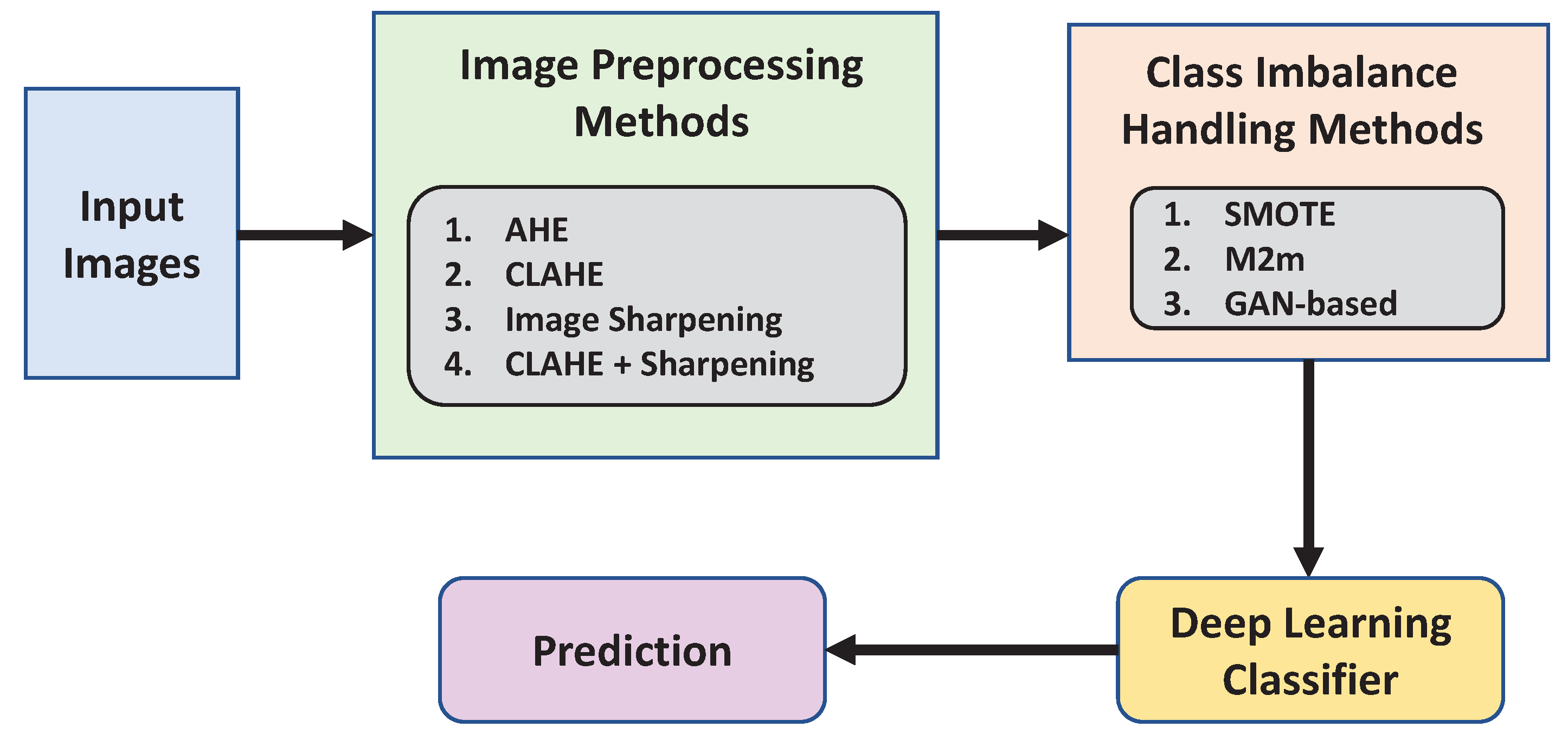
Figure 1. The workflow of a plant disease detection system. First, image preprocessing techniques improve the images, and then class imbalance techniques address the inequalities of the minority class. A deep learning classifier provides the prediction. Here, we also list the various techniques we consider for this study for each component.
Agronomy 13 00887 g001
Figure 2. The figure demonstrates the integration of SMOTE into a deep learning classifier. First, the images are used to fine-tune a deep image classifier (for example, ResNet-50). The classifier’s classification layers are then removed, enabling it to function as a feature extractor. The customized deep feature extractor then maps the images to the distributed feature space. This featurized data set is subjected to SMOTE in order to increase synthetic minority class instances in order to minimize the impact of class imbalance. The multi-layer perceptron (MLP) is then used to map the class labels to the final featurized data set balanced by SMOTE.
Agronomy 13 00887 g002
Figure 3. Distribution of the images before resampling.
Agronomy 13 00887 g003
Figure 4. Examples of the healthy plants in (a,b) and the diseased plants in (c,d).
Agronomy 13 00887 g004
Figure 5. The output of the image preprocessing methods applied to a random image.
Agronomy 13 00887 g005
Figure 6. CLAHE outputs with the clip limit set to 2 and the grid sizes of 5, 10, 20, and 30 correspondingly.
Agronomy 13 00887 g006
Figure 7. Performance evaluation in terms of ACA by deep learning classifiers coupled with GAN-based when CL + SH is used for preprocessing.
Agronomy 13 00887 g007
Figure 8. Metrics for evaluating different class imbalance approaches when CL + SH is applied as the preprocessed input and ResNet-50 used as the deep learning classifier (Average for 10-fold cross validation).
Agronomy 13 00887 g008
Table 1. Performance comparison of the four state-of-the-art deep learning classifiers in terms of ACA (average for 10-fold cross validation).
ClassifierACA (%)
Inception-V381.73 ± 0.672
Xception85.49 ± 0.231
ResNet-10192.02 ± 0.055
ResNet-5092.15 ± 0.04
Table 2. Performance metrics of the class imbalance techniques with 50% healthy plants and 50% diseased plants (Average for 10-fold cross validation).
MethodPrecisionRecallF1-ScoreAUCAccuracy
Baseline84.39 ± 0.20592.15 ± 0.0488.23 ± 0.13889.33 ± 0.09590.03 ± 0.036
SMOTE90.13 ± 0.01792.87 ± 0.02191.47 ± 0.01694.69 ± 0.01593.12 ± 0.022
M2m89.72 ± 0.03692.59 ± 0.02991.12 ± 0.03493.16 ± 0.03792.55 ± 0.035
GAN-based93.70 ± 0.01793.23 ± 0.01693.46 ± 0.01496.12 ± 0.01195.99 ± 0.013
Table 3. Performance metrics of the class imbalance techniques with 60% healthy plants and 40% diseased plants (Average for 10-fold cross validation).
MethodPrecisionRecallF1-ScoreAUCAccuracy
Baseline84.39 ± 0.20592.15 ± 0.0488.23 ± 0.13889.33 ± 0.09590.03 ± 0.036
SMOTE91.53 ± 0.02692.73 ± 0.03192.12 ± 0.02792.22 ± 0.02890.87 ± 0.028
M2m88.15 ± 0.05892.49 ± 0.04190.24 ± 0.03990.51 ± 0.03186.91 ± 0.064
GAN-based91.99 ± 0.01992.97 ± 0.0292.47 ± 0.01993.28 ± 0.02495.62 ± 0.021
Table 4. ResNet-50 classification with GAN-based on different preprocessing techniques.
Preprocessing TechniquesClassesOverall
IndicesHealthyDiseaseIndicesPerformance (%)
AHEPrecision (%)87.23 ± 0.09283.97 ± 0.256Average Precision85.60 ± 0.101
Recall (%)86.13 ± 0.11684.09 ± 0.354ACA85.11 ± 0.158
F1-Score (%)86.67 ± 0.18384.02 ± 0.392Average F1-score85.35 ± 0.279
CLAHEPrecision (%)96.85 ± 0.0195.82 ± 0.011Average Precision96.33 ± 0.01
Recall (%)95.59 ± 0.01296.27 ± 0.009ACA95.93 ± 0.01
F1-score (%)96.21 ± 0.00996.04 ± 0.009Average F1-score96.13 ± 0.009
SHPrecision (%)94.72 ± 0.01993.86 ± 0.017Average Precision94.29 ± 0.025
Recall (%)93.95 ± 0.02193.32 ± 0.025ACA93.63 ± 0.022
F1-score (%)94.33 ± 0.02393.59 ± 0.02Average F1-score93.96 ± 0.016
CL + SHPrecision (%)97.71 ± 0.00997.39 ± 0.01Average Precision97.55 ± 0.009
Recall (%)98.27 ± 0.00797.11 ± 0.007ACA97.69 ± 0.008
F1-score (%)97.99 ± 0.00797.24 ± 0.008Average F1-score97.62 ± 0.008
NonePrecision (%)94.54 ± 0.01192.86 ± 0.013Average Precision93.70 ± 0.017
Recall (%)93.82 ± 0.01192.64 ± 0.013ACA93.23 ± 0.016
F1-score (%)94.18 ± 0.01292.75 ± 0.012Average F1-score93.46 ± 0.014
Table 5. Performance evaluation in terms of ACA by deep learning classifiers in combination with GAN-based technique when CL + SH is used for preprocessing.
ClassifierACA (CL + SH) (%)ACA (None) (%)
Inception-V384.97 ± 0.34282.64 ± 0.552
Xception87.78 ± 0.13286.33 ± 0.159
ResNet-10195.83 ± 0.01992.94 ± 0.031
ResNet-5097.69 ± 0.00893.23 ± 0.016
Disclaimer/Publisher’s Note: The statements, opinions and data contained in all publications are solely those of the individual author(s) and contributor(s) and not of MDPI and/or the editor(s). MDPI and/or the editor(s) disclaim responsibility for any injury to people or property resulting from any ideas, methods, instructions or products referred to in the content.