Article

Exploring the Macroscopic Properties of Humic Substances Using Modeling and Molecular Simulations

Institute of Molecular Modeling and Simulation, Department of Material Sciences and Process Engineering, University of Natural Resources and Life Sciences, Vienna (BOKU), Muthgasse 18, 1190 Vienna, Austria
*
Author to whom correspondence should be addressed.
Agronomy 2023, 13(4), 1044; https://doi.org/10.3390/agronomy13041044
Submission received: 15 February 2023 / Revised: 24 March 2023 / Accepted: 27 March 2023 / Published: 1 April 2023

Abstract

:
Soil organic matter (SOM) is composed of a complex and heterogeneous mixture of organic compounds, which poses a challenge in understanding it on an atomistic level. Based on the progress of molecular dynamics simulations and our efforts to create molecular systems that resemble SOM, in this work, we expanded our knowledge of SOM through the use of humic substances (HSs). Specifically, we studied the standardized samples of HS of the International Humic Substances Society (IHSS). This society provided the elemental and organic composition used as input parameters for our Vienna Soil Organic Matter Modeler 2 (VSOMM2). We modeled and simulated different HS samples from various sources, including soil, peat, leonardite, and blackwater river. In order to compare between different HS, we reduced the organic composition information to two principal components, which are associated principally with the amount of carboxyl and aromatic groups in the HS, denominated as PC acid and PC arom , respectively. We performed a plethora of analyses to characterize the structure and dynamics of the systems, including the total potential energy, density, diffusion, preferential solvation, hydrogen bonds, and salt bridges. In general terms, at the water content value of 0.2, we observed that most properties depend on the carboxyl group protonation state. The Coulombic interactions from this ionic specie and the interaction with cations determine the overall behavior of the studied systems. Furthermore, the type of cations and the pH influence those properties. This study exemplifies the importance of molecular dynamics to explain macroscopic properties from the structure and dynamics of the molecules modeled, such as the interaction network, i.e., hydrogen bonds or salt bridges of molecules presented in the system and their mobility.

1. Introduction

Soil organic matter (SOM) is composed of a complex and heterogeneous mixture of organic compounds as a result of different factors, such as plant and microbial inputs, parent materials, climate, and external disturbances [1,2,3]. The study of soil organic matter is challenging in terms of the multiple variables to consider, which requires an interdisciplinary research approach. Multiple questions arise related to the structure, water accessibility, interfaces, and reactivity of different kinds of soil organic matter [1,4]. In terms of the atomistic interactions, it is imperative to understand the interplay of interactions between organic compounds, ion species, and water, and how these interactions can be extrapolated to macroscopic properties. Our understanding of the properties and behavior of SOM is crucial in addressing important questions related to the impacts of pollutants and pesticides in the carbon cycle and their effects on global warming [5,6,7,8].
Humic substances (HSs) have been proposed to be the principal component of SOM and correspond to organic compounds formed by the humification process of plant and microbial remains [9]. The precise properties and structure of HSs are determined based on the water content, soil source, and extraction methods [10,11]. New experiments have demonstrated the complexity of SOM and the interconnectivity with the mineral matrix, making a significant leap between the being and essence of the humic substance definition. Despite this discussion, the extracted samples and their standardization have facilitated a systematic understanding of SOM for decades [10].
An alkaline solution is used to extract HSs from the soil. The alkaline solution usually corresponds to a sodium hydroxide (NaOH) solution that solubilizes soil organic compounds via the ionization of carboxylic and phenolic groups. The subsequent re-acidification of the solution produces a precipitate called humic acid (HA) and a supernatant called fulvic acid (FA).
The standardization of humic substances has been facilitated thanks to the International Humic Substances Society (IHSS. Available online: https://humic-substances.org/, accessed on 13 December 2021). The collection of these samples is accompanied by information about their elemental composition, 13 C NMR Carbon distribution, and acidic functional groups, among others [12]. This permits us to gain insight into the chemical structure of SOM in general terms.
This information can be used to model and simulate the molecular structure of SOM. The use and power of molecular models have increased tremendously in combination with molecular simulations that can predict the dynamics and thermodynamic properties of constituting molecules. This simulation technique captures the motion of atoms, and the trajectory thus generated represents statistical mechanics ensembles, which can be used to extract macroscopic observables. Each molecular dynamics simulation can be considered a performed experiment in silico [13]. This tool allows us to understand how macroscopic properties are linked with the chemical structures and compositions of SOM.
Advances related to molecular dynamics have demonstrated the importance of the aggregation of soil organic matter. TNB models and VSOMM models have been used for molecular simulation to describe the aggregation of humic substances and the interaction between carboxyl groups and positive ions [14,15,16].
VSOMM models have been used to obtain thermodynamic properties, such as density, diffusion coefficients, and dielectric constant [16,17,18,19]. For example, the effects of compactness and water content and their relevance in hydrogen bonding and the absorption of small molecules were studied. Previous models of VSOMM focused on one of the standard humic substance samples from the IHSS society, called leonardite humic acid (LHA). The use of LHA was chosen because of its well-documented composition [20] as well as its sorption capacity with different organic compounds [21], making it a good candidate for studies with molecular dynamics and free-energy calculations. Therefore, it is relevant to explore how other humic substances behave as a function of their organic composition.
In this work, which was part of the doctoral thesis of Yerko Escalona [22], we used the Vienna Soil Organic Matter Modeler 2 (VSOMM2) [23] to create models of 15 different samples of the standard humic substances. The humic substances, humic acids or fulvic acids, correspond to different stocks (determined with roman numbers) of four source samples taken from soil, peat, leonardite, and blackwater river, denominated as Elliott Soil, Pahokee Peat, Leonardite, and Suwannee River, respectively. We extensively simulate the generated systems under different conditions and analyze their structure, dynamics, and thermodynamics of humic substances. This work expands our understanding of soil organic matter at a molecular level in terms of its chemical composition and macroscopic properties.

2. Materials and Methods

We used the Vienna Soil Organic Matter Modeler (VSOMM2) [23] to create four independent models for each of the standard humic substances of the International Humic Substances Society (IHSS), following their elemental and organic composition. For each model, we generated systems containing water and counterions. The water content of the system, in terms of the fraction of heavy atoms in the system, is 0.2. Conditions include systems at neutral and acidic pH, as well as the usage of sodium (Na + ) and calcium (Ca 2 + ) as a counterion. Systems were simulated by using molecular dynamics (MD) with the GROMOS software package and the united atom GROMOS force field 54A7 [24,25], which is a force field designed to reproduce thermodynamic properties, such as the density or heat of vaporization of organic compounds in the condensed phase [26,27], arguably allowing for realistic modeling of the organic matter of soil [23]. We tested different equilibration schemes for our system [19], which permit us to obtain equilibrated trajectories for further analysis. The structure and dynamics of the simulated systems were analyzed using the gromos++ set of analysis programs [28]. Analyses comprehend macroscopic properties, such as density, total potential energy, dielectric constant, absorption of methane, and diffusion coefficient. Furthermore, we analyze the individual molecular species (humic substances, cations, and water) and their preferential solvation, number of hydrogen bonds, and number of salt bridges. For a clear comprehension of the different system properties of different humic substances, it was necessary to apply a principal component analysis (PCA) in order to plot the data with the two main principal components, denominated as aromaticity (PC arom ) and acidity (PC acid ) of the humic substances. For more details, see Appendix A.

3. Results

3.1. Principal Component Analysis of the Organic Composition

To correlate the observable macroscopic properties of our models with their chemical composition, we tried a different approximation, for instance, grouping data by their source type or between humic or fulvic acid. However, due to the broad spectrum of organic composition, even from the same source and extraction fraction, it is difficult to classify the samples meaningfully. For this reason, we decided to perform principal component analysis (PCA).
PCA shows that two principal components can represent more than the 90% of the diversity in the organic composition information (see Figure A2). Figure A3 subsequently shows that the first component correlates positively with the aromatic fraction and negatively with the heteroaliphatic and aliphatic fractions of the humic substances. We therefore denote this principal component as PC arom . The second component correlates positively with the carbonyl and carboxyl fraction and will be denoted as PC acid .
Figure 1 shows the position of the humic substances in terms of the two principal components. Most of the humic substances have a high PC arom , except for Suwannee River II (FA). Notably, humic acids have higher PC arom than fulvic acids from the same source. In terms of PC acid , there is a large variety of samples of humic substances. However, most of them have lower values of PC acid than Elliot Soil I (FA) and Pahokee Peat I (FA). In general, humic acids have higher PC arom and equal or lower PC acid than fulvic acids. As a summary of the PCA over soil organic composition, see Table 1.

3.2. Equilibration of Humic Substances

We generated four independent models for each of the 15 standard humic substances from the International Humic Substances Society (IHSS). VSOMM2 uses as input the exact values of elemental and organic composition provided by the IHSS and generates a series of different molecules from a subset of chemical fragments that resembles this composition. These molecules were solvated to reach a water content of 0.2. The water content is determined as the fraction of heavy atoms of water molecules compared to the total number of heavy atoms. Next, systems were neutralized with counterions in a simulation box with approximately 27 cubic nanometers using periodic boundary conditions. As a result, every system contains an average subset of molecules that resembles the humic substance’s composition.
Equilibration of systems with a high amount of carboxyl groups, such as Pahokee Peat I (FA) and Elliott Soil I (FA), turned out to be slightly more challenging than previously described systems [17,19]. Therefore, we extended the simulation time in the equilibration scheme [19] from 2 ns to 10 ns.

3.3. Physicochemical Properties of Humic Substances

The humic substances models present a complex and heterogeneous mixture of organic compounds. Their analysis requires different approximations, considering the structural conformation, the dynamics of molecules, and the interaction energies. We performed multiple analyses to characterize a set of different humic substance models.

3.3.1. Density

The density ( ρ ) of simulated systems (see Figure 2A,B) permits us to measure the degree of compaction of our systems. The results indicate the close interaction of molecules with high PC acid , which implies that systems with high carboxyl content have high compaction of the system. Systems at neutral pH present higher compaction than the ones at low pH, for both calcium as well as with sodium, in agreement with our previous results [16]. This reveals the importance of the protonation state of the carboxyl groups in the compactification process. Between the two types of cations, systems neutralized with calcium lead to a higher density than systems containing sodium ions. This indicates the role of ions in the system structure, also demonstrated later with different analyses.

3.3.2. Total Potential Energy

To compare the strength of bonded and nonbonded interactions of the atoms of humic substances, ions, and water, we calculated the total potential energy normalized by the number of heavy atoms (all atoms, excluding hydrogens) ( E pot / N HA ) (see Figure 2C,D). The results show a negative correlation between the PC acid and the total potential energy. Systems at neutral pH have lower potential energy than the acidic ones, indicating the effect of the protonation state of carboxyl groups. Interestingly, despite the high ionic strength of ionic species at higher PC acid , there is a low potential energy in the systems. Systems neutralized with calcium ions have lower potential energy than sodium ones. This shows the relevance of nonbonded interactions in the system, in particular, the Coulombic interactions between negative charges of carboxyl groups and the positive charges from cations. Additionally, the potential energy follows the same trend as the density, showing its importance in the compactification process, which Galicia-Andrés et al. [16] referred to as aggregate stability.

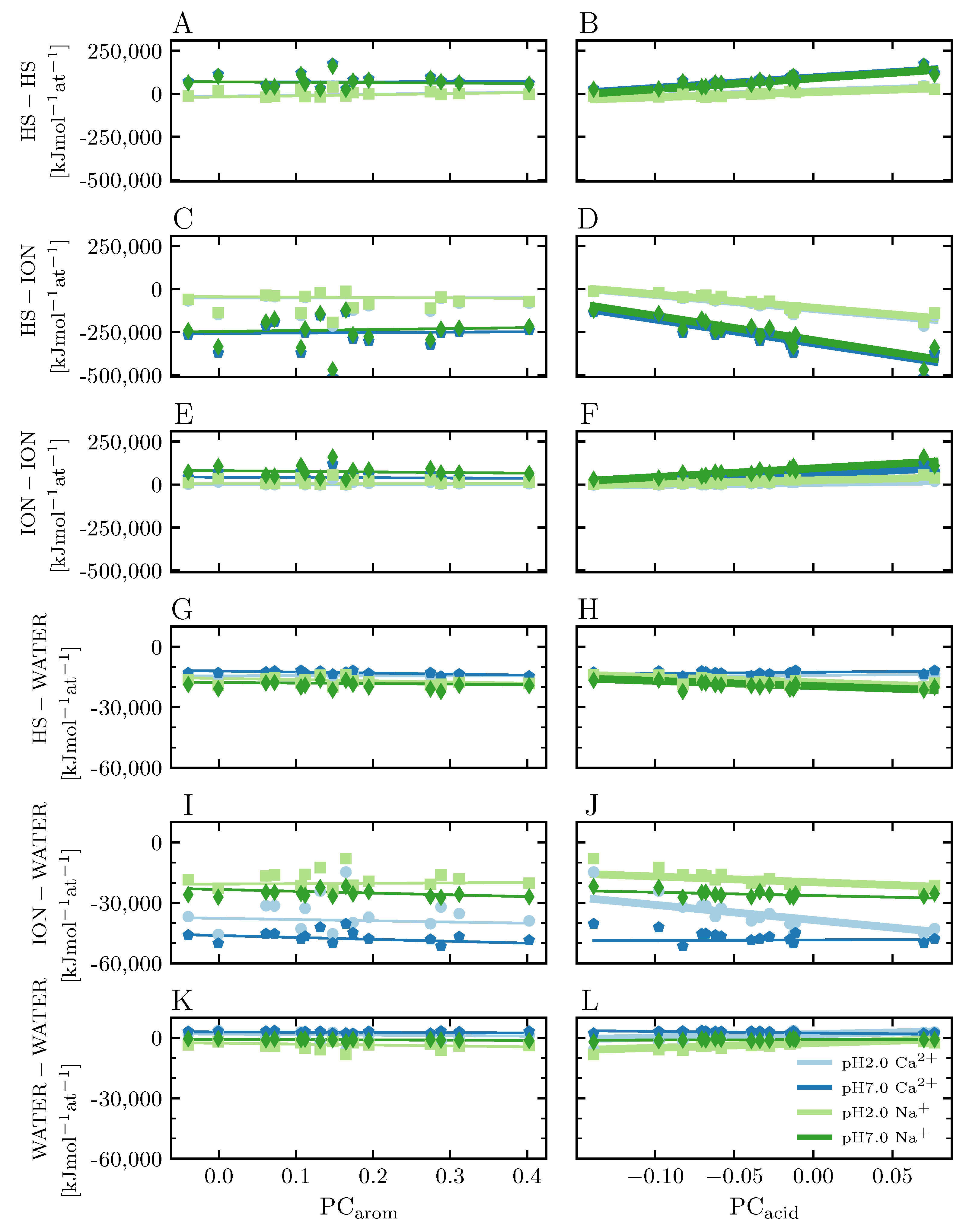
3.3.3. Nonbonded Interaction between Molecules

To gain insight into the nonbonded interactions between the humic substances, ions, and water in the system, we plotted the contribution by pairs of the molecules presented (see Figure 3). Results show that three pairs of interactions contribute primarily to the total potential energy.
These are the interactions within humic substances (see Figure 3A,B), the interactions between humic substances and ions (see Figure 3C,D), and the interactions between ions (see Figure 3E,F). From these three pairs, the one that contributes with the lowest values of potential energy is the interaction between humic substances and ions. As expected, the interaction between humic substances and ions is characterized principally by the presence of the inner complex structures formed between the carboxyl groups and cations [16]. With higher PC acid , the interaction between these two species becomes more favorable. This shows the relevance of this interaction for the whole stability of the system. In particular, because it counteracts the unfavorable interaction energies between humic substances (see Figure 3A,B) and between ionic species (see Figure 3E,F), due to repulsive coulombic interactions, which increase at higher PC acid composition.
As expected by our previous experiment, the PC acid content correlates with most of the energetic contributions of nonbonded interactions per pair of interactions. One exception is the interaction between humic substances and water (see Figure 3G,H) in the presence of calcium as counterion, indicating that calcium does not affect the interaction of these two species. Additionally, there are correlations with the PC acid and the energy between ion and water molecules at acidic pH (see Figure 3I,J), indicating that acidic systems, with more protonated carboxyl groups, indirectly affect the interactions between ions and water, possibly via hydrogen bonds, as suggested in our previous work [16].
Finally, the PC acid does not strongly affect the interaction between water molecules (see Figure 3K,L); just for sodium with neutral pH system, there is a tendency such that for high PC acid there is an increase in the nonbonded interaction between water molecules, indicating that the high concentration of sodium ions or carboxyl groups indirectly affects the interaction of water molecules, possibly due to the inclination of water molecules to solvate ionic species rather than making hydrogen bonds with other water molecules.

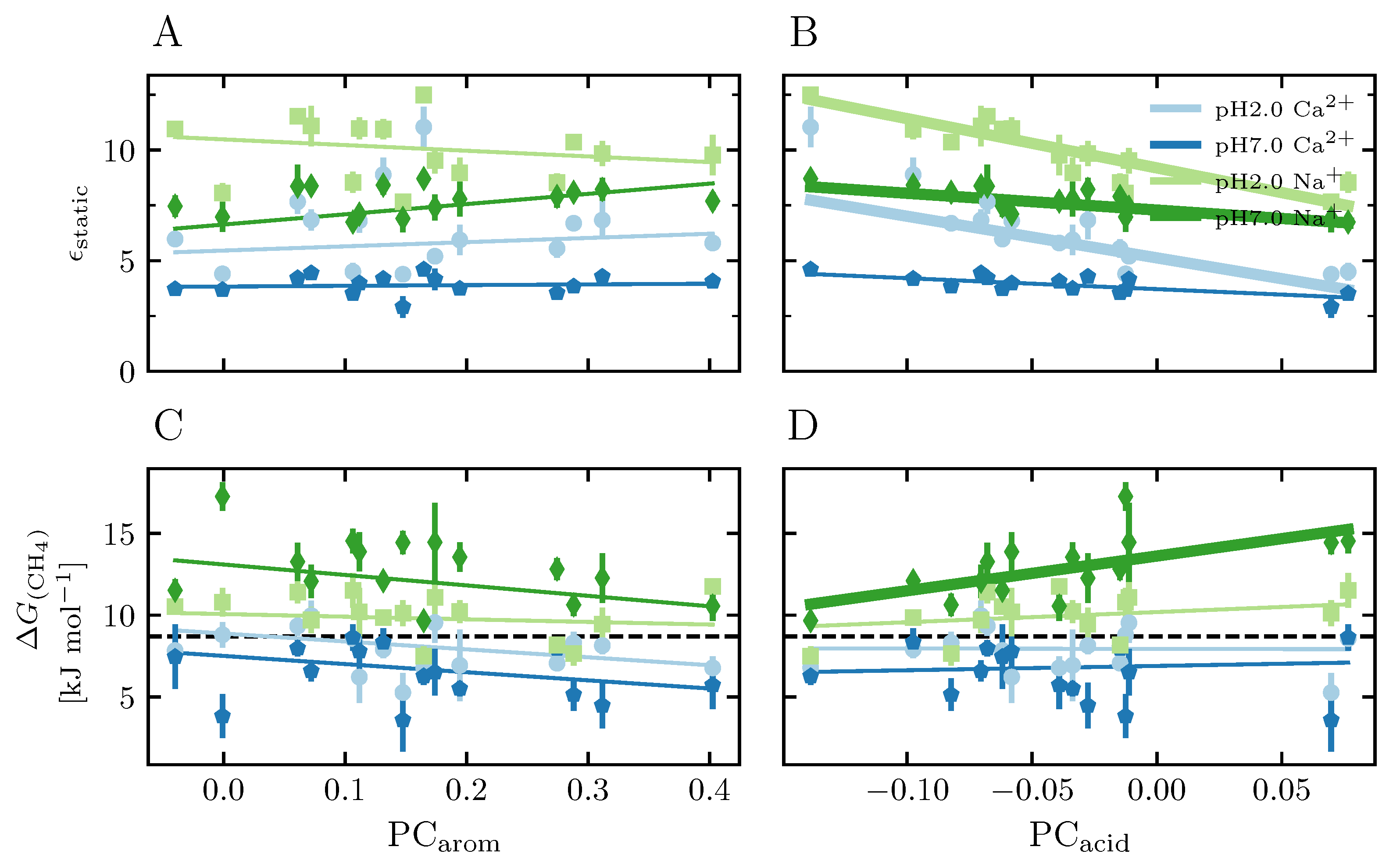
3.3.4. Static Relative Dielectric Constant

Considering the contribution of the charged species to the total potential energy, and to understand in more detail how the interaction of two point charges is affected by the chemical environment, we calculated the static relative dielectric constant, ϵ (see Figure 4A,B). Again, a correlation is observed between the static dielectric constant and the PC acid of the humic substances. The higher the PC acid , the lower the values of the dielectric constant. For systems containing calcium ions, the values of ϵ are lower than for the ones with sodium ions. This could be attributed to the interaction between cations and water molecules. Higher values of dielectric constant are associated with the rotation of water molecules due to polarization. This suggests that the systems with calcium have more restrictions in the movement of their molecules, especially water molecules, due to the presence of doubly charged species. The correlation seems stronger at low pH, suggesting that also an increase in protonated carboxylic acids restricts the motion of water molecules. In general, our results are in the range of experimental values that indicate that the dielectric permittivity, ϵ , of soils is between 2 and 20 for samples with soil moisture of 0 and 40% [29]. Related to a decrease in ϵ with an increase in PC acid , the dielectric constant of ionic solutions is known to reduce with an increasing ionic concentration because ions affect the polarization of solvent molecules [30].

3.3.5. Free Energy of Inserting a Methane Molecule

Another property related to the effect of charged species in the system is the free energy of inserting a methane molecule (see Figure 4C,D). This parameter permits us to identify the hydrophobicity of the modeled systems as a function of the PC arom and PC acid by inserting multiple times a methane molecule in random places of the whole system [31]. Interestingly, there is no correlation between the first PC (PC arom ) and the Δ G CH 4 of the insertion of a methane molecule for the different humic substances. However, there is a positive correlation with the PC acid of the humic substances, which indicates an unfavorable insertion of methane with higher PC acid . This phenomenon is observed in systems composed of sodium ions and neutral pH. It can be attributed to the high concentration of sodium ions in the system, which are with high PC acid , homogeneously distributed in the simulation box, which results in the insertion of a methane molecule to the system being more unfavorable. This could explain too why the systems with calcium ions have a lower value of Δ G CH 4 .

3.3.6. Diffusion

Dynamic properties are relevant to understanding how molecules interact with each other. Toward this aim, we calculated the self-diffusion coefficient, D of humic substances, ions and water, which permits us to understand their mobility individually (see Figure 5). The values were calculated using the slope between the mean-square displacement, Δ ( t ) , versus t for time intervals from 100 to 500 ps. This time range allows us to calculate the diffusion of atoms for which the movement is not restrained by the humic substance molecules.
The diffusion of the atoms of humic substance molecules (see Figure 5E,F) shows a reduced movement close to zero. Interestingly, the results show an apparent exponential decay of the diffusion of water molecules and ion species at low pH (see Figure 5B,D). Results indicate that at low pH, due to the presence of a major fraction of deprotonated/protonated carboxyl groups, cations and water molecules are free to move. This is supported by the fact that at higher PC acid , the diffusion decreases. Moreover, at a neutral pH, cations and water molecules have diffusion coefficients close to zero. This indicates their highly restricted movement in systems with high ionic species.

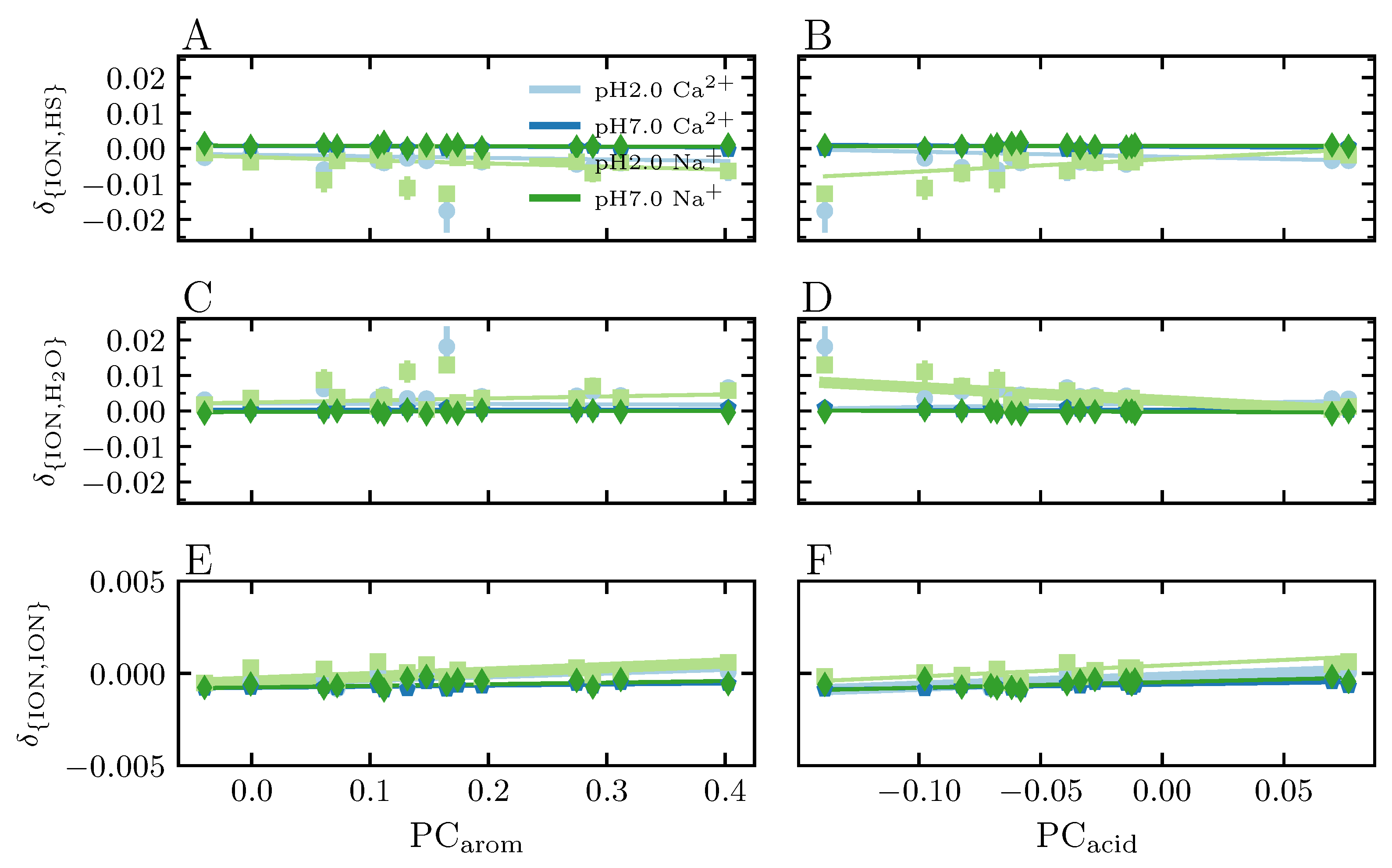
3.3.7. Preferential Solvation

We used the Kirkwood–Buff integrals to calculate the preferential solvation of humic substances (see Figure 6), water (see Figure 7), and ions (see Figure 8) separately. This permits us to gain insights into the molecular structure of our models. Positive values indicate preferential solvation, and negative values indicate a less favorable interaction between the species in question, while values close to zero are indicative of a heterogeneous solution.
We observe a correlation between PC acid and the preferential solvation of humic substances with themselves (positive) and with water molecules and ionic species (negative). Despite the correlations with the humic substance’s PC acid , the values of the preferential solvation do not change significantly for some of the studied systems.
However, we observe a negative preference for humic substances to be surrounded by other humic substances (see Figure 6B). This is more drastic in the case of systems containing sodium ion at an acidic pH. It can be attributed to the repulsion between humic substances due to the high content of carboxyl groups. Accordingly, the increasing carboxyl content of humic substances results in more favorable interaction with water molecules (see Figure 6D). Related to the cations, humic substances are preferably surrounded by sodium ions than calcium ions, which could be attributed to their amount in the systems. However, the PC acid (low pH) also demonstrates that the amount of deprotonated carboxyl groups also affects the preference of humic substances to be surrounded by cations.
Related to the preferential solvation of water molecules (see Figure 7), correlations in the preference of water molecules with humic substances and other water molecules in systems neutralized with sodium ions are observed. The preference to be solvated with humic substances is slightly negative for most of the cases, and clearly negative for the case of systems with sodium and at acidic pH (see Figure 7B). At low content of deprotonated carboxyl groups, water molecules prefer to interact with themselves (see Figure 7D).
In the case of preferential solvation of ions (see Figure 8), a correlation is observed only for a few cases with PC acid . Like the diffusion analysis, there is an exponential-decay-like function of the preference of ions with water molecules for systems with acidic systems (low pH) (see Figure 8D), which could be attributed to their interaction in the accessible cavities. This is accompanied by the low preference of ions to interact with humic substances (see Figure 8B). Cations are not preferentially solvated by themselves, an effect that becomes less pronounced with an increase in carboxyl content. Cation interactions are slightly unfavorable for low PC acid and in some conditions, this turns to be slightly favorable with PC acid (see Figure 8F).
Exploring the different combinations between two types of molecules from the set of HSs, water and ions, suggested that investigating even further the network of nonbonded interaction might be of great interest. For this reason, we calculated the number of hydrogen bonds and salt bridges presented in our systems.

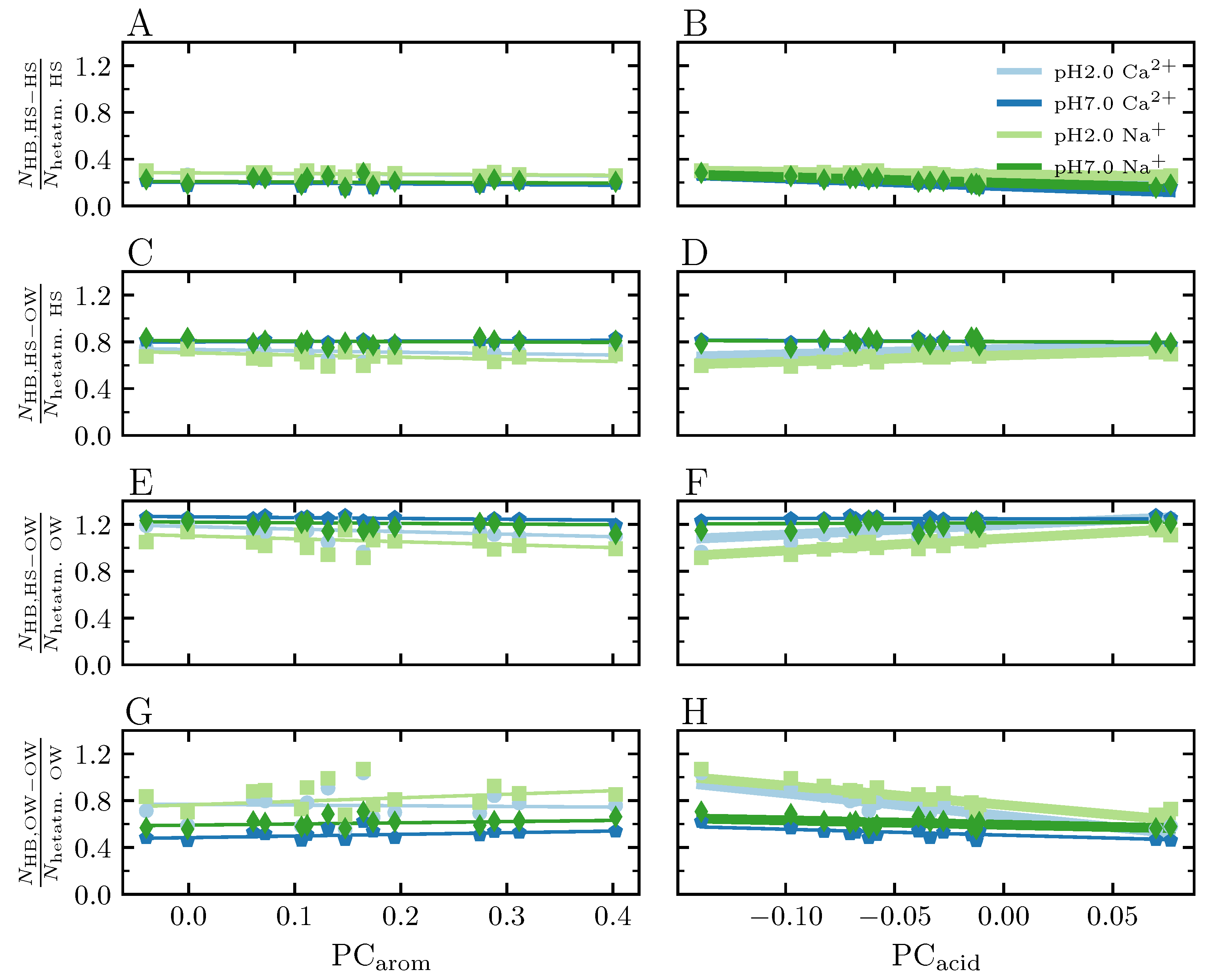
3.3.8. Hydrogen Bonds
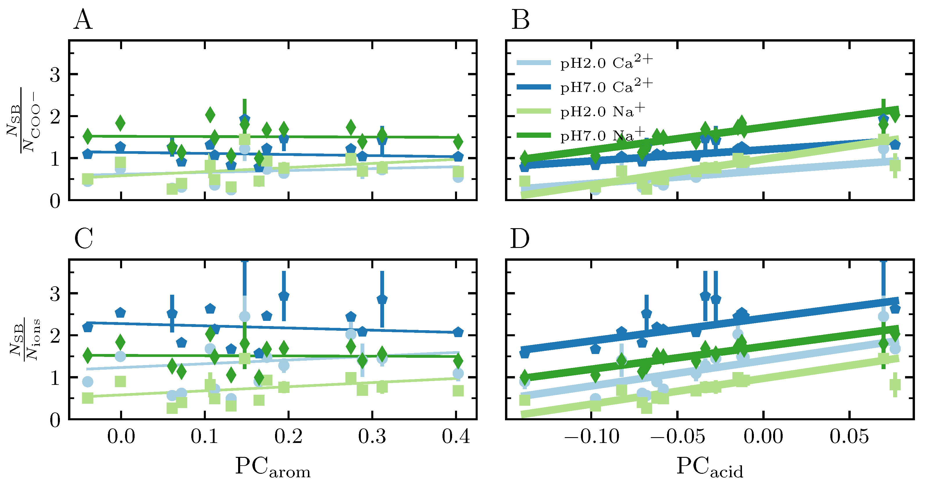
In order to understand the hydrogen bond network, we calculated the occurrence of hydrogen bonds between the humic substances and water molecules. Considering the differences in the number of functional groups between different models and also the difference between the number of water molecules to reach a certain water content, it was necessary to normalize the results by the number of heteroatoms of humic substances or water molecules ( N HB / N hetatm ), respectively (see Figure 9).
The result shows that the number of hydrogen bonds between humic substances normalized by the number of heteroatoms (see Figure 9A,B) is negatively correlated with the PC acid of the humic substances. This could be explained due to the high number of hydrogen bond acceptors but fewer donors in high deprotonated carboxyl groups.
The number of hydrogen bonds between humic substances and water molecules normalized by the number of heteroatoms of humic substances (see Figure 9C,D) do not show a correlation at neutral pH. However, at acidic pH, there is a positive correlation, which can be attributed to the increase in the protonated carboxylic groups.
The number of hydrogen bonds between humic substances and water molecules normalized by the number of heteroatoms of water molecules (see Figure 9E,F) shows similar results as the one normalized by humic substances.
In contrast, the number of hydrogen bonds between water molecules normalized by the number of heteroatoms (see Figure 9G,H) shows a negative correlation with PC acid . This indicates that low protonated carboxylic content permits water molecules to interact with each other, in agreement with a previous work [16]. Possibly due to their interaction in accessible cavities in these kinds of systems. These hydrogen bonds are reduced with high PC acid , indicating that the presence of an ionic species interferes with the interaction between water molecules.

3.3.9. Salt Bridges

Finally, with the aim of understanding in more detail the interactions between the carboxyl groups and the cations, we calculated the number of salt bridges observed in our simulations (see Figure 10). A salt bridge is considered to be any interaction between a carboxyl group and a counterion with a distance lower than 0.5 nm. We selected the ones that are maintained with occupancy above 90 percent of a simulation of 5 nanoseconds, indicating the stability and number of salt bridges per carboxyl groups or cations atoms.
The number of salt bridges between humic substances and cations normalized by the number of carboxyl groups of humic substances (see Figure 10A,B) show a correlation with the PC acid of the humic substances. This particular graph resembles the preferential solvation of humic substances by ions (see Figure 6F). However, this analysis adds more information about the connectivity of the carboxyl groups. For neutral and acidic pH, each deprotonated carboxyl group is able to interact closely with one cation and this value increases with the PC acid of the humic substances. Such an increase is also observed at low pH because of the high number of carboxyl groups.
The number of salt bridges between humic substances and cations normalized by the number of cations (see Figure 10C,D) shows information about the type of coordination of the cations. For neutral pH, calcium ions are able to coordinate two carboxyl groups up to three in the system with higher PC acid . For sodium ions, there is an increase in the coordination of carboxyl groups from one to two. This shows how strong the interaction between these charged species is, making the systems more stable, and supporting the previous analyses. In particular, trends in the total potential energy of the system (see Figure 2C,D), the contribution of nonbonded interaction between humic substances and cations, and the preferential solvation can be explained by this analysis.

4. Discussion

4.1. Humic Substances modeling

The atomistic modeling of soil organic matter, together with molecular dynamic simulation offers a computational microscope that allows us to understand the interactions of the soil organic compounds with their environment. In our case, its potential resides principally in the condensed-phase approach modeling of the soil organic matter. In the last decade, different studies have noticed the complexity of soil organic matter (SOM), in terms of composition as well as spatial disposition [1,32,33], making it essentially impossible to fully model SOM at an atomistic level at such time and length scales, which are orders of magnitude larger in comparison with the ones one we can address using molecular simulation. Therefore, different assumptions are needed to study SOM in terms of their atomistic interactions.
VSOMM2 creates simplistic models, which represent an average set of possible organic compounds presented in SOM. The validation of the models by computing spectroscopic properties [34,35,36] would be a powerful way to confirm the validity of the models. However, due to the complexity of the molecular systems, computing the vibrational or NMR spectra is not a simple undertaking. Furthermore, care must be taken that the compositional information from NMR experiments was directly used as input to create the models, excluding these properties from the validation experiment. Despite these shortcomings, we are confident that our models in combination with molecular dynamics permit us to predict macroscopically relevant properties of SOM. The use of an average set of molecules permits handling the complexity of molecules in a reduced physical space, which is necessary to reduce the computational requirements of larger systems with molecular dynamics.
Our previous studies were focused on the usage of the standard humic acid called leonardite (LHA), which corresponds to a sample obtained from the United States, enriched with high carbon content, representative of brown coal places. In particular, plain MD simulations allowed us to predict the physicochemical properties of LHA sample, which was in agreement with experimental data. Via free energy calculation, we were able to determine the absorption via molecular simulations and compare it with the experiment [18]. The Leonardite models also permitted us to understand the possible interaction with proteins [37] and clay minerals [38].
In this work, our aim is to improve our understanding of how composition and molecular interaction in SOM affect macroscopic properties. For this task, we modeled and simulated the current set of standard samples of humic substances provided by the International Humic Substances Society (IHSS). Despite the simplification of using extracted samples, the samples still present a heterogeneous organic composition, posing a challenge to the modeling. In order to compare the different macroscopic properties obtained from molecular simulation as a function of the humic substances, we created four independent models at two different pHs and with two different cations for each of the samples, leading to a total of 240 simulations (9.6 microseconds of simulation in total).

4.2. Organic Composition Analysis

The standardized humic substances come from four main sources: water, soil, peat, and leonardite. The IHSS also provides different analyses of the composition of the samples in their online platform. The main information, in terms of creating molecular models, is the 13 C NMR Carbon distribution, which gives insights into the functional groups present in the samples, in terms of the percentage of carbonyl, carboxyl, aromatic, acetal, heteroaliphatic, and aliphatic per humic substance [12].
In order to reduce the dimensionality of the organic compounds, a principal component analysis (PCA) was applied, which demonstrated that humic substances could be principally represented by their levels of aromaticity (PC arom ) and acidity (PC acid ), which are the first two principal components.
A previous PCA analysis by Schellekens et al. [39] of the humic substances resembled the importance of these two components, in their work denominated as aromaticity and solubility. The PCA, in this case, was determined in the process of comparing humic acids and fulvic acids by using Pyrolysis GC MS data. A direct comparison with our results remains difficult. However, our results using the organic composition of HS can determine similar principal components.
The first principal component, denominated aromaticity (PC arom ), shows that most of the humic substances are characterized by a positive value of PC arom , which is related to a high content of aromatic compounds and a low content of aliphatic compounds (see Figure A3), where, as expected, the HAs show, in general, higher PC arom in comparison with FAs due to the hydrophilic properties of the latter (see Figure 1). Compounds related with high PC arom are aromatic rings, which imply the composition of bulky hydrophobic compounds that interact with other hydrophobic compounds via van der Waals interaction and possibly promote the aggregation between organic compounds.
The second principal component, denominated as acidity (PC acid ), shows that humic substances vary in their composition. Positive values of PC acid indicate a high content of carboxyl and carbonyl groups. Meanwhile, negative values indicate the opposite (see Figure A3). The high content of carboxyl implies bulky compounds interacting with counterions and generating hydrogen bonds.
The mapping of the humic substances according to their principal components shows a dispersed pattern of points, where there is a tendency of high PC arom and low PC acid in humic acid in comparison to fulvic acids per sample. This is expected because HAs are by definition constituted of compounds with high molecular weight and low solubility at low pH, in comparison with FAs that are soluble at low pH.

4.3. Simulation Setup and Equilibration

In this work, we chose to create systems with a water content of 0.2 for all the systems, which corresponds to the value at which it is possible to obtain humic substances fully hydrated according to the previous studies of the Leonardite systems  [19].
In this work, we simulated the humic substances at pH 2.0 and at pH 7.0, which means that the carboxylic acids are on average 54 ± 13% and 0.2 ± 0.3% protonated, respectively. The systems were neutralized with sodium ions (according to the common experiments performed with NaOH [20]) or with calcium as a representative double charged ion. From a modeling side, our approximation uses a rough implementation of the protonation states, which considers only the protonation and deprotonation of carboxyl groups and the protonation of carboxyl groups is fixed during the simulation, and it does not depend on the environment of the functional group. This approximation permits simplistic simulations that can be easily simulated with current molecular dynamics simulation programs, such as GROMOS and GROMACS.
Due to the slow diffusion of molecules within the periodic box, especially the SOM molecules [17,19], systems need to be equilibrated using high temperatures for longer simulation times that permit overcoming the unfavorable position for humic substances, water and ions, in particular for the position between deprotonated carboxyl groups and cations, which contribute to the biggest forces in our systems. So, high temperature can assist to coordinate the positive ions with the closest carboxyl groups, minimizing the interaction energy [23]. In this work, with systems generated with a water content of 0.2, some systems were more difficult to equilibrate than others using the previous scheme. The reason for this behavior was the high carboxyl content of some of the studied samples. The carboxyl groups are relatively big in comparison with hydroxyl or carbonyl groups. More importantly, these groups are responsible for the ionic bonds with cations in the system contributing largely to the potential energy. Because their movements are restricted, the coordination with positive ions is even more difficult. For this reason, it was necessary to extend the simulation time at each of the temperatures to ensure a good equilibration.

4.4. Physical Properties of Modeled Humic Substances

With adequately equilibrated systems and production MD simulations, it is possible to estimate the macroscopic properties of modeled humic substances and compare the results to their composition. We performed a plethora of analyses to characterize the structure and dynamics of the systems. The systems depend on the level of carboxyl groups present in the system (level of PC a c i d ) and the counterions neutralizing those charges (Na + and CA 2 + ). In summary, three phenomena can be described. The first one is how the density and potential energy of the system is affected due to the closeness of charged species. The second is how the diffusion of water molecules affects the number of hydrogen bonds and dielectric constant of the systems. The third one is how the carboxyl groups affect the preferential solvation of the species and the network of salt bridges in the systems. These three properties are explained below and schematized in Figure 11.

4.4.1. Main Interactions in the System

As shown in Figure 11, the attractive interactions are between the carboxyl groups with the counterions, which counteract the repulsive interaction between carboxyl groups and between cations. These three pairs represent the stronger contribution to the total potential energy via Coulombic forces, where the close interaction between humic substances is a result of the Coulombic interactions between carboxyl groups and cations. There is a strong correlation such that the system size is affected by the number of carboxyl groups or PC acid . Between different counterions, there is a slightly high density in the calcium-containing system, possibly due to the salt bridge network. Galicia-Andrés et al. [16,38] suggest that higher densities are the result of the formation of bidentate structures, which are energetically more favorable.
The deprotonated carboxyl groups of humic acids interact with their counterions, which not only neutralize the negative charge of the humic acids but also reduce the electrostatic repulsion between them, a phenomenon called electrostatic stabilization [40].
In comparison with experimental data, in which densities range between 1300 and 1500 kg/m 3 for dried humic acid samples [41], our models show reasonable agreement. Considering that there is an increase in the density for models with lower water content [19], one could expect higher compactness close to or higher than 1600 kg/m 3 for fully dried humic substances with high PC acid .

4.4.2. Effect of Protonated Carboxyl Groups

The presence of high carboxyl content does not just permit a high level of compactness in the systems but also reduces the mobility of the molecules. At low or acid pH, the presence of protonated carboxyl groups permits a high movement of molecules, principally the water molecules, in comparison to when those carboxyl groups are deprotonated. Together with the analysis of the number of hydrogen bonds, results indicate high connectivity between water molecules via hydrogen bonds when carboxyl groups are in low content and protonated. This suggests that the deprotonated carboxyl groups are able to reduce the entropy of the system by stabilizing the water molecules via hydrogen bonds.
As proposed in previous works [14,16], the structure of humic substances is primarily driven by the cation-COO coordination in neutral pH conditions, and hydrogen bonding is important in low pH conditions.

4.4.3. Salt Bridges Network

Studies of the preferential solvation of humic substances with ionic species and the number of salt bridges in the systems demonstrate the presence of stable arrangements between carboxyl groups and cations. Remarkably, these analyses show new insights into the carboxyl–cation interaction. In agreement with previous works [16,42], we observed so-called cation bridges between carboxyl groups (COO ) and calcium. Furthermore, in this study, we quantified for systems neutralized with sodium ions and with high PC acid that carboxyl groups are able to coordinate two sodium ions, whereas for systems neutralized with calcium ions and with high PC acid , three calcium ions.
Sodium has a limited impact on the colloidal stability of SOM [43,44,45]. However, our results shed light on the role of monovalent ions in the presence of humic substances with high PC acid , where the interaction between sodium–carboxyl is the main contributor to the total potential energy of the humic substances.
When normalizing the number of salt bridges per cation number, we confirmed that cations can generate monodentate and bidentate coordination with carboxyl groups, as suggested in previous works [16,38,42,43,46]. As a whole, our experiments support the observations of Baalousha et al. [47], which indicated an increment in the humic substances network with increasing the calcium concentration, which is even more pronounced for neutral pH values.
This confirms that salt bridges confer the stability of the humic substances observed in the literature, demonstrating the importance of the cations for the macroscopic properties [14,16,42,43,45,46,48].

4.4.4. The Effect of the Aromaticity in the Studied Systems

Surprisingly, across different analyses performed in this study, there are only a few correlations observed with the PC arom of the humic substances. However, in the preference of ions with other ions, there is a correlation related to sodium ions, where PC arom plays an indirect role in the interaction of sodium. It seems that for high PC arom , there is a tendency for humic substances to interact with each other via hydrophobic interactions, excluding the presence of sodium ions. The high PC arom of humic substances relates to the close interaction between cations at an acidic pH. At low pH and low PC arom , as expected, the cations repel each other due to their equal charge sign. This phenomenon is not seen for calcium, and it could be attributed to the lower concentration (half) of ions in the system compared to sodium.

4.5. Extrapolation to Soil Organic Matter

Considering the humic substances as a model of soil organic matter, this suggests that soil oxidation leading to an increase in carboxyl species in soil organic compounds could promote more favorable structures in terms of their potential energy. In theory, Leonardite should present the lowest potential due to the characteristics of brown coal. However, the models are the result of experiments taken from alkaline extractions. Furthermore, for this particular case, the organic composition is determined by liquid state NMR, which has an intrinsic bias to observe soluble particles. In this regard, we should consider our humic substances models as de novo molecules that are potentially found in soil. In other words, the models could be considered as a representation of the solution-like molecules or gel-like molecules presented in the [1] model. The model from humic substances might be at odds with the real samples but present a great tool to gain insights into the structure, dynamics, and interactions within the soil organic matter. In particular, this study highlights the importance of the carboxyl–cation interaction, specifically how the carboxyl content and its protonation state content affect the macroscopic properties.
Unfortunately, due to the limitations of the molecular dynamics technique, it is difficult to estimate the macroscopic properties of this system with low water content, i.e., close to zero, in which we could speculate that the PC arom can play an important role, because molecules interact with each other strongly in the presence of different charged species and van der Waals interactions become dominant due to strong compaction. However, it is difficult to obtain equilibrated systems on dried models in terms of reaching an energetic local minimum just by arranging the molecules in a compacted way because the humic substances’ movement is slow.
Similarly, for high water content models, the formation of different phases may occur. The PC arom could be an intrinsic component in the formation of colloidal structures. This phenomenon has already been observed using the TNB model, assuming the formation of supramolecular structures, where hydrophilic and hydrophobic effects or cation–pi interactions may also influence the aggregation of humic acids [15].
In the current models, cations were added to neutralize the molecular systems, and their important role in bridging the interactions between SOM molecules was observed. However, the concentration of further inorganic ion species in real samples will have an additional effect on the interactions and dynamics of these molecules. Future work should involve a systematic study on the concentration effects of ions in the samples.
Furthermore, soil organic matter will rarely be observed as a single pure species, but interactions with other soil components lead to a complex matrix, consisting of soil minerals, organic matter, ionic species and water. The absorption of organic matter on clay minerals is a topic of ongoing research, to which molecular simulations will also contribute further [38].

5. Conclusions

The use of molecular dynamics simulations with models of humic substances can give us insights into several properties of soil organic matter as a function of their chemical composition. Our system permitted us to distinguish the properties of different humic substances, following the standardization created by the efforts of different researchers in the past, and shed light on the complexity of this unknown environment. Primarily, this study shows that the number of carboxyl groups and their interactions with cations, by and large, determine the overall behavior of the studied systems. Furthermore, the type of cations and pH further modify the properties, while the aromatic content of humic substances plays a surprisingly small role. Finally, this study exemplifies the power of MD simulations, which allows us to examine in detail the structure and dynamics of modeled systems, such as the formation of cavities, the interaction network of molecules presented in the system, and their mobility.

Author Contributions

Conceptualization, Y.E., D.P., E.G.-A. and C.O.; methodology, Y.E., D.P. and C.O.; software, Y.E.; validation, Y.E.; formal analysis, Y.E.; investigation, Y.E.; resources, C.O.; writing—original draft preparation, Y.E.; writing—review and editing, D.P., E.G.-A. and C.O.; visualization, Y.E.; supervision, D.P. and C.O.; project administration C.O., funding acquisition, D.P. and C.O. All authors have read and agreed to the published version of the manuscript.

Funding

This research was funded by the Austrian Science Fund (FWF) grant number 30224-N34.

Data Availability Statement

Data to generate the models can be obtained in https://somm.boku.ac.at/ accessed on 26 March 2023.

Acknowledgments

We acknowledge Open Access Funding by the Austrian Science Fund (FWF). We thank to Martin Gerzabek, Daniel Tunega and the MMS group for their help and fruitful discussions.

Conflicts of Interest

The authors declare no conflict of interest.

Abbreviations

    The following abbreviations are used in this manuscript:
HSHumic Substances
SOMSoil Organic Matter
HAHumic Acid
FAFulvic Acid
VSOMM2Vienna Soil Organic Matter Modeler 2

Appendix A

Appendix A.1. Principal Components Analysis (PCA) of Humic Substances

Besides studying the different humic substances models with the same water content, a problem arises, which consists of the way to correlate the observable macroscopic properties of our models with their chemical composition. We tried different approximations, such as grouping the data by their source type or between humic or fulvic acid. However, the broad spectrum of organic composition, even from the same source and extraction part, makes it difficult to classify using those terms. For this reason, we decided to study the organic composition using the principal components analysis, which will indicate the principal components from each model and how they could be reflected in the macroscopic properties.
We calculated the PCA for the organic composition parameters of humic substances using the Python module scikit-learn. The cumulative sum of the explained variance of the principal components shows that two components are able to represent more than 90% of the data (see Figure A2). The eigenvector of these two components was multiplied with the organic composition of the humic substances in order to classify each humic substance using two values. These values are associated with the aromaticity and acidity of the humic substances (see Figure A3). Therefore, in this work, the two first principal components are denominated PC arom and PC acid , respectively.

Appendix A.2. Humic Substances Models

VSOMM2 accepts as input the mass fraction of carbon and nitrogen and the composition fractions of the carbon distribution obtained from 13 C-NMR. We used the VSOMM2 modeler tool [23] to create four independent models of a set of standard humic substances provided by the International Humic Substances Society (IHSS) [12]. Each model contains 40 molecules, each composed of 5 building blocks. Therefore our models contain 200 building blocks in total per system, approximating the true diversity in humic substance samples. The pH of the system was set to neutral pH 7.0 and acidic pH 2.0, considering the pKa of carboxyl groups of each model as the one determined by titration experiments [49].
For each model, we created systems with different numbers of water molecules in order to satisfy a water content value of 0.2, which corresponds to the fraction of heavy atoms (all atoms, excluding hydrogens). After solvation, we neutralized the systems using sodium (Na + ) or calcium (Ca 2 + ) as a counterion (see Figure A1).
Figure A1. Exemplary representation of the molecular interactions of humic substances, calcium and water molecules. Humic substances are in black thick sticks, water molecules in space-filling representation, and calcium ions in green spheres.
Agronomy 13 01044 g0a1
Regarding the use of constant water content value, previously, in order to describe the structural and dynamic properties of humic substances, we generated different models with a different number of water molecules. This approximation was used to describe the great influence of the degree of solvation in the macroscopic properties of leonardite humic acid (LHA) models. However, due to the diversity between the current set of humic substances models, models contain a different number of atoms in order to accomplish the organic composition. For example, high carboxyl content requires carbon atoms associated with two oxygen atoms and one hydrogen atom; meanwhile, high aliphatic content models require just carbon atoms. Therefore, at the moment of solvation, models require a different number of water molecules to reach the same water content. For this reason, it was necessary to implement in VSOMM2 the use of water content as an input parameter instead of the number of water molecules, helping us in the process of comparison between different humic substances.

Appendix A.3. Humic Substances Simulations

After the minimization steps of VSOMM2, we tested different equilibration schemes that consisted of a series of molecular dynamics simulations at different temperatures (420 K, 360 K, and 300 K) following our previous results [19]. In this work, the systems were equilibrated using a scheme that corresponds to a simulation of 10 ns of equilibration at 420 K, followed by 10 ns at 360 K and then 15 ns at 300 K, using an initial density of 900 kg m 3 . All simulations were performed at a constant pressure of 1 bar.
Simulations were done at constant temperature and pressure, which were both maintained by weak coupling with a relaxation time of 0.1 ps and 2 ps, respectively [50]. The isothermal compressibility was estimated at 4.575 × 10 4 ( kJ mol 1 nm 3 ) 1 and pressure scaling was applied isotropically. We used a triple-range cutoff, where nonbonded interactions up to a short-range of 0.8 nm were calculated every 2 fs from a pair list that was updated every 10 fs. Interactions up to a long-range of 1.4 nm were calculated at pair-list updates and kept constant in between. For interactions beyond 1.4 nm, a reaction field contribution [51] with a dielectric constant of 61 [52] was included. The SHAKE algorithm was used to constrain bond lengths to their optimal values with a relative geometric accuracy of 10 4 [53]. This permits us to perform molecular dynamics simulations with a timestep of 2 fs. Production runs consist of 5 ns of simulation each, in which trajectory coordinates were collected every 0.2 ps for subsequent analysis.

Appendix A.4. Trajectory Analysis

The structure and dynamics of the simulated systems were analyzed using the gromos++ set of analysis programs [28]. The properties of each system were calculated as the average over four independent models, and statistical uncertainties were calculated as the standard error of the mean.

Appendix A.4.1. Density

The density ρ of the system was calculated as Kg m 3 .

Appendix A.4.2. Total Potential Energy

The potential energy E pot was normalized by the number of heavy atoms ( N HA ), denominated as E pot / N HA .

Appendix A.4.3. Nonbonded Interactions Between Molecules

We calculated the nonbonded interactions (Coulombic and van der Waals interactions) between humic substances molecules ( HS ), water molecules ( H 2 O ), and counterions ( Ca 2 + or Na + ).

Appendix A.4.4. Static Dielectric Constant

The static dielectric constant ( ϵ ) was calculated from the rotational part of the dipole moment [54]. The contribution of the translation part to the static dielectric constant was neglected because it represents less than 10% of the total value [17].

Appendix A.4.5. Free Energy of Inserting a Methane Molecule

We calculated the free energy of inserting a methane molecule into the humic substances models. This was calculated using the Widom particle insertion method [31] using 1000 insertion attempts every 0.2 ps of the simulation.

Appendix A.4.6. Diffusion Coefficient

To characterize the dynamics of the system, we calculated the diffusion coefficient, D, of the humic substances molecules ( D HS ), water molecules ( D water ), and counterions ( D Ca 2 + or D Na + ). First, we calculated the mean square-displacement ( Δ ( t ) ) of the center of mass of the whole molecules. We averaged over all considered molecules and over multiple time windows,
Δ ( t ) = 1 N a i = 1 N a ( r i ( t + τ ) r i ( τ ) ) 2 τ ,
where r i is the position of the atom i, N a is the number of atoms considered, and τ indicates the time origin. According to the Einstein relation, the diffusion constant was estimated using
D = lim t Δ ( t ) 6 t .

Appendix A.4.7. Preferential Solvation

The radial distribution function, g i j ( r ) , was calculated as
g i j ( r ) = n j ( r ) i , t 4 π r 2 d r ρ j ,
where n j ( r ) is the average number of j particles found in a bin centered at distance r from i particles, using a bin width of d r . ρ j is the density of j particles, obtained as the total number of j particles divided by the simulation box volume.
Kirkwood–Buff integrals ( G i j ) were calculated using the radial distribution functions and using a correction parameter determined by Krüger et al. [55] as
G i j ( R ) = 0 R 2 π r 2 ω ( r ) ( g ( r ) 1 ) d r ,
where g ( r ) is the radial distribution function, R is the upper boundary of 1.5 nm, and ω ( r ) is the correction factor defined as
ω ( r ) = 1 r R 3 .
The preferential solvation of species j around species i is calculated as
δ i , j = x j G i , j α x α G i , α V corr + α x α G i , α ,
where α x α G i , α correspond to the summation of the Kirkwood–Buff between the species i with the species α , which corresponds to itself and others species multiplied by the molar fraction of the specie α . V corr is the correction volume: 4 / 3 π R 3 . Molar fractions are calculated as the normalized number of heavy atoms (no-hydrogens).

Appendix A.4.8. Number of Hydrogen Bonds

For a better understanding of the interactions between the humic substances and water, we monitored the hydrogen bonds normalized by the number of hetero atoms as follows: between humic substances molecules (HS–HS) and between HS and water (HS–water) the number of hydrogen bonds is normalized by the number of heteroatoms ( N hetatm ) of humic substances. Between HS and water (HS–water) and water molecules (water–water), the number of hydrogen bonds is normalized by the number of heteroatoms of water molecules, which correspond to the total number of water molecules.

Appendix A.4.9. Number of Salt Bridges

For a better understanding of the interactions between the humic substances and cations, we monitored the number of salt bridges (N SB ) normalized by the number of carboxyl groups or the number of cations. A salt bridge was defined as any interaction with a distance lower than 0.5 nm between a carboxyl group and a cation which is maintained at least at 90% of a simulation time of 5 ns.

Appendix B. Figures

Figure A2. The cumulative sum of the explained variance of the principal components.
Agronomy 13 01044 g0a2
Figure A3. Correlation of the principal components PC arom and PC acid with the organic composition of the humic substances. Each plot has a fitted line using linear regression, which is presented with a green tick curve if the R 2 is greater than 0.6.
Agronomy 13 01044 g0a3

References

  1. Masoom, H.; Courtier-Murias, D.; Farooq, H.; Soong, R.; Kelleher, B.P.; Zhang, C.; Maas, W.E.; Fey, M.; Kumar, R.; Monette, M.; et al. Soil Organic Matter in Its Native State: Unravelling the Most Complex Biomaterial on Earth. Environ. Sci. Technol. 2016, 50, 1670–1680. [Google Scholar] [CrossRef] [PubMed]
  2. Paul, E.A. The nature and dynamics of soil organic matter: Plant inputs, microbial transformations, and organic matter stabilization. Soil Biol. Biochem. 2016, 98, 109–126. [Google Scholar] [CrossRef] [Green Version]
  3. Chen, X.D.; Dunfield, K.E.; Fraser, T.D.; Wakelin, S.A.; Richardson, A.E.; Condron, L.M. Soil biodiversity and biogeochemical function in managed ecosystems. Soil Res. 2020, 58, 1–20. [Google Scholar] [CrossRef] [Green Version]
  4. Zhang, Y.; Liu, X.; Zhang, C.; Lu, X. A combined first principles and classical molecular dynamics study of clay-soil organic matters (SOMs) interactions. Geochim. Cosmochim. Acta 2020, 291, 110–125. [Google Scholar] [CrossRef]
  5. Kibblewhite, M.G.; Ritz, K.; Swift, M.J. Soil health in agricultural systems. Philos. Trans. R. Soc. Biol. Sci. 2008, 363, 685–701. [Google Scholar] [CrossRef] [PubMed] [Green Version]
  6. Bui, M.; Adjiman, C.S.; Bardow, A.; Anthony, E.J.; Boston, A.; Brown, S.; Fennell, P.S.; Fuss, S.; Galindo, A.; Hackett, L.A.; et al. Carbon capture and storage (CCS): The way forward. Energy Environ. Sci. 2018, 11, 1062–1176. [Google Scholar] [CrossRef] [Green Version]
  7. Wiesmeier, M.; Urbanski, L.; Hobley, E.; Lang, B.; von Lützow, M.; Marin-Spiotta, E.; van Wesemael, B.; Rabot, E.; Ließ, M.; Garcia-Franco, N.; et al. Soil organic carbon storage as a key function of soils - A review of drivers and indicators at various scales. Geoderma 2019, 333, 149–162. [Google Scholar] [CrossRef]
  8. Rabot, E.; Wiesmeier, M.; Schlüter, S.; Vogel, H.J. Soil structure as an indicator of soil functions: A review. Geoderma 2018, 314, 122–137. [Google Scholar] [CrossRef]
  9. Hayes, M.H.; Swift, R.S. Vindication of Humic Substances as a Key Component of Organic Matter in Soil and Water, 1st ed.; Elsevier: Amsterdam, The Netherlands, 2020; Volume 163, pp. 1–37. [Google Scholar] [CrossRef]
  10. Kögel-Knabner, I.; Rumpel, C. Advances in Molecular Approaches for Understanding Soil Organic Matter Composition, Origin, and Turnover: A Historical Overview, 1st ed.; Elsevier: Amsterdam, The Netherlands, 2018; Volume 149, pp. 1–48. [Google Scholar] [CrossRef]
  11. Kleber, M.; Johnson, M.G. Advances in Understanding the Molecular Structure of Soil Organic Matter, 1st ed.; Elsevier: Amsterdam, The Netherlands, 2010; Volume 106, pp. 77–142. [Google Scholar] [CrossRef]
  12. IHSS. 2020. Available online: http://humic-substances.org/ (accessed on 26 March 2023).
  13. Tuckerman, M.E. Statistical Mechanics: Theory and Molecular Simulation, 1st ed.; Oxford University Press: Oxford, UK, 2010; pp. 95–96. [Google Scholar]
  14. Ai, Y.; Zhao, C.; Sun, L.; Wang, X.; Liang, L. Coagulation mechanisms of humic acid in metal ions solution under different pH conditions: A molecular dynamics simulation. Sci. Total Environ. 2020, 702, 135072. [Google Scholar] [CrossRef]
  15. Tan, L.; Yu, Z.; Tan, X.; Fang, M.; Wang, X.; Wang, J.; Xing, J.; Ai, Y.; Wang, X. Systematic studies on the binding of metal ions in aggregates of humic acid: Aggregation kinetics, spectroscopic analyses and MD simulations. Environ. Pollut. 2019, 246, 999–1007. [Google Scholar] [CrossRef]
  16. Galicia-Andrés, E.; Escalona, Y.; Oostenbrink, C.; Tunega, D.; Gerzabek, M.H. Soil organic matter stabilization at molecular scale: The role of metal cations and hydrogen bonds. Geoderma 2021, 401, 115237. [Google Scholar] [CrossRef]
  17. Petrov, D.; Tunega, D.; Gerzabek, M.H.; Oostenbrink, C. Molecular Dynamics Simulations of the Standard Leonardite Humic Acid: Microscopic Analysis of the Structure and Dynamics. Environ. Sci. Technol. 2017, 51, 5414–5424. [Google Scholar] [CrossRef]
  18. Petrov, D.; Tunega, D.; Gerzabek, M.H.; Oostenbrink, C. Molecular modelling of sorption processes of a range of diverse small organic molecules in Leonardite humic acid. Eur. J. Soil Sci. 2020, 71, 831–844. [Google Scholar] [CrossRef] [PubMed] [Green Version]
  19. Escalona, Y.; Petrov, D.; Oostenbrink, C. Modeling soil organic matter: Changes in macroscopic properties due to microscopic changes. Geochim. Cosmochim. Acta 2021, 307, 228–241. [Google Scholar] [CrossRef]
  20. Thorn, K.A.; Folan, D.W.; MacCarthy, P. Characterization of the International Humic Substances Society Standard and Reference Fulvic and Humic Acids by Solution State Carbon-13 (13C) and Hydrogen-1 (1H) Nuclear Magnetic Resonance Spectrometry; Water-Resources Investigations Report 89-4196 (USGS); U.S. Geological Survey: Reston, VA, USA, 1989; Volume 13, p. 99.
  21. Niederer, C.; Goss, K.U.; Schwarzenbach, R.P. Sorption equilibrium of a wide spectrum of organic vapors in leonardite humic acid: Modeling of experimental data. Environ. Sci. Technol. 2006, 40, 5374–5379. [Google Scholar] [CrossRef]
  22. Escalona Balboa, Y.I. Towards The Understanding of Soil Organic Matter via Molecular Modeling and Simulations. 2021. Available online: https://permalink.obvsg.at/bok/AC16438986 (accessed on 26 March 2023).
  23. Escalona, Y.; Petrov, D.; Oostenbrink, C. Vienna soil organic matter modeler 2 (VSOMM2). J. Mol. Graph. Model. 2021, 103, 107817. [Google Scholar] [CrossRef]
  24. Schmid, N.; Eichenberger, A.P.; Choutko, A.; Riniker, S.; Winger, M.; Mark, A.E.; Van Gunsteren, W.F. Definition and testing of the GROMOS force-field versions 54A7 and 54B7. Eur. Biophys. J. 2011, 40, 843–856. [Google Scholar] [CrossRef]
  25. Schmid, N.; Christ, C.D.; Christen, M.; Eichenberger, A.P.; Van Gunsteren, W.F. Architecture, implementation and parallelisation of the GROMOS software for biomolecular simulation. Comput. Phys. Commun. 2012, 183, 890–903. [Google Scholar] [CrossRef]
  26. Oostenbrink, C.; Villa, A.; Mark, A.E.; Van Gunsteren, W.F. A biomolecular force field based on the free enthalpy of hydration and solvation: The GROMOS force-field parameter sets 53A5 and 53A6. J. Comput. Chem. 2004, 25, 1656–1676. [Google Scholar] [CrossRef]
  27. Reif, M.M.; Hünenberger, P.H.; Oostenbrink, C. New interaction parameters for charged amino acid side chains in the GROMOS force field. J. Chem. Theory Comput. 2012, 8, 3705–3723. [Google Scholar] [CrossRef]
  28. Eichenberger, A.P.; Allison, J.R.; Dolenc, J.; Geerke, D.P.; Horta, B.A.C.; Meier, K.; Oostenbrink, C.; Schmid, N.; Steiner, D.; Wang, D.; et al. GROMOS++ software for the analysis of biomolecular simulation trajectories. J. Chem. Theory Comput. 2011, 7, 3379–3390. [Google Scholar] [CrossRef] [PubMed]
  29. Demontoux, F.; Le Crom, B.; Ruffié, G.; Wigneron, J.P.; Grant, J.P.; Mironov, V.L.; Lawrence, H. Electromagnetic characterization of soil-litter media: Application to the simulation of the microwave emissivity of the ground surface in forests. Eur. Phys. J. Appl. Phys. 2008, 44, 303–315. [Google Scholar] [CrossRef]
  30. Adar, R.M.; Markovich, T.; Levy, A.; Orland, H.; Andelman, D. Dielectric constant of ionic solutions: Combined effects of correlations and excluded volume. J. Chem. Phys. 2018, 149, 1–10. [Google Scholar] [CrossRef] [PubMed] [Green Version]
  31. Widom, B. Some Topics in the Theory of Fluids. J. Chem. Phys. 1963, 39, 2808–2812. [Google Scholar] [CrossRef]
  32. Lehmann, J.; Solomon, D.; Kinyangi, J.; Dathe, L.; Wirick, S.; Jacobsen, C. Spatial complexity of soil organic matter forms at nanometre scales. Nat. Geosci. 2008, 1, 238–242. [Google Scholar] [CrossRef]
  33. Piccolo, A.; Spaccini, R.; Savy, D.; Drosos, M. The Soil Humeome: Chemical Structure, Functions and Technological Perspectives. In Sustainable Agrochemistry; Springer: Berlin/Heidelberg, Germany, 2019. [Google Scholar] [CrossRef]
  34. Trout, C.C.; Kubicki, J.D. UV Resonance Raman Spectra and Molecular Orbital Calculations of Salicylic and Phthalic Acids Complexed to Al3+ in Solution and on Mineral Surfaces. J. Phys. Chem. A 2004, 108, 11580–11590. [Google Scholar] [CrossRef]
  35. Watts, H.D.; Mohamed, M.N.A.; Kubicki, J.D. Comparison of Multistandard and TMS-Standard Calculated NMR Shifts for Coniferyl Alcohol and Application of the Multistandard Method to Lignin Dimers. J. Phys. Chem. B 2011, 115, 1958–1970. [Google Scholar] [CrossRef]
  36. Trout, C.C.; Tambach, T.; Kubicki, J.D. Correlation of observed and model vibrational frequencies for aqueous organic acids: UV resonance Raman spectra and molecular orbital calculations of benzoic, salicylic, and phthalic acids. Spectrochim. Acta Part Mol. Biomol. Spectrosc. 2005, 61, 2622–2633. [Google Scholar] [CrossRef]
  37. Gotsmy, M.; Escalona, Y.; Oostenbrink, C.; Petrov, D. Exploring the structure and dynamics of proteins in soil organic matter. Proteins Struct. Funct. Bioinform. 2021, 89, 925–936. [Google Scholar] [CrossRef]
  38. Galicia-Andrés, E.; Oostenbrink, C.; Gerzabek, M.H.; Tunega, D. On the Adsorption Mechanism of Humic Substances on Kaolinite and Their Microscopic Structure. Minerals 2021, 11, 1138. [Google Scholar] [CrossRef]
  39. Schellekens, J.; Buurman, P.; Kalbitz, K.; Zomeren, A.V.; Vidal-Torrado, P.; Cerli, C.; Comans, R.N. Molecular Features of Humic Acids and Fulvic Acids from Contrasting Environments. Environ. Sci. Technol. 2017, 51, 1330–1339. [Google Scholar] [CrossRef] [PubMed] [Green Version]
  40. Chen, K.L.; Smith, B.A.; Ball, W.P.; Fairbrother, D.H. Assessing the colloidal properties of engineered nanoparticles in water: Case studies from fullerene C60 nanoparticles and carbon nanotubes. Environ. Chem. 2010, 7, 10–27. [Google Scholar] [CrossRef] [Green Version]
  41. Tatzber, M.; Stemmer, M.; Spiegel, H.; Katzlberger, C.; Haberhauer, G.; Gerzabek, M.H. Impact of different tillage practices on molecular characteristics of humic acids in a long-term field experiment - An application of three different spectroscopic methods. Sci. Total Environ. 2008, 406, 256–268. [Google Scholar] [CrossRef] [PubMed]
  42. Kalinichev, A.G.; Iskrenova-Tchoukova, E.; Ahn, W.Y.; Clark, M.M.; Kirkpatrick, R.J. Effects of Ca2+ on supramolecular aggregation of natural organic matter in aqueous solutions: A comparison of molecular modeling approaches. Geoderma 2011, 169, 27–32. [Google Scholar] [CrossRef] [Green Version]
  43. Iskrenova-Tchoukova, E.; Kalinichev, A.G.; Kirkpatrick, R.J. Metal Cation Complexation with Natural Organic Matter in Aqueous Solutions: Molecular Dynamics Simulations and Potentials of Mean Force. Langmuir 2010, 26, 15909–15919. [Google Scholar] [CrossRef] [Green Version]
  44. Xu, F.; Wei, C.; Zeng, Q.; Li, X.; Alvarez, P.J.; Li, Q.; Qu, X.; Zhu, D. Aggregation Behavior of Dissolved Black Carbon: Implications for Vertical Mass Flux and Fractionation in Aquatic Systems. Environ. Sci. Technol. 2017, 51, 13723–13732. [Google Scholar] [CrossRef]
  45. Wei, P.; Xu, F.; Fu, H.; Qu, X. Impact of origin and structure on the aggregation behavior of natural organic matter. Chemosphere 2020, 248, 125990. [Google Scholar] [CrossRef]
  46. Kalinichev, A.G.; Kirkpatrick, R.J. Molecular dynamics simulation of cationic complexation with natural organic matter. Eur. J. Soil Sci. 2007, 58, 909–917. [Google Scholar] [CrossRef]
  47. Baalousha, M.; Motelica-Heino, M.; Coustumer, P.L. Conformation and size of humic substances: Effects of major cation concentration and type, pH, salinity, and residence time. Colloids Surfaces Physicochem. Eng. Asp. 2006, 272, 48–55. [Google Scholar] [CrossRef]
  48. Aquino, A.J.; Tunega, D.; Schaumann, G.E.; Haberhauer, G.; Gerzabek, M.H.; Lischka, H. The functionality of cation bridges for binding polar groups in soil aggregates. Int. J. Quantum Chem. 2011, 111, 1531–1542. [Google Scholar] [CrossRef]
  49. Ritchie, J.D.; Michael Perdue, E. Proton-binding study of standard and reference fulvic acids, humic acids, and natural organic matter. Geochim. Cosmochim. Acta 2003, 67, 85–96. [Google Scholar] [CrossRef]
  50. Berendsen, H.J.; Postma, J.P.; Van Gunsteren, W.F.; Dinola, A.; Haak, J.R. Molecular dynamics with coupling to an external bath. J. Chem. Phys. 1984, 81, 3684–3690. [Google Scholar] [CrossRef] [Green Version]
  51. Tironi, I.G.; Sperb, R.; Smith, P.E.; Van Gunsteren, W.F. A generalized reaction field method for molecular dynamics simulations. J. Chem. Phys. 1995, 102, 5451–5459. [Google Scholar] [CrossRef]
  52. Heinz, T.N.; Van Gunsteren, W.F.; Hünenberger, P.H. Comparison of four methods to compute the dielectric permittivity of liquids from molecular dynamics simulations. J. Chem. Phys. 2001, 115, 1125–1136. [Google Scholar] [CrossRef]
  53. Ryckaert, J.P.; Ciccotti, G.; Berendsen, H.J. Numerical integration of the cartesian equations of motion of a system with constraints: Molecular dynamics of n-alkanes. J. Comput. Phys. 1977, 23, 327–341. [Google Scholar] [CrossRef] [Green Version]
  54. Schröder, C.; Steinhauser, O. Using fit functions in computational dielectric spectroscopy. J. Chem. Phys. 2010, 132, 244109. [Google Scholar] [CrossRef]
  55. Krüger, P.; Schnell, S.K.; Bedeaux, D.; Kjelstrup, S.; Vlugt, T.J.H.; Simon, J.M. Kirkwood-Buff integrals for finite volumes. J. Phys. Chem. Lett. 2013, 4, 235–238. [Google Scholar] [CrossRef]
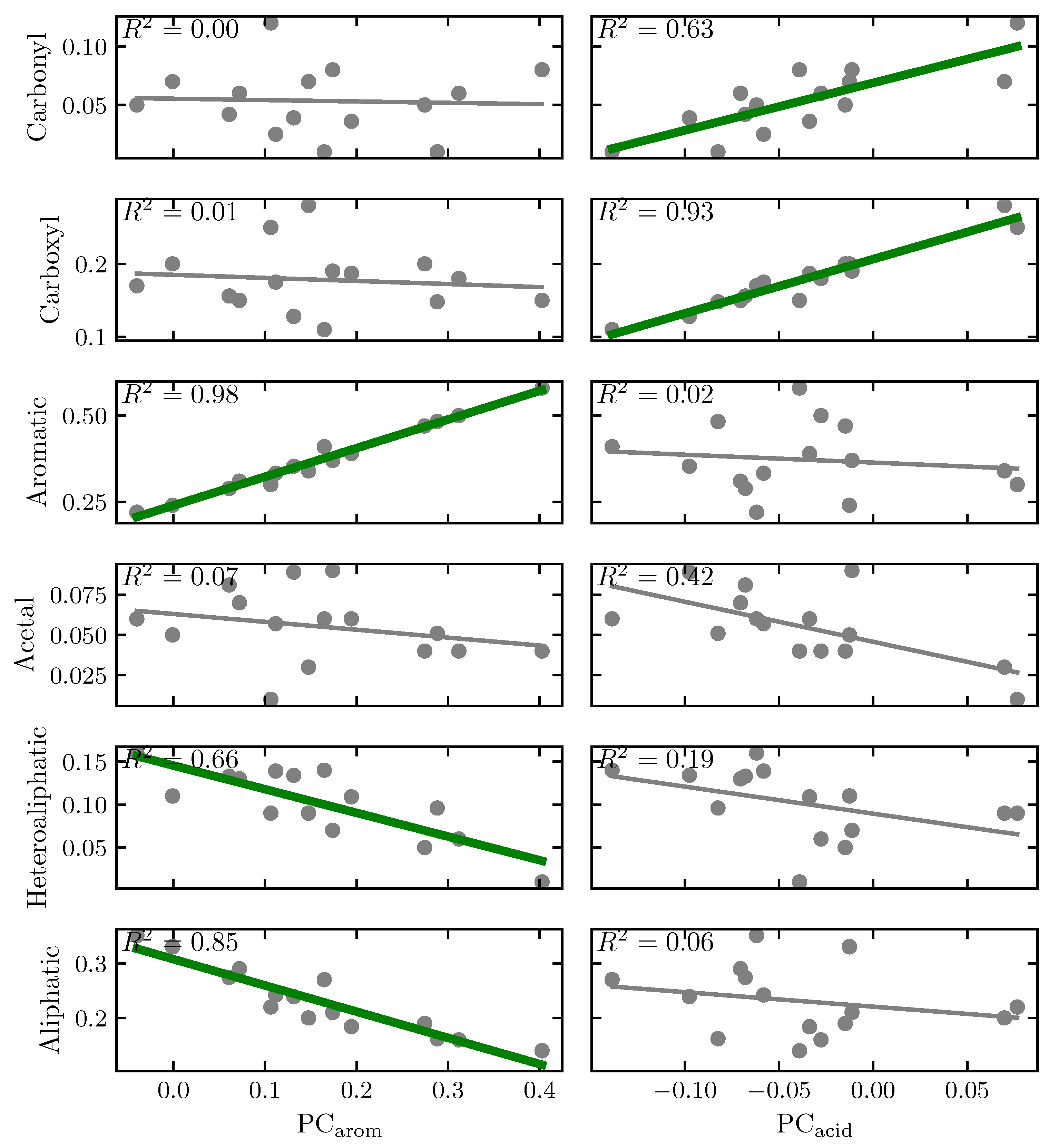
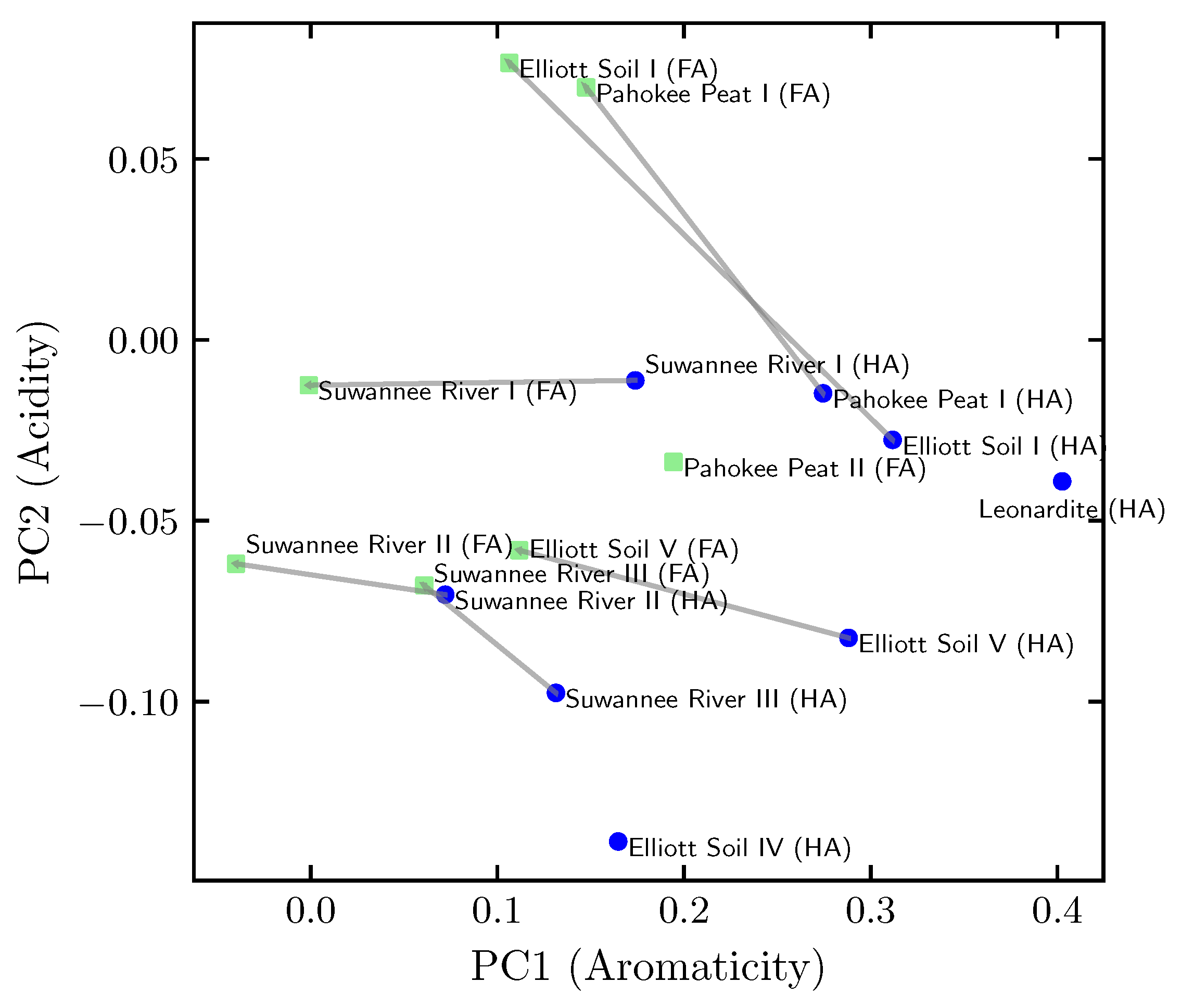
Figure 1. Principal component analysis of the humic substances according to their organic composition. Each point represents a different sample of HS. Blue circles represent humic acids; meanwhile, green squares represent fulvic acids. Arrows connect humic substances extracted from the same source.
Agronomy 13 01044 g001
Figure 2. Properties of the standard humic substances as a function of the first two principal components. Each point represents the average over four independent simulations with error bars representing the standard error. Each plot has a fitted line using linear regression, which is presented with a tick curve if the R 2 is greater than 0.6. (A,B) Density and (C,D) Total potential energy of the system normalized by the number of heavy atoms as a function of the PC arom and PC acid of the humic substances.
Agronomy 13 01044 g002
Figure 3. Nonbonded interaction between different species (HS, H 2 O and Ca 2 + ) of the standard humic substances models. (A,B) Nonbonded interactions between humic substances. (C,D) Nonbonded interactions between humic substances and cations. (E,F) Nonbonded interactions between cations. (G,H) Nonbonded interactions between humic substances and water molecules. (I,J) Nonbonded interactions between cations and water molecules. (K,L) Nonbonded interactions between water molecules. Each point represents the average over four independent simulations, with error bars representing the standard error. Each plot has fitted lines using weighted linear regression, which are presented as a tick line if the R 2 is larger than 0.6. Notice the different y-axis scales in these plots.
Agronomy 13 01044 g003
Figure 4. Static relative dielectric constant and free energy of inserting a methane molecule of the standard humic substances as a function of the principal components. Each point represents the average over four independent simulations with error bars representing the standard error. Each plot has a fitted line using linear regression, which is presented as a tick line if the R 2 is larger than 0.6. (A,B) dielectric constant and (C,D) free energy of inserting a methane probe into different humic substances models as a function of their PC arom and PC acid .
Agronomy 13 01044 g004
Figure 5. Diffusion of the standard humic substances models as a function of their PC arom and PC acid . Plots show the diffusion of water molecules (A,B), cations (C,D) and humic substances (E,F) in function of their PC arom and PC acid . Each point represents the average over four independent simulations with error bars representing the standard error. Notice the different y-axis scales in these plots.
Agronomy 13 01044 g005
Figure 6. Preferential solvation of humic substances with different species (HS, H 2 O and Ca 2 + ) of the standard humic substances models. Plots show the preferential solvation with (A,B) the humic substances, (C,D) water and (E,F) cations (calcium or sodium) in function of their PC arom and PC acid . Each point represents the average over four independent simulations with error bars representing the standard error. Notice the different y-axis scales in these plots.
Agronomy 13 01044 g006
Figure 7. Preferential solvation of water molecules with different species (HS, H 2 O and Ca 2 + ) of the standard humic substances models. Plots show the preferential solvation with (A,B) the humic substances, (C,D) water and (E,F) cations (calcium or sodium) in function of their PC arom and PC acid . Each point represents the average over four independent simulations with error bars representing the standard error. Notice the different y-axis scales in these plots.
Agronomy 13 01044 g007
Figure 8. Preferential solvation of cations with different species (HS, H 2 O and Ca 2 + ) of the standard humic substances models. Plots show the preferential solvation with (A,B) the humic substances, (C,D) water and (E,F) cations (calcium or sodium) in function of their PC arom and PC acid . Each point represents the average over four independent simulations with error bars representing the standard error. Notice the different y-axis scales in our plots.
Agronomy 13 01044 g008
Figure 9. Number of hydrogen bonds of the humic substances models normalized by the number of heteroatoms as a function of their PC arom and PC acid . Number of hydrogen bonds between humic substances normalized by the number of heteroatoms of humic substances (A,B). Number of hydrogen bonds between humic substances and water molecules normalized by the number of heteroatoms of humic substances (C,D) and normalized by the number of heteroatoms of water molecules (same as the number of water molecules) (E,F). Number of hydrogen bonds between water molecules normalized by the number of water molecules (G,H). Each point represents the average over four independent simulations with error bars representing the standard error.
Agronomy 13 01044 g009
Figure 10. Number of salt bridges (N SB ) of the humic substances models as a function of their PC arom and PC acid . Number of salt bridges (N SB ) of the humic substances models normalized by the number of carboxyl groups (N COO ) (A,B). Number of salt bridges (N SB ) of the humic substances models normalized by the number of ions (N ions ) (C,D). Each point represents the average over four independent simulations with error bars representing the standard error.
Agronomy 13 01044 g010
Figure 11. Schematic summary of the main properties of the system depend on the low and high levels of PC a c i d and the counterions Na + and CA 2 + . Each system contains three parts. The first (top left) describes the pair of interactions that contributes largely to the potential energy of the system (carboxyl groups of HS, carboxyl group of HS with counterion, and the interaction between cations). The second (top right) describes the interaction of water molecules with protonated carboxyl groups of HS. The third (down, center) is the presence of salt bridges and ways of interaction between carboxyl groups and counterions.
Agronomy 13 01044 g011
Table 1. Summary of the characteristics of the first two principal components (PC arom and PC acid ).
NegativePositive
PC arom high hetero- & aliphatic contenthigh aromatic content
e.g., Suwannee River II (FA)e.g., Leonardite (HA)
PC acid low carboxyl and carbonyl contenthigh carboxyl and carbonyl content
e.g., Elliott Soil IV (HA)e.g., Elliott Soil I (FA)
Disclaimer/Publisher’s Note: The statements, opinions and data contained in all publications are solely those of the individual author(s) and contributor(s) and not of MDPI and/or the editor(s). MDPI and/or the editor(s) disclaim responsibility for any injury to people or property resulting from any ideas, methods, instructions or products referred to in the content.

