Article

Assessing Within-Field Variation in Alfalfa Leaf Area Index Using UAV Visible Vegetation Indices

1
Department of Plant and Wildlife Sciences, Brigham Young University, Provo, UT 84602, USA
2
Department of Geography, Brigham Young University, Provo, UT 84602, USA
3
Department of Applied Plant Science, Brigham Young University-Idaho, Rexburg, ID 83460, USA
4
Department of Plants, Soils & Climate, Utah State University, Logan, UT 84322, USA
5
Department of Soil and Crop Sciences, Colorado State University, Fort Collins, CO 80523, USA
*
Author to whom correspondence should be addressed.
Agronomy 2023, 13(5), 1289; https://doi.org/10.3390/agronomy13051289
Submission received: 24 March 2023 / Revised: 22 April 2023 / Accepted: 25 April 2023 / Published: 30 April 2023
(This article belongs to the Special Issue Imaging Technology for Detecting Crops and Agricultural Products-II)

Abstract

:
This study examines the use of leaf area index (LAI) to inform variable-rate irrigation (VRI) for irrigated alfalfa (Medicago sativa). LAI is useful for predicting zone-specific evapotranspiration (ETc). One approach toward estimating LAI is to utilize the relationship between LAI and visible vegetation indices (VVIs) using unmanned aerial vehicle (UAV) imagery. This research has three objectives: (1) to measure and describe the within-field variation in LAI and canopy height for an irrigated alfalfa field, (2) to evaluate the relationships between the alfalfa LAI and various VVIs with and without field average canopy height, and (3) to use UAV images and field average canopy height to describe the within-field variation in LAI and the potential application to VRI. The study was conducted in 2021–2022 in Rexburg, Idaho. Over the course of the study, the measured LAI varied from 0.23 m2 m−2 to 11.28 m2 m−2 and canopy height varied from 6 cm to 65 cm. There was strong spatial clustering in the measured LAI but the spatial patterns were dynamic between dates. Among eleven VVIs evaluated, the four that combined green and red wavelengths but excluded blue wavelengths showed the most promise. For all VVIs, adding average canopy height to multiple linear regression improved LAI prediction. The regression model using the modified green–red vegetation index (MGRVI) and canopy height (R2 = 0.93) was applied to describe the spatial variation in the LAI among VRI zones. There were significant (p < 0.05) but not practical differences (<15%) between pre-defined zones. UAV imagery coupled with field average canopy height can be a useful tool for predicting LAI in alfalfa.

1. Introduction

This study was motivated by the potential to inform variable-rate irrigation (VRI) of alfalfa (Medicago sativa L.) by assessing the within-field spatial variation in the canopy leaf area index (LAI) [1]. VRI technology improves crop water productivity by spatially matching irrigation rates to crop water demands, reducing irrigation inputs, and maintaining crop yield [2,3,4]. Typically, irrigation scheduling based on an energy balance approach estimates crop evapotranspiration (ETc) using a uniform crop coefficient (Kc) for the entire field [5]. There are modeling approaches, such as the Agricultural Production Systems simulator (APSIM) [6,7] and the Decision Support System for Agrotechnology Transfer (DSSAT) [8], that utilize LAI as a parameter for estimating Kc [9]. If within-field spatial variation in the crop canopy LAI can be measured, zone-specific Kc values could improve ETc estimations for VRI [10].
LAI is the measurement of one-sided leaf area per unit of ground surface area [5,11,12]. LAI is a biophysical indicator of plant growth [13], photosynthetic rates, water use [14], and yield estimation for many crops [14]. LAI is considered to be one of the most important vegetative indices and is highly related to crop growth processes [15]. LAI can be measured manually using a ceptometer, but this approach is labor-intensive and destructive [14].
A less labor-intensive and less destructive way to predict LAI is with the relationship between vegetation indices and LAI. Remotely sensed imagery from satellites and atmospheric sensors have been used to estimate LAI on regional scales [13,16,17]. The biggest downfalls to satellite imagery for estimating within-field variation in LAI to inform VRI are the course spatial resolution, temporal resolution, and limitations in atmospheric conditions when the images are captured [18,19].
One way to acquire field scale imagery for vegetation indices is using an unmanned aerial vehicle (UAV). UAVs are relatively inexpensive, programmable, and easy to deploy [16]. UAVs can be flown over entire fields collecting imagery at a high resolution as often as growers need [20]. Vegetation indices derived from UAV imagery, such as the normalized difference vegetation index (NDVI) and soil-adjusted vegetation index (SAVI), are effective algorithms for quantitative and qualitative evaluations of alfalfa cover and growth dynamics [16,21]. Many studies utilize the near-infrared wavelengths to calculate NDVI and SAVI, which are both highly correlated to alfalfa biomass yield and LAI [17]. Due to the versatility, widespread availability, and simplicity of UAVs, this study focuses on estimating LAI using a standard red–green–blue (RGB) sensor from the UAV. RGB images can be stitched together to create orthomosaics, which are used to calculate visible vegetation indices (VVIs) [13,22]. VVIs are a valuable tool for crop monitoring and require no modifications to most UAVs [23,24].
Research has shown that there is a linear relationship between some VVIs and LAI [11,22,25]. For example, Hopkins [11] showed that the visible atmospheric resistance index (VARI), the normalized green–red difference index (NGRDI), and the modified green–red vegetation index (MGRVI) were effective for estimating LAI in spring wheat (Triticum aestivum L.). The authors, however, showed that predicting LAI from VVIs became saturated and insensitive to LAI changes once the measured LAI reached values greater than 5.6 m2 m−2 in wheat. Li [22] showed that VARI had the best performance compared to eleven other VVIs tested for estimating the LAI in rice (Oryza sativa L.) and that LAI estimates became more accurate when canopy texture algorithms were applied.
Previous research supports the use of VVIs to estimate LAI in wheat and rice [11,22], but estimating LAI from VVIs has not been evaluated for alfalfa. The predicted alfalfa LAI from VVIs is a crucial research gap as alfalfa is one of the most widely cultivated and irrigated crops grown throughout the world [15,26,27,28]. Alfalfa has high water use due to its long growing season [15], deep root system [28], and multiple high-forage annual yields [27]. This research focuses on estimating alfalfa LAI from VVIs using remotely sensed imagery acquired from UAVs using only RGB images. When LAI is known, it can be used to calculate the Kc for zone-specific irrigation events. However, the LAI predictions from VVIs will likely become insensitive at higher LAI ranges [11] due to alfalfa’s multi-leaf structure. To improve LAI estimates from VVIs for alfalfa, including the field average canopy height may improve LAI estimation [29].
The objectives of this study were (1) to measure and describe within-field variation in LAI and canopy height for an irrigated alfalfa field, (2) to evaluate the relationships between alfalfa LAI and various VVIs with and without field average canopy height, and (3) to use UAV images and field average canopy height to describe the within-field variation in LAI and the potential application to VRI. It is hypothesized that the within-field variability in alfalfa LAI can be accurately estimated using VVIs derived from UAV imagery. Furthermore, it is hypothesized that the prediction of LAI from VVIs can be improved when the crop canopy height is known and that there will be enough difference in the zone-average LAI to warrant the use of variable-rate irrigation.

2. Materials and Methods

2.1. Description of Study Site

The alfalfa field (22.6 ha) was located near Rexburg, ID, USA (43.800966, −111.79014) (Figure 1). The soil type was Pocatello variant silt loam [30]. Pocatello soil is coarse–silty, mixed, calcareous, frigid, and Typic Xerorthents. The average annual precipitation was 339 mm with the majority of the precipitation falling as snow in the winter and early spring. The average growing season (April to September) temperature was 13.9 °C with an 80 to 100 frost-free-day growing season.
Irrigation was applied using a 370 m long center-pivot with drop nozzles every 5 m equipped with variable-rate irrigation technology (Growsmart Precision VRI, Lindsay Zimmatic, Omaha, NE, USA). Though the pivot had VRI potential, uniform irrigation was applied as the cooperative grower’s standard practice for 2021 and 2022. There were fourteen irrigation events during the growing season of 2021, approximately every three days, and irrigation stopped five days before each of the three alfalfa harvests. In 2022, the study only involved the first harvest of alfalfa, and during which there were seven irrigation events approximately every three days. The rates of irrigation in both years were determined by the cooperating grower at an average of 16 mm for each irrigation. Even though the field was irrigated uniformly, irrigation zones were established as a way of evaluating spatial variation in LAI.

2.2. Measurement of Canopy Height and Leaf Area Index

Alfalfa canopy height and LAI were sampled on a nested 60 m grid with an additional offset grid of 75 m, giving 66 points across the field (Figure 1). Canopy height measurements were taken 3 times in 2021 and 6 times in 2022 at the 66 points (Table 1). At each of the 66 sample points, 3 canopy height measurements were taken within a 15 cm radius of the point to the nearest cm using a meter stick [31,32]. The three heights were then averaged for the point [29,33,34]. A field average alfalfa canopy height was recorded for each of the nine dates sampled.
LAI m2 m−2 was measured using an AccuPAR model LP-80 PAR/LAI ceptometer [35] at the 66 points in the field on the same dates as the canopy height measurements (Figure 1; Table 1). The ceptometer was set with a chi value of 1.54 [35], and time of collection, latitude and longitude, and solar zenith were all recorded using the LP-80. At each sample point, one measurement was taken 1 m above the canopy with the ceptometer oriented north and four measurements were taken below the canopy, one in each of the cardinal directions of north, east, south, and west [11,15].

2.3. Spatial Statistical Analysis

The measured LAI (m2 m−2) values were imported into SpaceStat (BioMedware, SpaceStat desktop: Release 4.0.21, Ann Arbor, MI, USA) and values were kriged to a 3 m grid [36] across the field for each date using the associated semivariogram [37,38]. Each kriged dataset was tested for spatial clustering using the univariate Moran’s I test with the spatial weight set to the nearest 24 points in the 3 m grid. This was equivalent to using second-order queen’s neighbors.

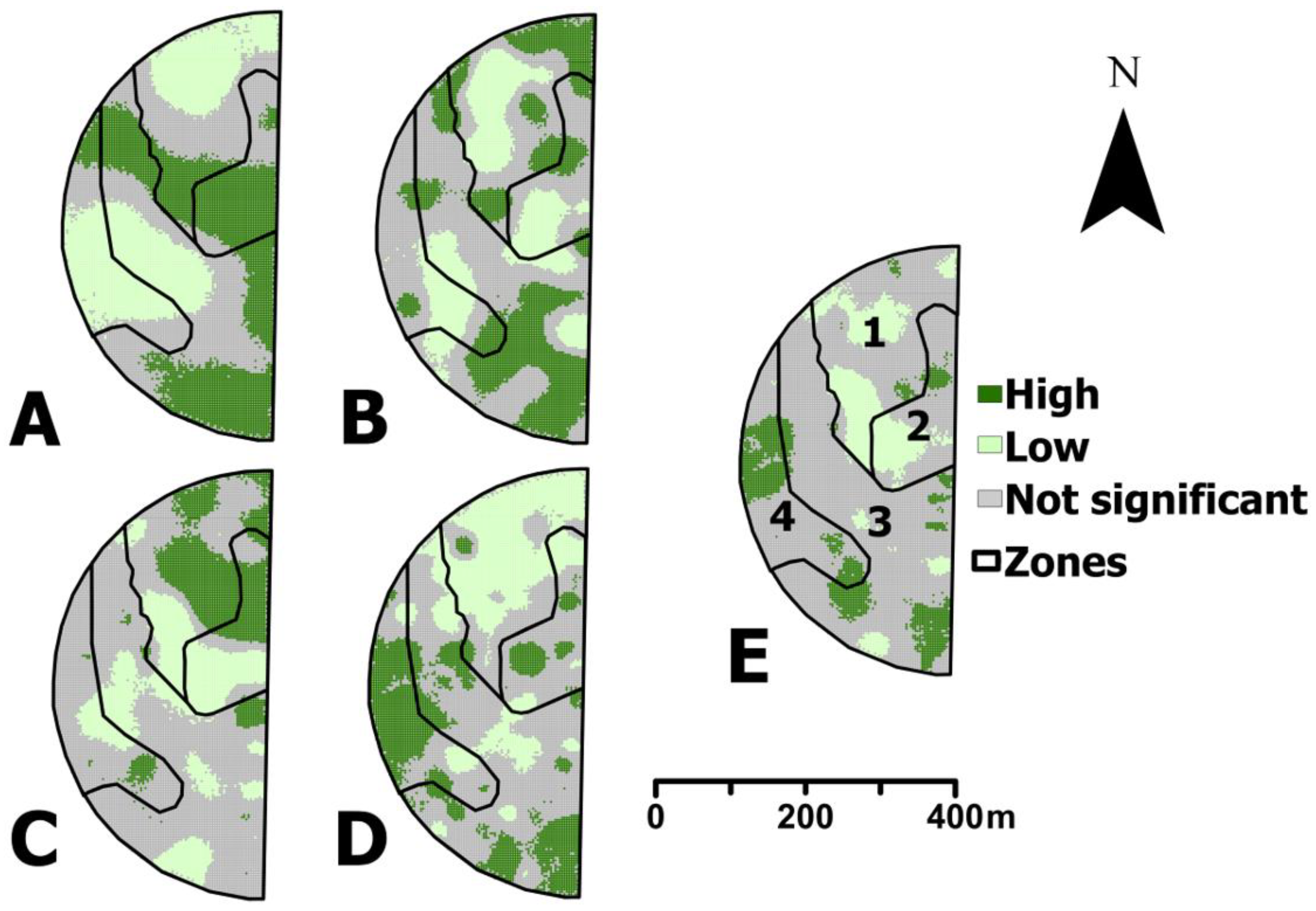
2.4. Management Zone Delineation

One approach to account for multi-variable variability in management zone delineation is to use a principle components analysis (PCA). PCA preserves the variability in the dataset while reducing dimensionality [39]. VRI management zones were delineated using principal components generated from the standardized z-scores of the alfalfa biomass yield in 2022, a United States Geological Survey (USGS) digital elevation model, and initial soil moisture samples taken on 12 May 2021 and 20 April 2022 at the 66 points in the field [40]. The principal component values were used with a K means clustering analysis to create 2 to 8 zones. Mean squared error (MSE) values were recorded for each number of zones. A scree plot was created to show how the number of zones influenced the MSEs and to determine the optimal number of zones [39].

2.5. UAV Imagery Acquisition

Imagery was obtained using the Da-Jiang Innovations (DJI) Phantom 4 (Da-Jiang Innovations, Shenzhen, China) and DJI Phantom 4 Real Time Kinematics (RTK) systems. The Phantom 4 had a Sentera RGB sensor (~17 cm resolution) and was used for the 2021 season. The camera was a 2.54 cm complementary metal oxide semiconductor (CMOS) sensor with 20 M effective pixels and was set to be parallel to the ground, nadir. The Phantom 4 RTK was used for all flights in 2022. The Phantom 4 RTK system had a 2.54 cm CMOS RGB sensor (~17 cm resolution). The UAVs were programmed to take photos with 80% frontal and 80% side overlap [11] and were geotagged using the onboard global positioning system (GPS). The UAVs were equipped with a 3-axis-gimbal to stabilize the camera during the flights. The field was mapped at 118 m above ground level (AGL) for all flights. The UAV speed was between 25 and 40 km h−1. Images were collected during the optimum UAV operating hours (11 am–2 pm) to decrease shadows. The best management practices were followed for all flights. The UAV followed the same automated flight plan created using DroneDeploy for the study (DroneDeploy, 2021).

2.6. Image Processing

The UAV imagery was processed using Web Open Drone Mapping (WebODM) and the scale-invariant feature transform (SIFT) algorithm [41]. The individual images from each flight were stitched together using common local features, creating a sparse point-cloud of tie points to create an orthomosaic [31]. The GPS geometric accuracy was reported to be 0.39 m. The orthomosaics were imported into ArcGIS Pro (ESRI, ArcGIS desktop: Release 2.24, Redlands, CA, USA). The blue wavelengths of light were from 450 to 510 nm, the green wavelengths of light were from 530 to 590 nm, and the red wavelengths of light were from 640 to 670 nm. Imagery was post-processed via geometrical correction to ensure correct easting and northing locations.

2.7. Resampling Methods

Both the DJI Phantom 4 and DJI Phantom 4 RTK UAVs had spatial resolutions of 0.17 m at 118 m AGL. A resolution this fine introduces some noise to data and can be inappropriate for the remote estimation of LAI and other vegetation indices [42]. Resolutions between 0.5 and 5 m are more accurate for LAI estimation [36]. Direct and ladder methods are the two main ways of resampling imagery to gain a coarser, more appropriate resolution. A ladder resampling method to 3 m resolution was used [11]. Resampling was conducted via ArcGIS Pro by importing the orthomosaic bands and using the ladder method listed below. The native 0.17 m resolution of each band was resampled to 0.25 m, 0.25 m to 0.50 m, 0.50 m to 1 m, 1 m to 2 m, and 2 m to 3 m [11] using the nearest neighbor resampling method [2,43].

2.8. Visible Vegetation Indices (VVIs) Calculations

There are many visible vegetation indices (VVIs), from very simple to very complex [44]. Eleven VVIs were selected because of their sensitivity to alfalfa growth and LAI [11,22,44] (Table 2). Each index differs based on the ratios of visible wavelengths (red, green, and blue). VVIs were calculated using the raster calculator tool in ArcGIS Pro on the resampled 3 m resolution imagery for each sample date. VVI values for each of the 66 sampling points were extracted using the extract multi-value to points tool in ArcGIS Pro (Supplementary Materials). VVI values were averaged for each of the management zones for each flight. The zone-average VVIs were then compared to the manually measured zone-averaged LAI values using simple linear regression models.

2.9. Model Development and Validation Datasets

All the calculated VVIs, measured alfalfa canopy heights, and the measured LAI (m2 m−2) for each of the 66 sampling points across the 9 sampling dates were compiled into 1 dataset (n = 574). A random number generator was applied to each of the data points. The data were then arranged in ascending order and the 1st 2/3 (n = 379) were put into a model development dataset. The remaining 1/3 (n = 195) of the data was reserved to validate the model development LAI equations. The zone averages across the sampling dates were used to create the average LAI, alfalfa canopy height, and VVIs. The model development data were then imported into R software (v.4.1.1, R Development Core Team, 2022) to run linear regressions of each VVI to the LAI.

2.10. Regression Modeling

Each of the VVIs (Table 2) were used as independent variables in a simple linear regression (SLR) of the model development data to predict the measured LAI m2 m−2. The field average alfalfa canopy height was used in multiple linear regression (MLR) to improve the prediction of LAI from VVIs. The four models with the highest coefficient of determination without field average height were selected and the four equations with the highest coefficient of determination with field average canopy height were selected from the model development dataset and applied to the model validation dataset to predict the LAI.

2.11. Model Evaluation Statistics

Three model statistics, relative error, root mean squared error, and normalized objective function, were calculated for each of the VVI models to evaluate performance. Relative error (RE) shows the bias of the predicted mean in relation to the measured mean. Root mean square error (RMSE) shows the error in the predictions. The normalized objective function (NOF) shows the average deviation between the predicted and observed values. The equation for the relative error is
RE = P O P 100  
where P is the predicted mean and O is the observed mean. RE is the average over the entire dataset, showing long-term bias. A negative RE value expresses the model bias toward underestimation, and a positive RE value expresses model overestimation. However, bias alone is not enough. A small RE could be the result of over- and underestimations that cancel each other out. RMSE negates this problem of under- or overestimation by averaging the squared differences, weighing larger differences more heavily. The equation for RMSE is
RMSE = i = 1 n P i O i 2 n
where Pi is the ith predicted value, Oi is the ith observed value, and n is the number of samples. The equation for NOF is
NOF = RMSE O
where RMSE and O are as previously defined. A NOF value of 0 indicates a perfect fit between the experimental and simulated results, and an NOF value less than 1 is a simulation error less than 1 standard deviation from the experimental mean.

2.12. Zone Statistical Analysis

Once the selected equations for predicting LAI were validated using the 1/3 validation dataset, 1 equation with the highest R2 value was applied to the 3 m resolution UAV images. A total of 150 random samples for each of the 4 zones were selected using the random sampling tool in ArcGIS Pro to test the zone UAV-predicted LAI against the field mean LAI [11]. The UAV-predicted LAI value at each sample point was recorded and an analysis of variance (ANOVA) test was performed for each sampling date across the zones. If the p-value was <0.05, a Bonferroni test was performed between each zone to indicate which zones were statistically different from each other.

3. Results

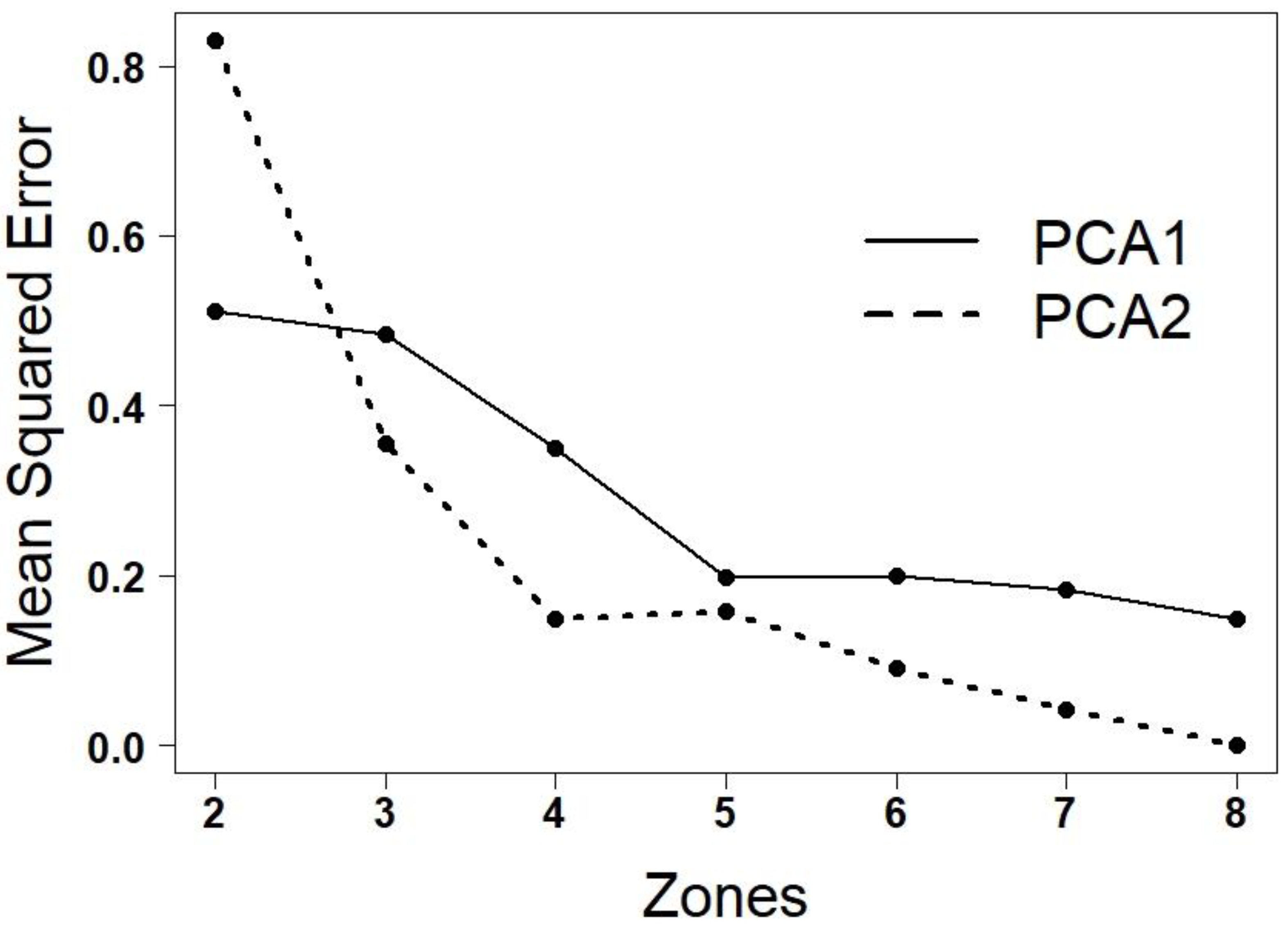
3.1. Number of Management Zones

The scree plot shows that as the number of zones increases, the mean squared error (MSE) for Principal Component 1 (PCA1) and Principal Component 2 (PCA2) decreases (Figure 2). In a scree plot, the point where there is the greatest change in slope identifies the optimal number of zones. For this study, a four-zone pattern (Figure 3) was chosen to represent the alfalfa field as PCA 1 and 2 suggested that four or five zones were optimal for this dataset (Figure 2).

3.2. Variability in Measured Alfalfa Leaf Area Index and Canopy Height

The measured LAI for alfalfa varied temporally from the beginning of the growing season, 12 May 2021 and 10 May 2022, to shortly before the harvest, 1 June 2021 and 15 June 2022 (Table 3). As the alfalfa grew, the LAI increased across the field with the greatest temporal change happening within the week of 7–15 June 2022. During this week, alfalfa produced more leaves and grew laterally, which greatly increased LAI.
For each date that LAI was measured, unique spatial patterns of LAI existed. The within-field spatial variability was evaluated using a univariate Moran’s I test of spatial autocorrelation. Each date had a positive Moran’s I value and significant p-value (Table 4), showing that there was significant positive spatial autocorrelation or the clustering of high and low values. At the beginning, throughout, and at the end of the season for both years, there were differences in where the significant clusters of the high and low LAI were located in the field (Figure 4). The greatest difference in the zone-averaged LAI values was between Zone 1 and Zone 4 at the end of the alfalfa growth period (p < 0.05) (Figure 4). An overall pattern of statistically high, low, and non-significant points was created for the nine dates that the LAI was measured on. There was no defined negative spatial autocorrelation present and no spatial outliers.
The alfalfa measured canopy height varied temporally with dates ranging from the beginning of the growing season, 12 May 2021 and 10 May 2022, to right before the harvest, 1 June 2021 and 15 June 2022 (Table 3). At the beginning of the 2021 growing season, the alfalfa canopy height varied from 16 to 25 cm with a mean of 20 cm and standard deviation of 1.96 cm, and for 2022 it varied from 6 to 18 cm with a mean of 14 cm and standard deviation of 2.19 cm (Table 3). The alfalfa canopy height increased temporally with a linear pattern of growth throughout each harvest.

3.3. Evaluation of Visible Vegetation Indices and Height

The eleven VVIs were calculated for each of the nine days that UAV data were acquired and LAI was measured. Each of the VVIs showed variation across the field and across the dates (Supplemental Data). The four VVIs with the highest coefficient of determination in the model development dataset for the SLRs were ExGR (R2 = 0.53), ExR (R2 = 0.39), the MGRVI (R2 = 0.35), and the NGRDI (R2 = 0.35) (Table 5). The four VVIs with the highest coefficient of determination in the model development dataset for the MLRs that included average canopy height were the MGRVI (R2 = 0.94), NGRDI (R2 = 0.94), ExR (R2 = 0.94), and ExGR (R2 = 0.92) indices (Table 3).
As one example of how canopy height improves the correlation of VVIs to LAI, the MGRVI equation with canopy height was applied to the validation dataset to assess the performance of the model (Figure 5). The RMSE was 0.67, the RE was 0.39, and the NOF was 0.16. The UAV prediction model had a linear relationship with the measured LAI which was significant (p < 0.05).
Throughout the growing season, the UAV-predicted LAI was consistent with the measured LAI. The trendline was close to the 1:1 line and was highly correlated with the measured LAI. While the UAV-predicted LAI model slightly overestimated LAI at values above 4, using the field average height overcame the point of saturation problem observed when UAV imagery was used alone to predict LAI.

3.4. Zone Statistical Analysis

The model developed using the MLR of the MGRVI and average canopy height was applied to each of the 3 m resolution UAV orthomosaic images to predict LAI where it was not manually measured. There were not distinct, repeating visual patterns between the zones when the equation was applied (Figure 6). The images from the beginning of the growing season in 2021 (Figure 6A) and 2022 (Figure 6D) show areas of the field with very low LAI values. These were noticeable in the field as spots with delayed alfalfa growth and were green in areas where snow and ice persisted the longest. These patterns disappeared over time. More pronounced spatial variation in the predicted LAI was observed on 29 June 2021 (Figure 6B, sixteen days before second harvest) and 2 June 2022 (Figure 6E, thirteen days before first harvest). The least spatial variation in LAI was observed for times with maximum growth as alfalfa approached the time for harvest on 1 June 2021 (Figure 6C, seven days before first harvest) and 15 June 2022 (Figure 6F, one day before first harvest).
The average predicted LAI value per zone was calculated from 150 random sample points in each zone and compared to the field-average-predicted LAI to determine whether there was enough within-field spatial variation to warrant VRI in this alfalfa field (Table 6). At the beginning of the growing season, the greatest LAI zone differences were observed. As the alfalfa grew, the differences between the zones decreased. There were no two zones that reached a 15% threshold difference between them [11]. This suggests that variation in the LAI values alone in this irrigated alfalfa field was not enough to direct full-season VRI.

4. Discussion

4.1. Spatiotemporal Variability in Measured LAI

The measured LAI values varied spatially and temporally as the alfalfa grew throughout each season. For all of the dates, there were areas of the field with statistically higher and lower LAI values; however, the observed spatial patterns were not consistent over time. In a study on predicting LAI of grassland from VVIs, Li [25] also showed that the spatial patterns of the predicted LAI varied over time. In the Li [25] study, the spatial patterns for LAI changed in response to the growth of different plant species. Changes in the growth of different species do not explain the observation in this study of an alfalfa monoculture. Rather, the spatiotemporal variation observed in this study was mostly controlled by the alfalfa development stage.
While it was not an objective of this study to explain the causation of spatial variation in the LAI, we observed several influencing factors. For example, in both 2021 and 2022, the late melting of snow and ice resulted in areas of the field with a relatively low LAI during the first LAI measurements of the year (Figure 6A,D). We also speculate that spatial patterns in LAI are related to plant available water and how this may vary throughout the root zone. The surface soils at this study site were much drier in 2022 than in 2021 and this likely influenced the observed differences in the LAI between the years. It is interesting to note that in the 29 June 2021 UAV imagery (Figure 4B), a semi-circular pattern was visible that corresponded to a temporary problem with water delivery in that part of the center-pivot irrigation system. This observation supports the hypothesis that water availability may explain other observed spatial patterns in the LAI. Other studies such as that by Kayad et al. [17] have shown that spatial variation in alfalfa biomass was explained by slope, flow accumulation, and the topographic wetness index. These factors are interesting because of the potential for temporal variation, as they interact with dynamic factors including precipitation and solar radiation.

4.2. Visible Vegetation Index for Alfalfa Leaf Area Index Estimation

The MGRVI, NGRDI, and ExR were the models with the highest coefficient of determination compared to the other VVIs in the study, especially when alfalfa height was included. All VVIs’ coefficient of determination values increased when height was incorporated into the MLR models. The models that performed the poorest were those in which the blue wavelengths of light were more heavily weighted. This suggests similar results to Hopkins [11] in that the blue wavelength is less useful for LAI estimation in wheat.
Though Hopkins [11] and Li [22] both had VARI and NGRDI as their models with the highest coefficient of determinations for wheat and rice, respectively [11,22], VARI was ranked number 6 out of 11 indices for alfalfa with a R2 value of 0.22 in the SLR. With the addition of average field height, the VARI’s coefficient of determination increased to a R2 of 0.90. Alfalfa has a multiple-layered leaf structure that makes correlating VVIs with the LAI more difficult [54]. This additional complexity means that when the alfalfa canopy becomes saturated, there will not be proportionally the same change in light reflected back off the plant, which would increase the LAI values [55]. However, when the field average alfalfa canopy height is known, it can be used to supplement the VVIs and greatly increase the correlation with LAI.
One approach to estimating alfalfa canopy height remotely is using photogrammetric techniques such as the structure from motion algorithm [29]. Structure from motion is the analysis of feature matching common points in multiple images and creating a three-dimensional point cloud that can be used to create a digital terrain model (DTM) and digital surface model (DSM) of the field. In this study, we manually measured the alfalfa canopy height, which may not be practical for wide applications. Using the same UAV imagery, there is the potential to estimate the plant height by subtracting the DTM from the DSM [56]. However, the accuracy of the DTM can be inhibited under dense canopies such as alfalfa [57].

4.3. Translation of UAV Images of the Entire Field

At the beginning of the season, there were areas of the field where alfalfa had not started to grow and were easily detected from the LAI prediction model (Figure 6A,D). The greatest spatial difference among zone-estimated LAI existed early within the first harvest interval (Table 5). As the alfalfa matures, the differences in average estimated LAI decrease among the pre-determined zones [55]. Though some zones are statistically different from each other, no two zones reach a 15% threshold difference in the LAI values needed [11]. This threshold of 15% difference was based on the practical ability of the center-pivot sprinkler to be able to apply different rates among VRI zones. The observed spatial patterns (Figure 6) may approach practical differences if dynamic zones are delineated for each UAV flight date rather than the static zones used in this analysis.

4.4. Limitations and Future Work

A key aspect of this study was the determination of VRI zones based on a PCA using alfalfa biomass yield, relative elevation, and pre-season soil water content. The spatial variation in the LAI did not align well with these zones. Thus, future work could address alternative approaches for zone delineation. One potential approach is the use of independent component analysis (ICA), an approach that shows spatial heterogeneity and reduces dimensionality in data. The ICA approach has been demonstrated to be a zone delineation mechanism in soybean, spring wheat, and winter wheat [58]. Other future work could also expand upon the variables used for zone delineation for either PCA or ICA methods. One variable shown to possess importance in other studies is the soil apparent electrical conductivity [59,60]. Future work could also explore the potential for using temporally dynamic zones rather than static zones.
Measuring the alfalfa canopy height proved to be important in estimating LAI. All VVI models were improved when the field average canopy height was included in the MLR. Manually measuring the canopy height across the field can be time-intensive. A potentially more efficient way to estimate canopy height is remotely, with structure for motion techniques from UAV imagery. Howell [56] examined different UAV flight parameters to estimate Mountain big sagebrush (Artemisia tridentata spp. vaseyana) canopy height via UAV imagery. The authors found that they could estimate sagebrush canopy height within 10 cm (standard error: 0.4 cm) of the actual height using UAV imagery. Xie [29] found that you can estimate the canopy height of rapeseed using UAV imagery with structure for motion techniques (RMSE: 3 cm). These techniques for estimating canopy height via UAV imagery need to be studied for alfalfa.

4.5. Conclusions

The results showed that UAV imagery that acquired the MGRVI, NGRDI, and ExR vegetation indices along with measured field average canopy height could predict LAI across the growing season (R2 = 0.94, R2 = 0.94, R2 = 0.94, and R2 = 0.92). The most useful VVIs identified for alfalfa in this study were different to those that Hopkins [11] and Li [22] reported for wheat and rice, respectively. VVIs with canopy height showed promising results for using UAV imagery to predict LAI in alfalfa. VVI- and canopy-height-derived models can be used to estimate LAI and zone-specific Kc; however, the difference in the LAI between zones for this alfalfa field was not above a 15% threshold, which was assumed to be the practical level needed to justify the use of VRI. If different and temporally dynamic management zones are used, the LAI approach presented may have practical use in VRI applications. VVIs alone are appropriate to use to estimate the LAI for rice and wheat, but alfalfa is more structurally complicated and an average height for the field is needed to improve the model of the LAI from VVIs.

Supplementary Materials

The following supporting information can be downloaded at https://www.mdpi.com/article/10.3390/agronomy13051289/s1.

Author Contributions

Conceptualization, R.R.J., M.A.Y., A.P.H. and N.C.H.; methodology, K.H., R.K., R.R.J. and A.P.H.; software, K.H., R.K. and R.R.J.; validation, K.H., R.K., A.P.H. and N.C.H.; formal analysis, K.H. and R.K.; investigation, N.C.H.; resources, R.R.J., R.S. and N.C.H.; data curation, K.H.; writing—original draft preparation, K.H., A.P.H. and N.C.H.; writing—review and editing, K.H., R.K., R.R.J., R.S., A.H., B.G.H., M.A.Y., A.P.H. and N.C.H.; visualization, K.H. and R.K.; supervision, N.C.H.; project administration, N.C.H.; funding acquisition, B.G.H., M.A.Y. and N.C.H. All authors have read and agreed to the published version of the manuscript.

Funding

This research was funded by US-Israel Agricultural Research and Development Fund, IS-5218-19, and USDA Western Sustainable Agriculture Research and Education Program, SW19-909. The APC was funded by Brigham Young University.

Data Availability Statement

Interested parties can contact the corresponding author regarding data availability.

Acknowledgments

Several people not listed as authors assisted with the field surveys that this paper is based on: Alvin Lusk, Kaitlin Bair, Thomas Armstrong, Kayla Marion, Alton Campbell, Samantha Shumate, Caden Seely, Alexandra Olsen, Miria Barnes, Braxton Underwood, and William Burnett.

Conflicts of Interest

The authors declare no conflict of interest.

References

  1. Zhao, W.; Li, J.; Yang, R.; Li, Y. Crop Yield and Water Productivity Responses in Management Zones for Variable-Rate Irrigation Based on Available Soil Water Holding Capacity. Trans. ASABE 2017, 60, 1659–1667. [Google Scholar] [CrossRef]
  2. Chandel, A.K.; Molaei, B.; Khot, L.R.; Peters, R.T.; Stöckle, C.O. High Resolution Geospatial Evapotranspiration Mapping of Irrigated Field Crops Using Multispectral and Thermal Infrared Imagery with METRIC Energy Balance Model. Drones 2020, 4, 52. [Google Scholar] [CrossRef]
  3. O’Shaughnessy, S.A.; Evett, S.R.; Andrade, A.; Workneh, F.; Price, J.A.; Rush, C.M. Site-Specific Variable Rate Irrigation as a Means to Enhance Water Use Efficiency. In Proceedings of the Irrigation Symposium: Emerging Technologies for Sustainable Irrigation, Long Beach, CA, USA, 10–12 November 2015. [Google Scholar]
  4. Svedin, J.D.; Kerry, R.; Hansen, N.C.; Hopkins, B.G. Identifying Within-Field Spatial and Temporal Crop Water Stress to Conserve Irrigation Resources with Variable-Rate Irrigation. Agronomy 2021, 11, 1377. [Google Scholar] [CrossRef]
  5. Hu, Y.; Kang, S.; Ding, R.; Du, T.; Tong, L.; Li, S. The Dynamic Yield Response Factor of Alfalfa Improves the Accuracy of Dual Crop Coefficient Approach under Water and Salt Stress. Water 2020, 12, 1224. [Google Scholar] [CrossRef]
  6. Chen, W.; Shen, Y.; Robertson, M.; Probert, M.; Bellotti, B.; Nan, Z. Simulation of crop growth and soil water for different cropping systems in the Gansu Loess Plateau, China using APSIM. In Proceedings of the 4th International Crop Science Congress, Brisbane, Australia, 26 September–1 October 2004. [Google Scholar]
  7. Yang, X.; Brown, H.E.; Texixeira, E.I.; Moot, D.J. Development of a lucerne model in APSIM next generation: 2 canopy expansion and light interception of genotypes with different fall dormancy ratings. Eur. J. Agron. 2022, 139, 126570. [Google Scholar] [CrossRef]
  8. Dejonge, K.C.; Thorp, K.R. Implementing Standardized Reference Evapotranspiration and Dual Crop Coefficient Approach in the DSSAT Cropping System Model. Trans. ASABE 2017, 60, 1965–1981. [Google Scholar] [CrossRef]
  9. Irmak, S.; Odhiambo, L.O.; Specht, J.E.; Djaman, K. Hourly and Daily Single and Basal Evapotranspiration Crop Coefficients as a Function of Growing Degree Days, Days After Emergence, Leaf Area Index, Fractional Green Canopy Cover, and Plant Phenology for Soybean. Trans. ASABE 2013, 56, 1785–1803. [Google Scholar] [CrossRef]
  10. Al-Kaisi, M.; Brun, L.J.; Enz, J.W. Transpiration and evapotranspiration from maize as related to leaf area index. Agric. For. Meteorol. 1989, 48, 111–116. [Google Scholar] [CrossRef]
  11. Hopkins, A.P. Remote Sensing and Spatial Variability of Leaf Area Index of Irrigated Wheat Fields. Master’s Thesis, Brigham Young University, Provo, UT, USA, 2021. [Google Scholar]
  12. Kompanizare, M.; Petrone, R.M.; Macrae, M.L.; De Haan, K.; Khomik, M. Assessment of effective LAI and water use efficiency using Eddy Covariance data. Sci. Total Environ. 2022, 802, 149628. [Google Scholar] [CrossRef]
  13. Walter-Shea, E. Relations between directional spectral vegetation indices and leaf area and absorbed radiation in Alfalfa. Remote Sens. Environ. 1997, 61, 162–177. [Google Scholar] [CrossRef]
  14. Sharratt, B.S.; Baker, D.G. Alfalfa Leaf Area as a Function of Dry Matter1. Crop Sci. 1986, 26, 1040–1043. [Google Scholar] [CrossRef]
  15. Al-Gaadi, K.A.; Patil, V.C.; Tola, E.H.M.; Madugundu, R.; Marey, S.A.; Al-Omran, A.M.; Al-Dosari, A. Variable Rate Application Technology for Optimizing Alfalfa Production in Arid Climate. Int. J. Agric. Biol. 2015, 17, 71–79. [Google Scholar]
  16. Chandel, A.K.; Yu, L.-X. Alfalfa (Medicago sativa L.) crop vigor and yield characterization using high-resolution aerial multispectral and thermal infrared imaging technique. Comput. Electron. Agric. 2021, 182, 105999. [Google Scholar] [CrossRef]
  17. Kayad, A.G.; Al-Gaadi, K.A.; Tola, E.; Madugundu, R.; Zeyada, A.M.; Kalaitzidis, C. Assessing the Spatial Variability of Alfalfa Yield Using Satellite Imagery and Ground-Based Data. PLoS ONE 2016, 11, e0157166. [Google Scholar] [CrossRef] [PubMed]
  18. Feng, L.; Zhang, Z.; Ma, Y.; Du, Q.; Williams, P.; Drewry, J.; Luck, B. Alfalfa Yield Prediction Using UAV-Based Hyperspectral Imagery and Ensemble Learning. Remote Sens. 2020, 12, 2028. [Google Scholar] [CrossRef]
  19. Hu, Q.; Yang, J.; Xu, B.; Huang, J.; Memon, M.S.; Yin, G.; Zeng, Y.; Zhao, J.; Liu, K. Evaluation of Global Decametric-Resolution LAI, FAPAR and FVC Estimates Derived from Sentinel-2 Imagery. Remote Sens. 2020, 12, 912. [Google Scholar] [CrossRef]
  20. Veroustraete, F. The Rise of the Drones in Agriculture. EC Agric. 2015, 2, 325–327. [Google Scholar]
  21. Viña, A.; Gitelson, A.A.; Nguy-Robertson, A.L.; Peng, Y. Comparison of different vegetation indices for the remote assessment of green leaf area index of crops. Remote Sens. Environ. 2011, 115, 3468–3478. [Google Scholar] [CrossRef]
  22. Li, S.; Yuan, F.; Ata-Ui-Karim, S.T.; Zheng, H.; Cheng, T.; Liu, X.; Tian, Y.; Zhu, Y.; Cao, W.; Cao, Q. Combining Color Indices and Textures of UAV-Based Digital Imagery for Rice LAI Estimation. Remote Sens. 2019, 11, 1763. [Google Scholar] [CrossRef]
  23. Broge, N.H.; Leblanc, E. Comparing prediction power and stability of broadband and hyperspectral vegetation indices for estimation of green leaf area index and canopy chlorophyll density. Remote Sens. Environ. 2000, 76, 156–172. [Google Scholar] [CrossRef]
  24. Xue, J.; Su, B. Significant Remote Sensing Vegetation Indices: A Review of Developments and Applications. J. Sens. 2017, 2017, 1353691. [Google Scholar] [CrossRef]
  25. Li, Z. Improved Leaf Area Index Estimation by Considering Both Temporal and Spatial Variations. Master’s Thesis, University of Saskatchewan, Saskatoon, SK, Canada, 2010. [Google Scholar]
  26. Li, Y.; Su, D. Alfalfa Water Use and Yield under Different Sprinkler Irrigation Regimes in North Arid Regions of China. Sustainability 2017, 9, 1380. [Google Scholar] [CrossRef]
  27. Grimes, D.W.; Wiley, P.L.; Sheesley, W. Alfalfa yield and plant water relations with variable irrigation. Crop Sci. 1992, 32, 1381–1387. [Google Scholar] [CrossRef]
  28. Wang, L.; Xie, J.; Luo, Z.; Niu, Y.; Coulter, J.A.; Zhang, R.; Lingling, L. Forage yield, water use efficiency, and soil fertility response to alfalfa growing age in the semiarid Loess Plateau of China. Agric. Water Manag. 2021, 243, 106415. [Google Scholar] [CrossRef]
  29. Xie, T.; Li, J.; Yang, C.; Jiang, Z.; Chen, Y.; Guo, L.; Zhang, J. Crop height estimation based on UAV images: Methods, errors, and strategies. Comput. Electron. Agric. 2021, 185, 106155. [Google Scholar] [CrossRef]
  30. Staff, S.S. Web Soil Survey. Available online: http://websoilsurvey.sc.egov.usda.gov/ (accessed on 6 January 2021).
  31. Kaivosoja, J.; Hautsalo, J.; Heikkinen, J.; Hiltunen, L.; Ruuttunen, P.; Näsi, R.; Niemeläinen, O.; Lemsalu, M.; Honkavaara, E.; Salonen, J. Reference Measurements in Developing UAV Systems for Detecting Pests, Weeds, and Diseases. Remote Sens. 2021, 13, 1238. [Google Scholar] [CrossRef]
  32. Pittman, J.; Arnall, D.; Interrante, S.; Moffet, C.; Butler, T. Estimation of Biomass and Canopy Height in Bermudagrass, Alfalfa, and Wheat Using Ultrasonic, Laser, and Spectral Sensors. Sensors 2015, 15, 2920–2943. [Google Scholar] [CrossRef]
  33. Chang, K.-T.; Hsu, W.-L. Estimating Soil Moisture Content Using Unmanned Aerial Vehicles Equipped with Thermal Infrared Sensors. In Proceedings of the IEEE Internation Conference on Applied System Innovation, Chiba, Japan, 13–17 April 2018; pp. 168–171. [Google Scholar]
  34. Ten Harkel, J.; Bartholomeus, H.; Kooistra, L. Biomass and Crop Height Estimation of Different Crops Using UAV-Based Lidar. Remote Sens. 2019, 12, 17. [Google Scholar] [CrossRef]
  35. Decagon Devices, Inc. AccuPAR PAR/LAI Ceptometer Model LP-80 Operator’s Manual; METER Group: Pullman, WA, USA, 2013; p. 82. [Google Scholar]
  36. Atkinson, P.M. Selecting the spatial resolution of airborne MSS imagery for small-scale agricultural mapping. Int. J. Remote Sens. 1997, 18, 1903–1917. [Google Scholar] [CrossRef]
  37. Kerry, R.; Oliver, M.A. Variograms of Ancillary Data to Aid Sampling for Soil Surveys. Precis. Agric. 2003, 4, 261–278. [Google Scholar] [CrossRef]
  38. Walthall, C.L.; Pachepsky, Y.; Dulaney, W.P.; Timlin, D.J.; Daughtry, C.S.T. Exploitation of spatial information in high resolution digital imagery to map leaf area index. Precis. Agric. 2007, 8, 311–321. [Google Scholar] [CrossRef]
  39. Woolley, E. Soil Water Dynamics within Variable Rate Irrigation Zones of Winter Wheat. Master’s Thesis, Brigham Young University, Provo, UT, USA, 2021. [Google Scholar]
  40. Haghverdi, A.; Leib, B.G.; Washington-Allen, R.A.; Ayers, P.D.; Buschermohle, M.J. Perspectives on delineating management zones for variable rate irrigation. Comput. Electron. Agric. 2015, 117, 154–167. [Google Scholar] [CrossRef]
  41. Hu, Q.; Mingyao, A. Scale Invariant Feature Transform based matching approach to Unmanned Aerial Vehicles image geo-reference with large rotation angle. In Proceedings of the IEEE International Conference on Spatial Data Mining and Geographical Knowledge Services (ICSDM), Fuzhou, China, 29 June–1 July 2011. [Google Scholar]
  42. Curran, P.J.; Dawn Williamson, H. Selecting a spatial resolution for estimation of per-field green leaf area index. Int. J. Remote Sens. 1988, 9, 1243–1250. [Google Scholar] [CrossRef]
  43. Gurjar, S.B.; Padmanabhan, N. Study of various resampling techniques for high-resolution remote sensing imagery. J. Indian Soc. Remote Sens. 2005, 33, 113–120. [Google Scholar] [CrossRef]
  44. Payero, J.O.; Neale, C.M.U.; Wright, J.L. Comparison of eleven vegetation indices for estimating plant height of alfalfa and grass. Appl. Eng. Agric. 2004, 20, 385–393. [Google Scholar] [CrossRef]
  45. Mao, W.; Wang, Y.; Wang, Y. Real-Time Detection of Between-Row Weeds Using Machine Vision; American Society of Agricultural and Biological Engineers: St. Joseph, MI, USA, 2003. [Google Scholar]
  46. Woebbecke, D.M.; Meyer, G.E.; Von Bargen, K.; Mortensen, D.A. Color Indices for Weed Identification Under Various Soil, Residue, and Lighting Conditions. Trans. ASAE 1995, 38, 259–269. [Google Scholar] [CrossRef]
  47. Meyer, G.E.; Neto, J.C. Verification of color vegetation indices for automated crop imaging applications. Comput. Electron. Agric. 2008, 63, 282–293. [Google Scholar] [CrossRef]
  48. Camargo Neto, J. A Combined Statistical-Soft Computing Approach for Classification and Mapping Weed Species in Minimum -Tillage Systems. Ph.D. Thesis, The University of Nebraska-Lincoln, Ann Arbor, MI, USA, 2004. [Google Scholar]
  49. Louhaichi, M.; Borman, M.M.; Johnson, D.E. Spatially Located Platform and Aerial Photography for Documentation of Grazing Impacts on Wheat. Geocarto Int. 2001, 16, 65–70. [Google Scholar] [CrossRef]
  50. Kawashima, S.; Nakatani, M. An Algorithm for Estimating Chlorophyll Content in Leaves Using a Video Camera. Ann. Bot. 1998, 81, 49–54. [Google Scholar] [CrossRef]
  51. Tucker, C.J. Red and photographic infrared linear combinations for monitoring vegetation. Remote Sens. Environ. 1979, 8, 127–150. [Google Scholar] [CrossRef]
  52. Bendig, J.; Yu, K.; Aasen, H.; Bolten, A.; Bennertz, S.; Broscheit, J.; Gnyp, M.L.; Bareth, G. Combining UAV-based plant height from crop surface models, visible, and near infrared vegetation indices for biomass monitoring in barley. Int. J. Appl. Earth Obs. Geoinf. 2015, 39, 79–87. [Google Scholar] [CrossRef]
  53. Gitelson, A.A.; Gritz, Y.; Merzlyak, M.N. Relationships between leaf chlorophyll content and spectral reflectance and algorithms for non-destructive chlorophyll assessment in higher plant leaves. J. Plant Physiol. 2003, 160, 271–282. [Google Scholar] [CrossRef] [PubMed]
  54. Alam, A.; Yamamoto, S.; Kahn, N.; Honna, T. Screening for agronomic performance of six indigenous cultivars of alfalfa (Medicago sativa) at Karina northern areas of Pakistan. Electron. J. Environ. Agric. Food Chem. 2009, 8, 950–968. [Google Scholar]
  55. Xie, Q.; Dash, J.; Huang, W.; Peng, D.; Qin, Q.; Mortimer, H.; Casa, R.; Pignatti, S.; Laneve, G.; Pascucci, S.; et al. Vegetation Indices Combining the Red and Red-Edge Spectral Information for Leaf Area Index Retrieval. IEEE J. Sel. Top. Appl. Earth Obs. Remote Sens. 2018, 11, 1482–1493. [Google Scholar] [CrossRef]
  56. Howell, R.G.; Jensen, R.R.; Petersen, S.L.; Larsen, R.T. Measuring Height Characteristics of Sagebrush (Artemisia sp.) Using Imagery Derived from Small Unmanned Aerial Systems (sUAS). Drones 2020, 4, 6. [Google Scholar] [CrossRef]
  57. Wallace, L.; Lucieer, A.; Malenovský, Z.; Turner, D.; Vopěnka, P. Assessment of Forest Structure Using Two UAV Techniques: A Comparison of Airborne Laser Scanning and Structure from Motion (SfM) Point Clouds. Forests 2016, 7, 62. [Google Scholar] [CrossRef]
  58. Mirvakhabova, L.; Pukalchik, M.; Matveev, S.; Pregubova, P.; Oseledets, I. Field heterogeneity detection based on the modified FastICA RGB-image processing. J. Phys. Conf. Ser. 2018, 1117, 012009. [Google Scholar] [CrossRef]
  59. Svedin, J.D. Characterizing the Spatial Variation of Crop Water Productivity for Variable-Rate Irrigation Management. Master’s Thesis, Brigham Young University, Provo, UT, USA, 2018. [Google Scholar]
  60. Hedley, C.B.; Yule, I.J.; Tuohy, M.P.; Vogeler, I. Key performance indicators for simulated variable-rate irrigation of variable soils in humid regions. Trans. ASABE 2009, 52, 1575–1584. [Google Scholar] [CrossRef]
Figure 1. Rexburg, Idaho (red five-pointed star) alfalfa (Medicago sativa L.) field showing the 66 sampling points (black dots). Soil samples, alfalfa canopy height, and leaf area index were recorded at each sample point.
Agronomy 13 01289 g001
Figure 2. Scree plot showing mean squared errors associated with different number of zones based on K-means classification of Principal Components 1 (PCA1) and 2 (PCA2). Each black dot represents the associated mean squared error for the number of zones. The lines (solid PCA1, dashed PCA2) represent the change in mean squared error between zones.
Agronomy 13 01289 g002
Figure 3. Rexburg, Idaho, alfalfa field delineated into four management zones formed via K-means analysis of Principal Components 1 and 2.
Agronomy 13 01289 g003
Figure 4. Statistically significant cluster of high and low measured LAI (m2 m−2) for Rexburg, Idaho, alfalfa field in 2021 and 2022. (A) 12 May 2021, (B) 2 June 2021, (C) 10 May 2022, (D) 15 June 2022, and (E) overall trend for 2021 and 2022. The zone map is outlined in each and labeled in (E) for all the figures.
Agronomy 13 01289 g004
Figure 5. The equation 5.70 × MGRVI + 0.13 × avgh − 1.80 from the model development dataset was applied to the validation dataset. The trendline is a representation of the model equation (dashed line) and a 1:1 line is represented as the solid line.
Agronomy 13 01289 g005
Figure 6. Maps of the standard deviation of LAI predicted from UAV imagery in Rexburg, Idaho, alfalfa field. (A) 12 May 2021, (B) 29 June 2021, (C) 1 June 2021 (zone numbers shown), (D) 10 May 2022, (E) 2 June 2022, and (F) 15 June 2022. The four zones are outlined in each map. LAI was predicted from the MLR equation using the MGRVI and field average height.
Agronomy 13 01289 g006
Table 1. Dates of the leaf area index (LAI), unmanned aerial vehicle (UAV) flights, and alfalfa canopy height were measured in 2021 and 2022.
Date of UAV Flight, the LAI, and Height MeasurementsHarvest IntervalDays Prior to Harvest
12 May 2021127
1 June 202117
29 June 2021216
10 May 2022137
17 May 2022130
27 May 2022120
2 June 2022113
7 June 202218
15 June 202211
Table 2. Abbreviations, names, and formulas of the eleven visible vegetative indices (VVIs) that were evaluated. Formulas were calculated using reflected light in red (R), green (G), and blue (B) wavelengths.
VVINameFormulaCitation
ExBExcess Blue Vegetation IndexExB = 1.4 B − G[45]
ExGExcess Green Vegetation IndexExG = 2 G − R − B[46]
ExRExcess Red Vegetation IndexExR = 1.4 R − G[47]
ExGRExcess Green Minus Excess Red Vegetation IndexExGR = ExG − ExR[48]
GLIGreen Leaf IndexGLI = (2 G − R − B)/(2 G + R + B)[49]
IKAWKawashima IndexIKAW = (R − B)/(R + B)[50]
MGRVIModified Green–Red Vegetation IndexMGRVI = (G2 − R2)/(G2 + R2)[51]
NGRDINormalized Green–Red Difference IndexNGRDI = (G − R)/(G + R)[51]
RGBVIRed–Green–Blue Vegetation IndexRGBVI = (G2 − B × R)/(G2 + B × R)[52]
VARIVisible Atmospherically Resistant IndexVARI = (G − R)/(G + R + B)[53]
WIWoebbecke IndexWI = (G − B)/(R − G)[46]
Table 3. Summary statistics for the measured alfalfa leaf area index (LAI) and measured alfalfa canopy height from the study site in Rexburg, Idaho (n = 66). Min: minimum, Max: maximum, Std. Dev.: standard deviation.
DateLeaf Area Index (m2 m−2)Alfalfa Canopy Height (cm)
MinMaxMeanStd. Dev.MinMaxMeanStd. Dev.
12 May 20210.233.421.930.511625201.96
1 June 20214.427.866.60.693460514.06
29 June 20211.884.843.210.622650375.29
10 May 20220.362.111.20.32618142.19
17 May 20220.674.292.630.771126202.85
27 May 20222.576.074.120.72039324.09
2 June 20223.397.075.010.812748395.14
7 June 20223.088.565.541.273658485.82
15 June 20224.711.287.661.564665574.28
Table 4. Moran’s I statistics values for measured alfalfa LAI values from the study site in Rexburg, Idaho.
12/5/211/6/2129/6/2110/5/2217/5/2227/5/222/6/227/6/2215/6/22
Moran’s value0.9940.9750.9980.9800.9730.9880.9780.9930.957
p-value<0.001<0.001<0.001<0.001<0.001<0.001<0.001<0.001<0.001
Table 5. Results of simple linear regression to predict the LAI from four visible vegetation indices (VVI), and multiple linear regression results for predicting the LAI from the VVI and average canopy height (avgh). R2: coefficient of determination, RMSE: root mean square error, RE: relative error, NOF: normalized objective function.
VVIModel DevelopmentModel Validation
Model EquationR2RMSERENOF
Models excluding average canopy height
ExGRLAI = 0.08 × ExGR − 3.910.531.511.560.36
ExRLAI = −0.11 × ExR + 5.200.391.630.520.39
MGRVILAI = 16.57 × MGRVI − 0.210.351.68−0.360.40
NGRDILAI = 31.36 × NGRDI − 0.080.351.68−0.450.40
Models including average canopy height
MGRVILAI = 5.70 × MGRVI + 0.13 × avgh − 1.800.940.670.390.16
NGRDILAI = 10.77 × NGRDI + 0.13 × avgh − 1.760.940.670.190.16
ExRLAI = −0.04 × ExR + 0.13 × avgh + 0.080.940.690.690.16
ExGRLAI = 0.02 × ExGR + 0.13 × avgh − 1.800.921.0113.080.24
Table 6. Estimated alfalfa leaf area index (LAI) values for Rexburg, Idaho, averaged by date and management zone and the percent difference between management zone and field mean. Letters after the zone mean represent zones with significantly different averages (p < 0.05): a is zone 1, b is zone 2, c is zone 3, and d is zone 4.
Management ZoneField Mean
1234
12 May 2021
Estimated LAI m2 m−21.49 bd1.66 ac1.49 bd1.65 ac1.57
% difference from mean−56−55-
1 June 2021
Estimated LAI m2 m−26.22 d6.28 d6.18 d6.07 abc6.19
% difference from mean010−2-
29 June 2021
Estimated LAI m2 m−23.96 bcd3.79 acd4.06 ab4.14 ab3.99
% difference from mean−1−524-
10 May 2022
Estimated LAI m2 m−21.19 d1.291.21 d1.35 ac1.26
% difference from mean−63−47-
17 May 2022
Estimated LAI m2 m−22.30 cd2.39 d2.45 a2.52 ab2.42
% difference from mean−5−114-
27 May 2022
Estimated LAI m2 m−24.29 d4.374.33 d4.42 ac4.36
% difference from mean−20−11-
2 June 2022
Estimated LAI m2 m−27.13 bcd6.92 ad6.91 ad7.22 abc7.05
% difference from mean1−2−22-
7 June 2022
Estimated LAI m2 m−26.43 bcd6.29 a6.22 a6.26 a6.30
% difference from mean20−1−1-
15 June 2022
Estimated LAI m2 m−27.48 d7.45 d7.47 d7.54 abc7.48
% difference from mean0001-
Disclaimer/Publisher’s Note: The statements, opinions and data contained in all publications are solely those of the individual author(s) and contributor(s) and not of MDPI and/or the editor(s). MDPI and/or the editor(s) disclaim responsibility for any injury to people or property resulting from any ideas, methods, instructions or products referred to in the content.

