3.2.1. Linear Error Discretization of the Kinematic Lawn Mower Model
According to the state equation shown in Equation (1), the system can be regarded as an input with
, and the state variables are
=
. The general form of the linear control system of
T is shown in Equation (2) [
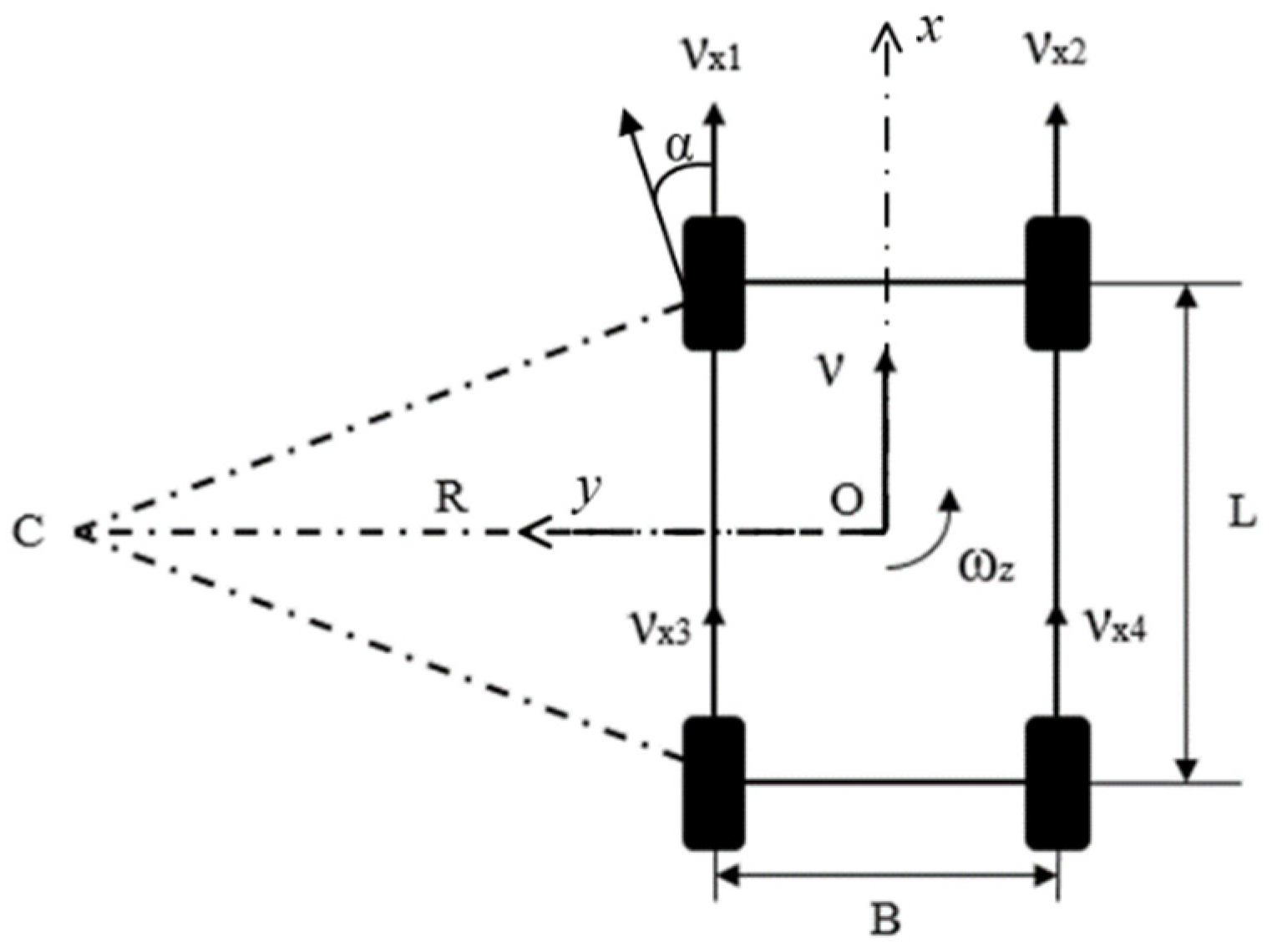
14]. The heading angle of the lawn mower,
θ, is equal to the angle between the geometric center of the lawn mower and the
x-axis.
If the working path of the mower acquired based on GPS is taken as the reference path and each path point on the reference path satisfies the established kinematic equation, then a kinematic model that satisfies the preset conditions is shown in Equation (3):
where
.
By expanding the above equation using Taylor’s formula at the first reference point of the reference path [
20] and ignoring higher-order terms, the linear error model of the lawn mower is obtained, as shown in Equation (4):
The linearized error model of the lawn mower can be calculated by combining the above two equations:
In the equation, A and B are the Jacobian matrices of f with respect to x and u, respectively; A = , and B = .
To apply the linearization error model to the MPC controller, discretization processing is performed by the forward Euler method [
22] to obtain the linear error discretization model of the system, as shown in the following equation:
where
,
,
, and
T is the sampling time.
3.2.2. Design of the Objective Function and Constraint Conditions
To prevent the control variables in the system from experiencing sudden changes, which may lead to decreases in the path-tracking accuracy and system stability of the lawn mower, control increments are used to replace the control variables. The modified state equation is as follows:
Therefore, the output state quantity of the system can be expressed as follows:
where
represents the output of the discrete MPC system,
x represents the horizontal axis position of the lawn mower,
y represents the vertical axis position (m) of the lawn mower, and
θ represents the heading angle of the lawn mower in degrees.
After modification, the state equation used for the MPC controller is represented as follows:
where
,
,
,
, and
n represents the dimensionality of the system state variable. In this article,
n is equal to 3,
m is the dimensionality of the control variable, and
m is 2.
are the weight ratios of the three state variables’ errors.
The modified state prediction equation is iteratively derived, and the system’s prediction output is set as follows:
where
Y is the output matrix of the system,
is the control increment matrix,
and
are the iterative matrices of the equation,
,
.
Considering the actual working situation of the lawn mower, when designing the MPC controller, the control quantity and control increment constraints are considered, which is beneficial for improving the path-tracking accuracy of the lawn mower. The design of the objective function mainly revolves around the deviation of the system state variables and the constraints of the control variables during the operation of the lawn mower. A multi-objective optimization function is designed with constraints based on the control objective proposed earlier, and the objective function for the control is predicted using the following model form:
where
is the predictive time domain;
is the control time domain;
is the control increment in the control time domain;
is the relaxation factor;
Q is the weight matrix of the output quantity;
R is the weight matrix of the control increment;
is the weight matrix of the relaxation factor;
is the reference output variable; and
is the global reference path for the working environment of the lawn mower.
To prevent the problem of variables being unsolvable during the solving process, a relaxation factor, , and a weight matrix representing the relaxation factor, , need to be added. In the objective function, it is necessary to calculate the output of the system in the predicted time domain.
In the optimization objective function, the solution is the control time domain. The control increment within
can only appear in the form of a control increment or its multiplication with the transformation matrix with the constraint conditions applied. Therefore, it is necessary to transform the control increment constraint inequality and obtain the corresponding transformation matrix.
In the formula, and refer to the control time domain. The sum of the maximum and minimum values of the control variables is within ; A is the coefficient matrix, and A . Here, is the Kronecker product, and is the m-dimensional identity matrix.
In the model predictive control system proposed in this article, constraints can be set to better reflect physical facts, and MPC has the advantage of allowing its constraints to be modified online, whereas other optimization methods do not. According to the principles of control algorithms and the physical structure of the chassis, the constraints in this article mainly include the control limit constraints and control increment constraints during the control process. The constraint conditions are as follows [
3]:
where
and
represent the minimum and maximum values of the control variables, respectively, and
and
represent the minimum and maximum values of the control increment, respectively.
3.2.3. Optimization Problem-Solving
To solve the above optimization problem by using quadratic programming, it is necessary to convert the objective function into the following standard form:
After integrating the objective function and constraints, the controller needs to output control sequences to the system during each control cycle, convert the objective function into a standard quadratic form, and incorporate the constraints to solve the following optimization problems:
where
,
, and
denotes the tracking errors in the predicted time domain.
The system solves the standard quadratic form combined with constraints in each control cycle and obtains the control sequence in the control time domain. According to the basic theory of MPC, the first element,
, in the control sequence is applied to the system as the actual control quantity, as shown in Equation (20):
When the system repeats the above optimization process after each control cycle until the entire control process is completed, tracking control is achieved for the reference path of the mowing robot.
3.2.4. Adaptive Time Domain Module Design
The time-domain parameters of model predictive control have a significant impact on the control effect, but fixed parameters have poor adaptability to complex operating conditions and cannot adapt to the environment in real time. Among them, the two parameters with the most significant impacts are the control time domain and the prediction time domain.
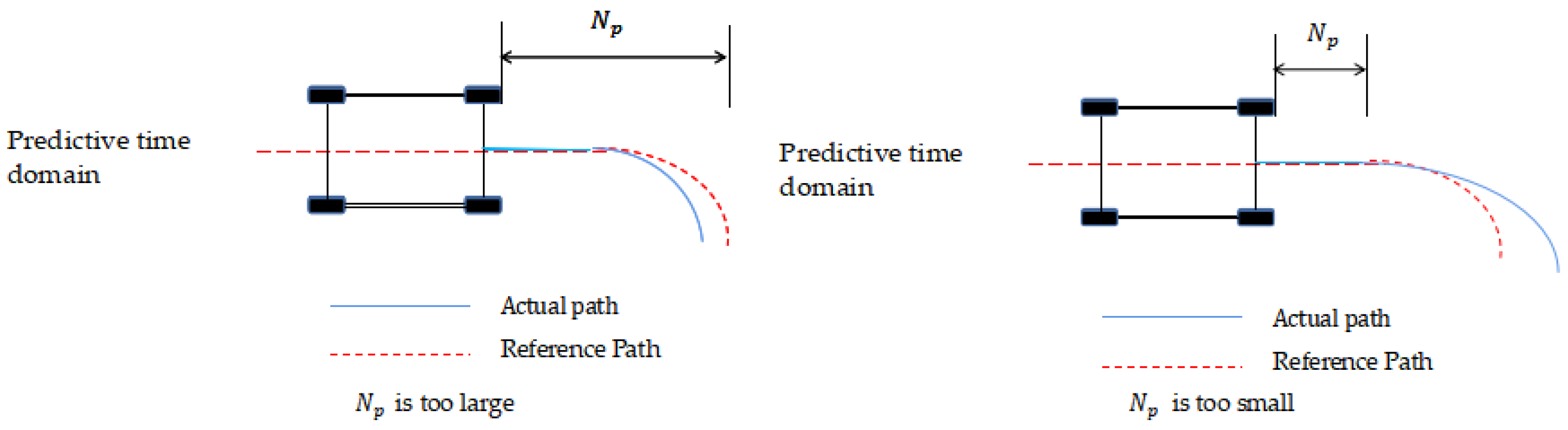
As shown in
Figure 4, when the other control parameters remain unchanged, the larger the prediction time domain is, the larger the range predicted by the controller, which can obtain more lawn mower state information. However, if the prediction time domain is too large, it will increase the error of the lawn mower at a distant position, thereby reducing the tracking accuracy of the lawn mower at a nearby position [
23]. In addition, an excessively large prediction time domain will also increase the computational complexity of the MPC algorithm and reduce the real-time performance of the system [
24]. When the prediction time domain is too small, the status information of the lawn mower will decrease. In the presence of system control constraints, the lawn mower will be unable to turn in a timely manner, the path-tracking accuracy will be reduced, and stability will not be ensured.
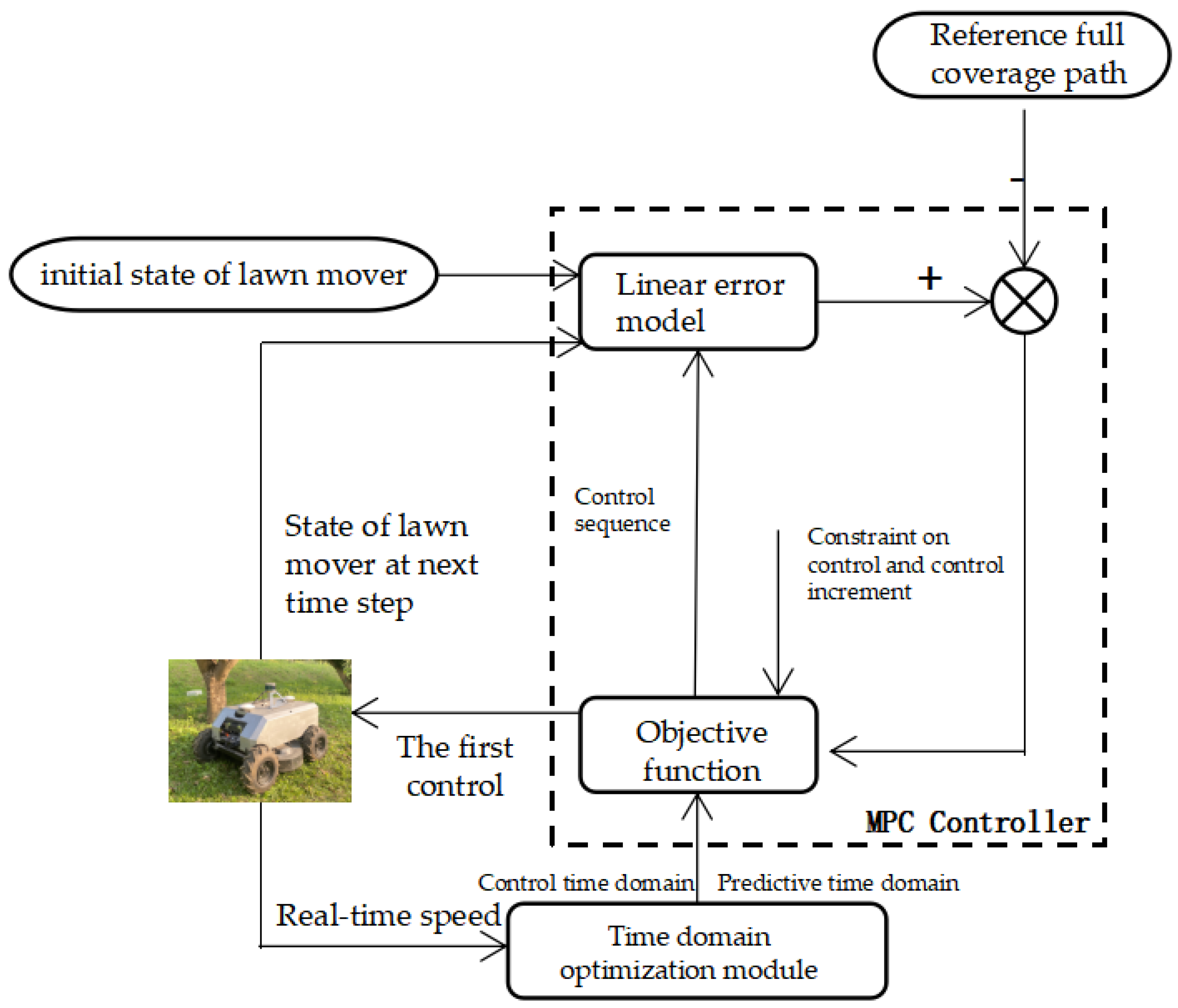
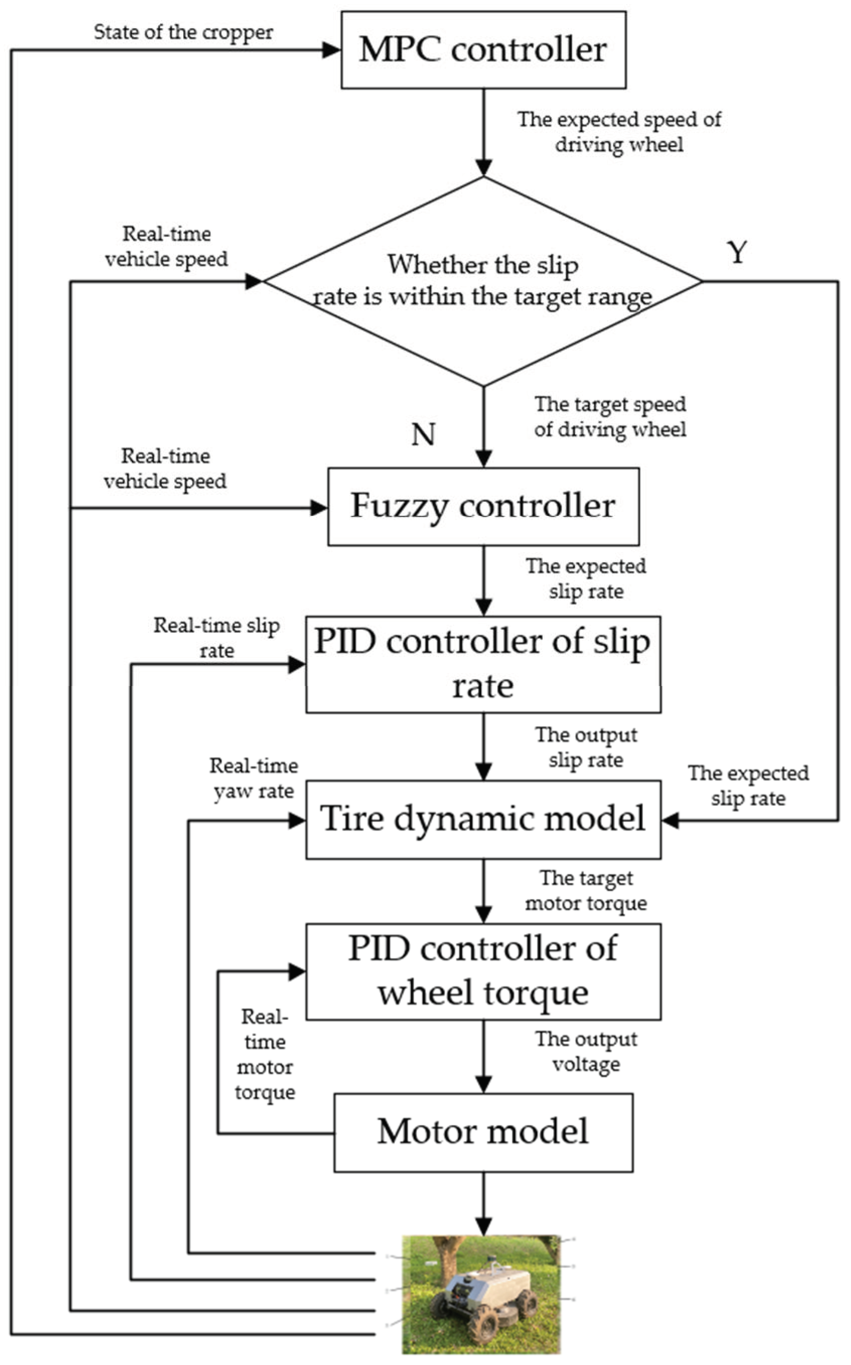
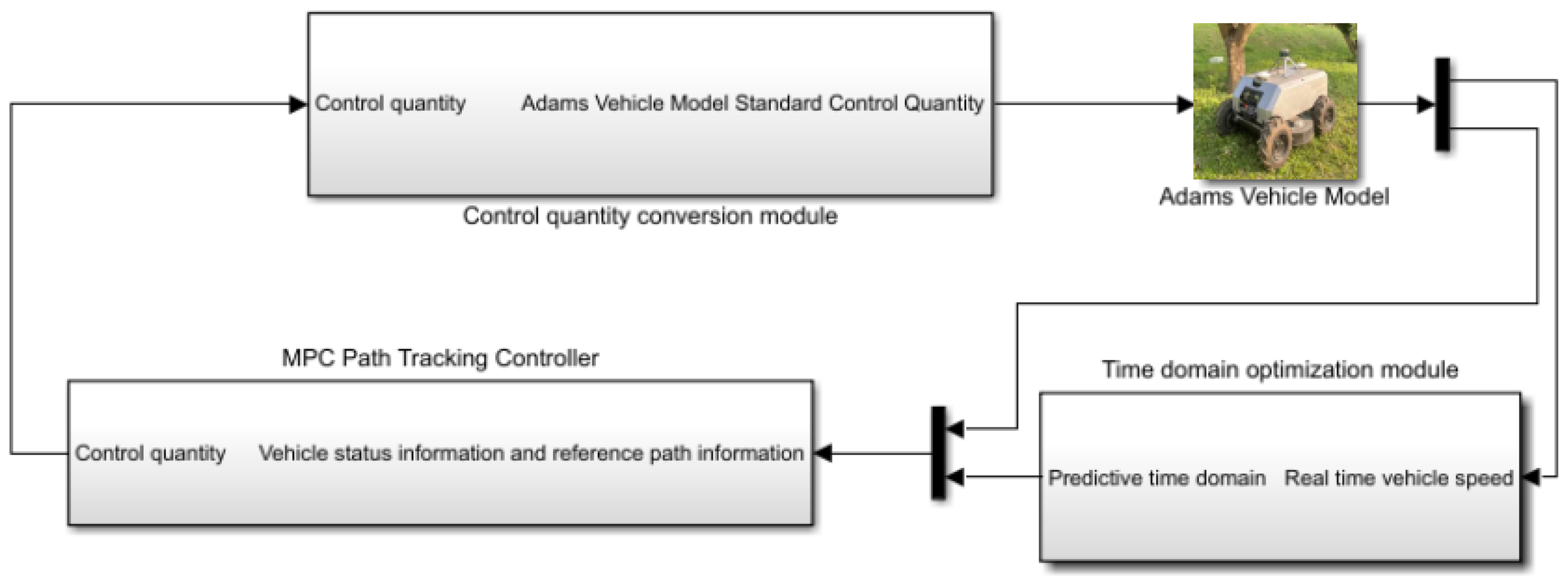
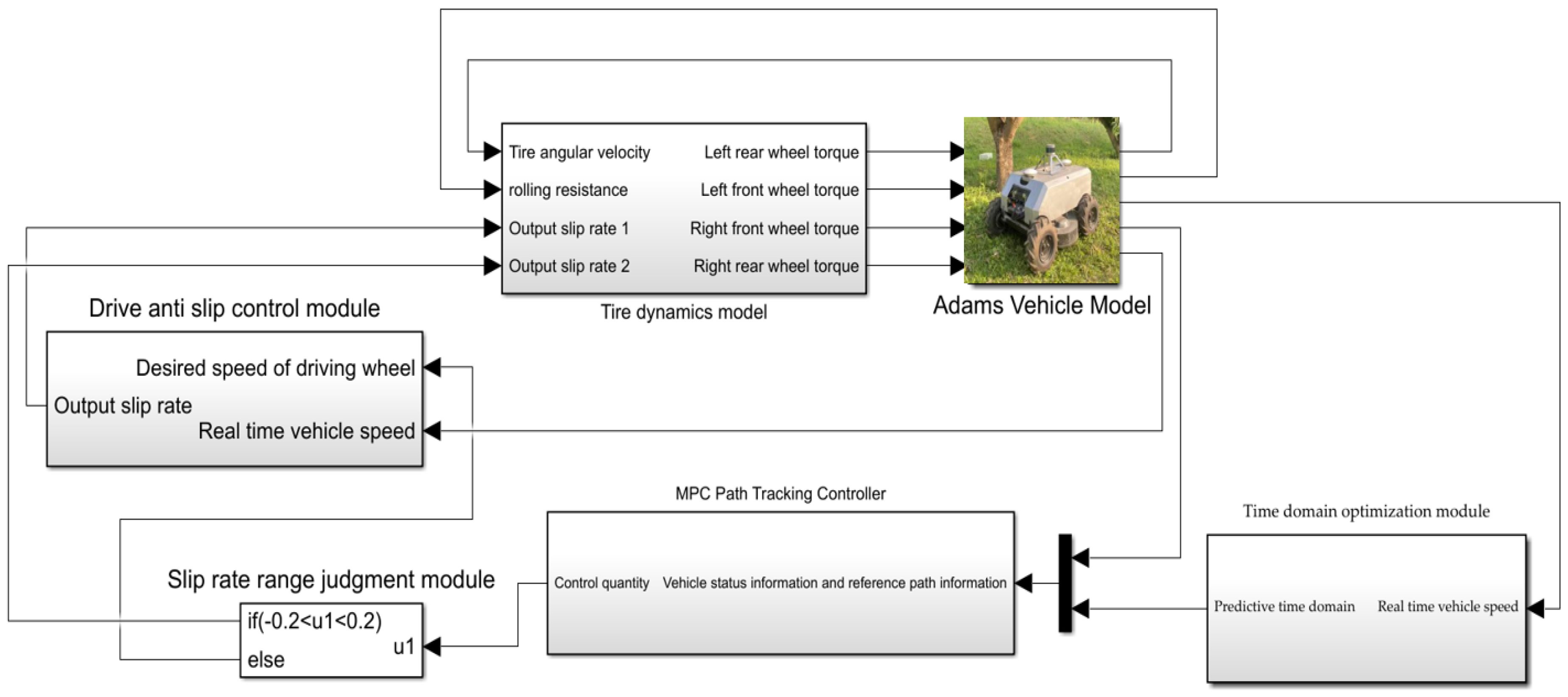
Based on the model predictive controller set above, in this section, a control time domain and prediction time domain optimization module is designed based on the vehicle’s speed, as shown in
Figure 5, to achieve adaptive parameter adjustment, improve the adaptability of the mower to environmental changes, and improve the path-tracking accuracy of the mower.
As the vehicle speed increases, the distance predicted by the MPC controller also needs to increase accordingly; that is, the predicted time domain,
, increases accordingly to ensure the stable tracking of the reference path by the lawn mower and to avoid the untimely turning phenomenon. For the control time domain,
, an increase in
can reduce the degree of sudden change in the control quantity and prevent the vehicle from slipping or even losing control during high-speed driving [
25]. Therefore, the control time domain should also increase appropriately with increasing vehicle speed to ensure the stability of path tracking.
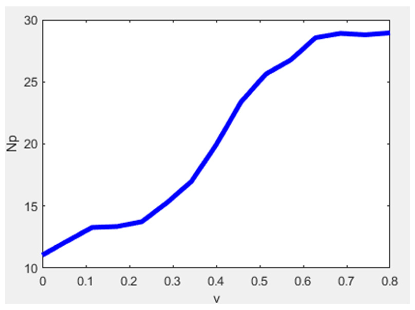
As shown in the
Figure 5, a time domain optimization module based on vehicle speed is designed using a fuzzy control algorithm. The design input is the current speed of the lawn mower, and the predicted time domain is the output. Based on the motor performance of the lawn mower, the input walking speed range of the lawn mower is determined to be [0, 0.8 m/s], and the adaptive predicted time domain value range for the reference path combined with the control algorithm is [10, 30].
The speed and prediction time domain of the lawn mower is divided into the following seven fuzzy subsets: NB (very small), NM (small), NS (small), Z (moderate), PS (large), PM (large), and PB (large). The membership function selects the Gaussian and trigonometric functions.
Based on the time domain optimization design and multiple simulation experiments, specific fuzzy rules are formulated, as shown in
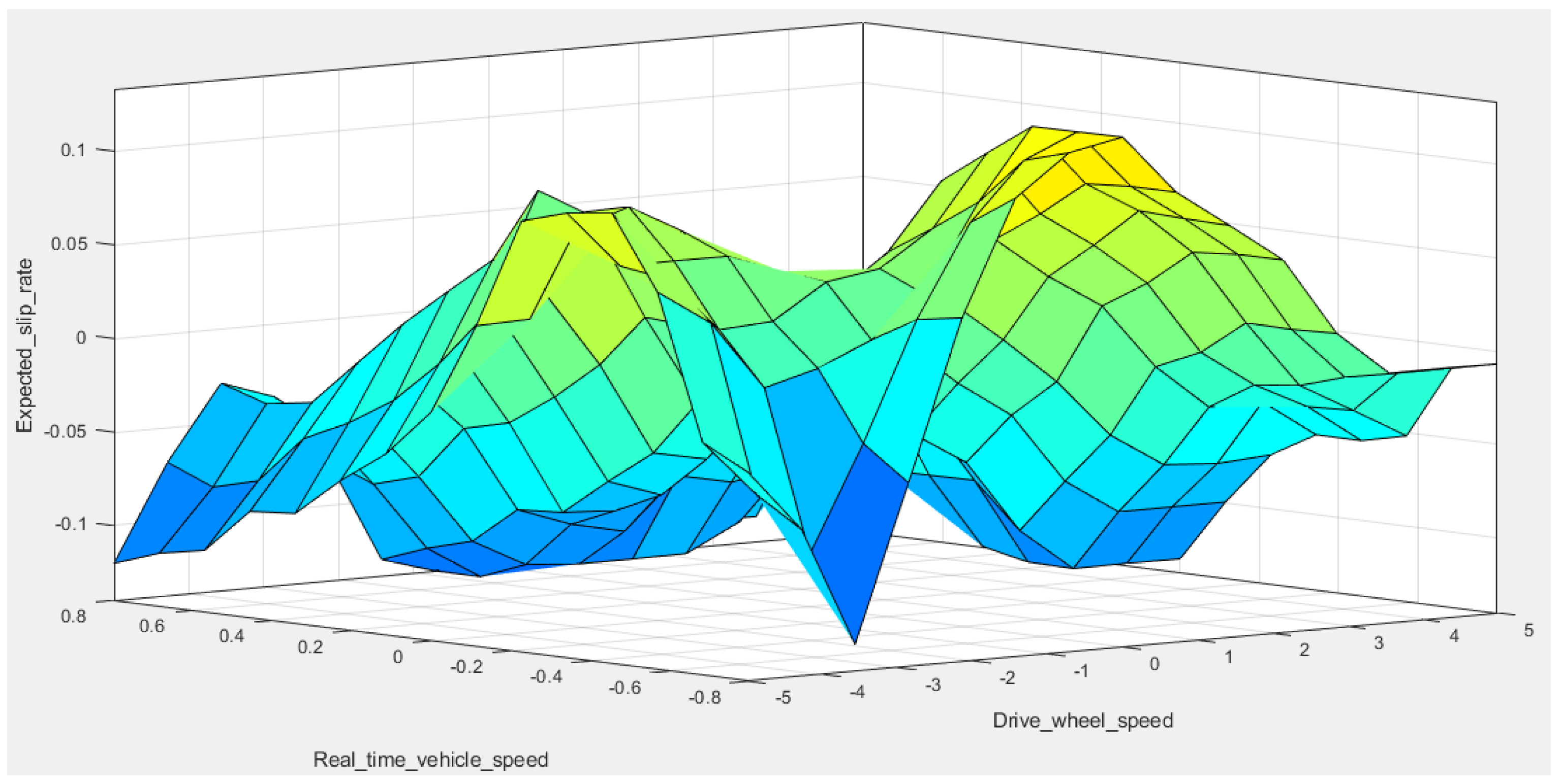
Table 2. The response relationship between the operating speed of the lawn mower and the predicted time domain is shown in
Figure 6. The operating speed of the lawn mower is obtained through fuzzy inference to determine the predicted fuzzy output in the time domain. The centroid method is selected to solve the ambiguity of this problem and obtain an accurate output prediction in the time domain.
The prediction time domain output is smoothed by the fuzzy algorithm to obtain the current optimal prediction time domain,
, after fuzzy processing. The current optimal prediction time domain is appropriately adjusted to obtain the current optimal control time domain,
The expressions for
and
are as follows:
In the above equation, is a time domain weight parameter, which usually ranges from 0.15 to 0.2. Here, based on the simulation situation, the time domain weight coefficient is selected as 0.2.


 ,
, 


