Abstract
Visible and near-infrared (vis-NIR) spectroscopy has proven to be a straightforward method for sample preparation and scaling soil testing, while the increasing availability of high-resolution remote sensing (RS) data has further facilitated the understanding of spatial variability in soil organic carbon (SOC) and total nitrogen (TN) across landscapes. However, the impact of combining vis-NIR spectroscopy with high-resolution RS data for SOC and TN prediction remains an open question. This study evaluated the effects of incorporating a high-resolution LiDAR-derived digital elevation model (DEM) and a medium-resolution SRTM-derived DEM with vis-NIR spectroscopy for predicting SOC and TN in peatlands. A total of 57 soil cores, comprising 262 samples from various horizons (<2 m), were collected and analysed for SOC and TN content using traditional methods and ASD Fieldspec® 4. The 262 observations, along with elevation data from LiDAR and SRTM, were divided into 80% training and 20% testing datasets. By employing the Cubist modelling approach, the results demonstrated that incorporating high-resolution LiDAR data with vis-NIR spectra improved predictions of SOC (RMSE: 4.60%, RPIQ: 9.00) and TN (RMSE: 3.06 g kg−1, RPIQ: 7.05). In conclusion, the integration of LiDAR and soil spectroscopy holds significant potential for enhancing soil mapping and promoting sustainable soil management.
1. Introduction
Soil organic carbon (SOC) and total nitrogen (TN) play a key role in the global biogeochemical cycle, which is important for life, with peatland soils being one of the largest terrestrial pools of carbon and nitrogen [1]. Understanding the distribution of SOC and TN in peatlands is crucial for effective peatland management, carbon accounting, and climate change mitigation. Quantifying SOC and TN is essential for determining soil quality and proposing a viable monitoring, reporting, and verification program for low-carbon agriculture [2]. Moreover, accurate estimation of SOC and TN in peatlands is essential for understanding carbon dynamics and guiding sustainable management practices. However, the challenge faced by soil scientists today is that current methods of SOC and TN measurements are expensive and time-consuming. Additionally, the demand for SOC and TN data is not met by the existing information from legacy soil data [3]. This highlights the importance of a more direct, rapid, and cost-effective method of quantifying SOC and TN.
Conventional laboratory methods of soil analysis involve the use of chemical reagents and complex laboratory equipment [4]. Furthermore, conventional laboratory soil analysis is not feasible due to its complexity, high costs, and time requirements. In contrast, simple sample preparation and time-efficient methods, such as visible (vis, 350–780 nm) and near-infrared (NIR, 780–2500 nm) spectroscopy, have been proven effective over the past four decades, allowing users to reduce the cost per test [5,6]. Vis-NIR spectroscopy provides valuable information by analysing the interaction between electromagnetic energy and matter, specifically in the case of soil. The broad and overlapping bands observed in vis-NIR spectra offer insights into the presence of organic and inorganic materials in soils, including chromophores; iron minerals; overtones of OH, CO3, and SO4 groups; as well as combinations of CO2 and H2O [4,5].
Essentially, the spectral information obtained from vis-NIR spectroscopy can be utilised to model soil properties because the spectral bands or wavelengths, which act as multiple independent variables, have an impact on the soil properties, which are the dependent variables [5]. Therefore, the spectral information is mathematically pre-processed to minimise errors associated with stray light during measurement and atmospheric water content. These spectral data are then correlated with soil properties using a range of machine learning techniques to quantify (i.e., predict or estimate) these soil properties. Despite variations in soil type, number of soil samples, pre-processing techniques, and model validation methods, several studies have demonstrated that SOC and TN in soils can be effectively modelled by applying vis-NIR spectroscopy with machine learning methods [4,7,8,9]. For instance, Cubist regression is a popular and high-performing machine learning technique for vis-NIR spectroscopy [5,10,11]. This rule-based regression model constructs a regression tree in which the final nodes contain linear models instead of discrete values. If the regression trees in each rule/node are satisfied by the input variables, the rules’ instances pass a multivariate linear regression model. This feature makes Cubist regression a readable “if-then” conditional statement, as highlighted by Viscarra-Rossel et al. [5].
Alongside diffuse reflectance spectroscopy, the growing availability of remotely sensed data provides opportunities to enhance understanding of the spatially heterogeneous high variability of SOC and TN in the landscape. These remote sensing data are utilised as environmental variables (i.e., predictors or covariates) that can enhance the interpretability of soil predictions in a highly heterogeneous landscape [12]. Numerous studies in soil science have demonstrated satisfactory accuracy in predicting soil properties (e.g., SOC and TN) using high-resolution digital elevation models (DEM) (i.e., LiDAR) and terrain derivatives as environmental variables [13,14,15,16,17,18].
The integration of soil spectroscopy with remote sensing data has gained significant attention in soil science research in recent years [12,19,20]. This combination offers the potential to enhance our understanding of soil properties and processes at large scales, providing valuable insights for land management and environmental sustainability. However, like any scientific approach, it comes with its own set of advantages and disadvantages. Integrating soil spectroscopy with remote sensing data can significantly reduce the cost and time required for traditional soil sampling and laboratory analysis. It offers a rapid and cost-effective means of obtaining soil information, making it feasible for large-scale soil mapping and monitoring projects. A disadvantage is that while remote sensing data provide broad-scale coverage, the spatial resolution may not be sufficient to capture fine-scale soil variations, particularly in heterogeneous landscapes. This limitation can hinder the accurate characterisation of small-scale soil features and local variability.
Few studies have assessed the impacts of combining diffuse reflectance spectroscopy with high-resolution environmental variables (i.e., DEM derivatives) for SOC and TN prediction [12,19,20]. The most recent work to address this issue [12] concluded that further research should be undertaken to evaluate the use of LiDAR technology to derive a very high-resolution DEM. Additionally, the authors stated that a very high-resolution DEM has the potential to enhance the prediction of soil properties by detecting fine-scale terrain variations. In this study, we examine the advantages and disadvantages of integrating vis-NIR spectroscopy with remote sensing data. Therefore, we assessed the effects of: (i) high-resolution DEM derived from LiDAR and (ii) medium-resolution DEM derived from SRTM in combination with vis-NIR spectroscopy for SOC and TN prediction in peatlands. To determine the potential contribution of these environmental variables, the prediction of SOC and TN was performed solely using the vis-NIR spectral data as a benchmark.
2. Materials and Methods
2.1. Study Area and Soil Samples
The main type of wetland in the study area is peatland, with an average groundwater level of up to 0.3 m depth, a mean annual temperature of 9.5 °C, and a mean annual precipitation of 550 mm. The landscape relief has an amplitude of 14 m, predominantly consisting of flat terrain, which further contributes to the formation of groundwater-dependent ecosystems. Additionally, the interaction between biomass, water table, and nutrient cycling in peatlands controls the formation of microrelief forms, resulting in significant heterogeneity in soil organic matter content. The most common soil groups in the study area, according to the World Reference Base soil classification [21], are Arenosols, Gleysols, and Histosols, all of which hold particular importance in peatland ecosystems. Arenosols are characterised by sandy textures and low organic matter content and can be found in transitional areas between mineral soil and peat deposits within peatlands. Gleysols exhibit gleyic properties, characterised by waterlogging and poor drainage due to restricted drainage conditions. In peatlands, Gleysols often occur in areas with high water tables, where water movement is hindered by peat accumulation or other factors such as topography. Histosols are organic soils with a high proportion of organic matter, primarily derived from partially decomposed plant material. In peatlands, Histosols are dominant and represent the organic-rich layers that constitute peat deposits.
The soil sampling design followed a stratified random sampling method, as described in [18], and involved a total of 57 soil cores, resulting in 262 samples (Figure 1). A hydraulic probe with a length of 2 m and a diameter of 10 cm was used to collect these soil cores. It is important to note that the soil cores were divided into horizons, resulting in variations in depths across the samples. Afterwards, the 262 soil samples were air-dried, ground, and sieved through a <2 mm mesh size before being sent for conventional laboratory and spectral analyses.
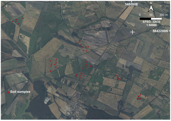
Figure 1.
Study area and spatial distribution of the soil cores.
2.2. Conventional Laboratory Analysis of Soil Organic Carbon and Total Nitrogen
The soil samples were first air-dried and sieved to obtain the <2 mm fraction. Subsequently, an aliquot of this fraction was oven-dried at 105 °C for 24 h. The determination of total carbon (C) and nitrogen (N) content was carried out using elemental analysis (CNS analyser TruSpec, LECO Ltd., Mönchengladbach, Germany) through dry combustion at 1250 °C (DIN ISO 10694, 1996 [22]; DIN ISO 13878, 1998 [23]). Carbonate C was determined using gas chromatographic analysis of carbon dioxide evolution (Carmograph by Woesthoff, Scheibler-method) after the application of phosphoric acid. The soil organic carbon content (SOC, wt. %) was calculated by subtracting the carbonate C from the total C. All data are reported on an oven-dry basis.
2.3. Visible and Near-Infrared Soil Spectral Library
Prior to vis-NIR analysis, the 262 samples were air-dried (45 °C for 48 h), ground, and sieved (<2 mm mesh). Approximately 12 g of each soil sample was placed uniformly in Petri dishes. The vis-NIR spectral data of the soil samples were measured in a dark laboratory room using an ASD Fieldspec® 4 spectroradiometer (Boulder, CO, USA). The spectroradiometer had a spectral range of 350–2500 nm and a sampling interval of 1 nm, with a resolution of 1 nm from 350 to 700 nm, 3 nm from 700 to 1400 nm, and 10 nm from 1400 to 2500 nm. All vis-NIR spectra were collected using a standard contract probe in three replications. Each spectrum was an average of 10 scans taken at the centre of the samples, with a radius of 5 mm. The probe included an optical fibre and a halogen bulb light source (2901 ± 10 K) to minimise errors due to stray light and atmospheric water content. Prior to recording the spectra of each soil sample, the ASD Fieldspec 4 spectroradiometer was optimised on a dark current and a standard white reference panel (Spectralon®). The spectral interval was narrowed to 400–2380 nm to exclude noisy regions of the vis-NIR spectra, resulting in 1981 spectral bands. Following the approach by Mendes et al. [24], each spectrum was corrected using a spline correction method with the “prospectr” R package, and no further pre-processing procedure was necessary.
2.4. Environmental Variables from Remote Sensing
The environmental variables were derived from two sets of elevation data with original spatial resolutions of 1 m and 30 m. The first set was obtained from a high-resolution Light Detection and Ranging (LiDAR) flyover conducted in December 2008, resulting in 1 × 1 m digital elevation model (DEM) raster dataset. The LiDAR flyover captured four points per square metre at a pulse frequency of 50,000 Hz, with a vertical accuracy of 3 cm. The second set of elevation data were sourced from the Shuttle Radar Topography Mission [25], providing a 30 m DEM raster dataset. These two DEMs are referred to as DEMLiDAR_1m and DEMSRTM_30m, respectively. To ensure a fair comparison, the DEMLiDAR_1m dataset was resampled to a 30 m spatial resolution (DEMLiDAR_30m) (Figure 2). QGIS software was used to calculate three terrain derivatives, slope, topographic wetness index (TWI), and topographic position index (TPI; [26]), from the three DEM datasets. A summary of the four environmental variables is presented in Table 1.
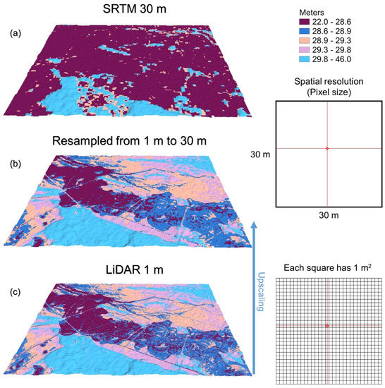
Figure 2.
Digital elevation models from SRTM (a), LiDAR resampling procedure (b), and LiDAR (c) in the study area.

Table 1.
List of environmental variables.
2.5. Modelling Procedures and Model Assessment
The 262 observations were divided using conditioned Latin Hypercube Sampling (cLHS; [27]): 80% (209 samples) for training the prediction model and 20% (53 samples) for testing accuracy. The R package “clhs” [28] was utilised to select cLHS samples based on vis-NIR spectra. An R implementation of Cubist [10,11], a rule-based regression model, was employed for training the prediction models. The regression tree constructed by Cubist included linear models in its final nodes. If input variables satisfied the regression trees in each rule/node, the rule instances passed a multivariate linear regression model. The default hyperparameter settings, such as the neighbours, number of committees, and rules, were used for the Cubist models. The default parameters were selected using the training data and a 10-fold cross-validation method implemented through the R package “caret” [29].
Model validation and performance were evaluated using the testing data, with assessment parameters including root mean square error (1), model efficiency coefficient [30] (2), bias (3), and concordance Lin’s correlation coefficient (4).
where , , , , , , , and are, respectively, the sample sizes, observed values, predicted values of the response variable, the prediction and observation variances, the means of the predicted and observed values, and the correlation coefficient between the predicted and observed values.
3. Results
3.1. Exploratory Data Analysis of Soil Organic Carbon and Total Nitrogen
The descriptive statistics are presented in Figure 3, summarising the range of SOC (0.03–55.64%) and TN (0.05–33.21 g kg−1) values. The considerable variation observed in SOC and TN can be attributed to the sampling of peatland soils, ensuring a robust characterisation. The skewness values of approximately 0.5 indicate a nearly symmetrical normal distribution for both SOC and TN, facilitating the optimal fitting of regression models in the training dataset.
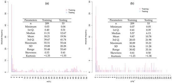
Figure 3.
Summary statistics of training and testing datasets of soil organic carbon (a) and total nitrogen (b).
3.2. Relationship between vis-NIR Spectra and Soil Components
The broad and overlapping bands in the vis-NIR spectra pose challenges for interpretation, due to the limited absorption features in the vis-NIR spectral data of soil samples (Figure 4). Nonetheless, useful information about organic and inorganic materials in soils can still be inferred from chromophores [31] and iron minerals [32] in the visible spectral region (400–700 nm). In the NIR spectral region (400–700 nm), absorption features can be associated with overtones of hydroxyl (OH−), carbonate (CO32−), and sulphate (SO42−) groups, as well as combinations of fundamental features of carbon dioxide (CO2) and water (H2O) [31,32]. Furthermore, diagnostic bands in the vis-NIR spectra can facilitate the detection of clay minerals (e.g., kaolinite: ~2080–~2270 nm and smectite: ~2120–~2290 nm), iron oxides (e.g., goethite: ~415 and ~445 nm and hematite: ~535 and ~580 nm), organic carbon (~600, ~1910, and ~2100 nm), and carbonates (~2300–~2350 nm) [33].
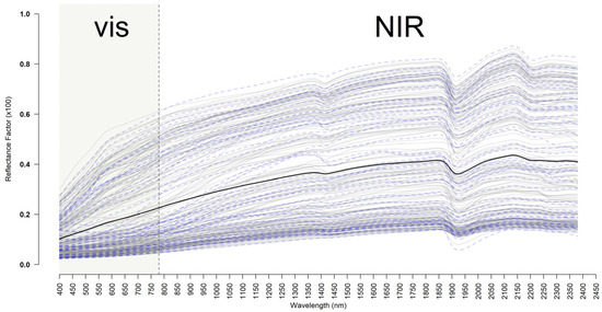
Figure 4.
Spectral curves of the training (grey line) and testing (blue line) datasets in the visible (vis) and near-infrared (NIR) ranges. Black line represents the mean values of all spectral data.
3.3. Effects of Environmental Variables on Model Prediction
Table 2 shows the performance of the Cubist model in predicting SOC using only vis-NIR spectra (benchmark) and incorporating environmental variables at 1 m and 30 m spatial resolutions along with vis-NIR spectra. Overall, the best accuracies were achieved by combining vis-NIR spectral data with high-resolution environmental variables obtained from LiDAR and resampled LiDAR. However, the models incorporating terrain data exhibited slightly better performance than the benchmark. The model using vis-NIR spectra and LiDAR demonstrated the lowest bias compared with the model using resampled LiDAR, as well as a lower RMSE compared with the benchmark. In contrast, the inclusion of coarse environmental variables from SRTM did not enhance SOC prediction and yielded the poorest indices.
Table 2.
The effect of incorporating environmental variables into vis-NIR spectral data for SOC prediction (%).
The impact of merging spectral data and environmental variables obtained from LiDAR, resampled LiDAR, and SRTM on TN predictions is presented in Table 3. The combination of LiDAR-derived environmental variables with vis-NIR spectral data demonstrated the most favourable model evaluation parameters for TN prediction, yielding an RMSE of 3.06 g kg−1 and an RPIQ of 7.05. Among the validation metrics employed, RMSE, Bias, and RPIQ exhibited subtle variations across the models, indicating their sensitivity in assessing model performance.
Table 3.
The effect of incorporating environmental variables with vis-NIR spectral data for TN prediction (g kg−1).
4. Discussion
Although the soil samples were obtained from a severely degraded peatland, the SOC and TN contents exhibited significant variability. This observation is important because SOC, for example, plays a crucial role in C balance [17,18]. The quality and representativeness of SOC and TN contents are critical for modelling, as they introduce inherent variability. In addition, it is uncommon to find a naturally occurring normal distribution in a soil dataset [34], but in our study, we observed a nearly symmetrical normal distribution for both SOC and TN.
The broad and overlapping bands in the vis-NIR spectra make them challenging to interpret, primarily because the vis-NIR spectral data of soil samples have fewer absorption features. Nevertheless, valuable information about organic and inorganic materials in soils can be linked to chromophores and iron minerals in the visible spectral region. The overtones of OH, CO3, and SO4 groups, as well as combinations of CO2 and H2O, can be associated with absorption features in the NIR spectral region [7,35]. Since the vis-NIR spectral data retrieve the signals associated with the soil mineral-organic matrix, spectroscopic modelling can reasonably estimate the concentration of SOC and TN. Examples of the effectiveness of the vis-NIR spectral model can be found in studies dating from 1991 [6] to the present [4,36].
In this study, the model evaluation was conducted using an independent test dataset of 53 observations, which avoids overly optimistic conclusions. As a benchmark to determine the potential contribution of the environmental variables derived from LiDAR and SRTM, the prediction of SOC and TN was performed using the vis-NIR spectral data alone. The results are consistent with previous studies on SOC and TN [24,37,38,39,40]. For example, successful SOC predictions were obtained, with R2 values ranging from 0.64 to 0.96. Similarly, TN was predicted quite accurately, with R2 values ranging from 0.48 to 0.94.
SOC and TN in degraded peatland soils are strongly influenced by topographic changes from micro-highs to micro-lows, which can be determined using, for example, a high resolution topographic position index [18]. The results demonstrate that SOC (RMSE: 4.60%, MEC: 0.94, CCC: 0.95, Bias: 0.04, and RPIQ: 9.00) and TN (RMSE: 3.06 g kg−1, MEC: 0.92, CCC: 0.94, Bias: −0.52, and RPIQ: 7.05) can be accurately predicted by incorporating high-resolution terrain data derived from LiDAR using Cubist. The RMSE decreased by 5% and 3% for SOC and TN, respectively, compared with the model using only vis-NIR spectra. Incorporating coarse environmental variables from SRTM with spectral data did not improve SOC prediction and displayed the worst indices. Sabetizade et al. [12] suggested that the combination of fine-scale terrain remote sensing data with diffuse reflectance spectroscopy should be tested as these remote sensing data become more widely available. Therefore, our results have demonstrated that a very high-resolution DEM could potentially improve the prediction of soil properties by detecting fine-scale terrain variations. Integrating vis-NIR spectroscopy with LiDAR and SRTM data allows for the incorporation of both spectral and spatial information, resulting in more accurate models for predicting SOC and TN in peatlands.
Perhaps, just as importantly, we should point out the difference between LiDAR and SRTM, as it explains why a very high-resolution DEM yielded better results in our study. LiDAR is an active remote sensing technology that measures distances by illuminating a target with laser pulses and analysing the reflected signals. It provides high-resolution (e.g., 1 m resolution) three-dimensional information about the Earth’s surface, including vegetation height, canopy structure, and terrain elevation. LiDAR data acquisition is typically conducted using airborne or terrestrial platforms, allowing for flexible coverage and varying spatial resolutions. The high-resolution point cloud data generated by LiDAR can be integrated with soil spectroscopy to improve soil property estimation, such as organic matter content, moisture content, and compaction.
On the other hand, SRTM is a spaceborne radar mission that aims to provide global digital elevation models (DEMs) with medium spatial resolution. It uses synthetic aperture radar (SAR) to measure surface topography and generates DEMs with a resolution of approximately 30 m. SRTM data, readily available for large-scale studies, offer valuable information on terrain characteristics and slope, which are essential factors influencing soil distribution (e.g., SOC and TN). However, the coarse spatial resolution of SRTM limits its direct use for detailed soil mapping.
As we have demonstrated through our results, vis-NIR spectroscopy, when combined with LiDAR or SRTM data, enables the development of predictive models to estimate SOC and TN across different spatial scales. The integration of LiDAR, SRTM, and vis-NIR spectroscopy enhances the spatial resolution capabilities. The integration of these data sources improves the overall accuracy of soil analysis, and these technologies offer a comprehensive approach to enhance the spatial resolution and accuracy of soil property mapping in peatland environments. Some limitations and challenges should also be addressed when evaluating our results and considering the spatial co-registration, data availability, and scale effects of LiDAR, SRTM, and soil spectroscopy (e.g., vis-NIR). Integrating LiDAR, SRTM, and soil spectroscopy datasets requires precise spatial co-registration to ensure accurate alignment of the different data layers. Misalignments can introduce errors in the integrated analysis, leading to inaccuracies in soil property estimation. Secondly, although LiDAR and SRTM datasets are increasingly accessible, their availability can still be limited in certain regions, particularly in developing countries or remote areas. Adequate data coverage is necessary to ensure the effectiveness of the integration approach. Last but not least, the integration of LiDAR, SRTM, and soil spectroscopy data is subject to scale effects. Different soil properties exhibit spatial variations at various scales, and capturing these variations accurately requires careful consideration of the spatial resolution and extent of the integrated datasets.
5. Conclusions
Regarding our results, we were able to address the research question concerning the effects of combining vis-NIR spectroscopy with high-resolution environmental variables (i.e., DEM derivatives) for predicting SOC and TN. Therefore, in this study, we evaluated the combination of vis-NIR spectra with high-resolution DEM derived from LiDAR and medium-resolution DEM derived from SRTM for the prediction of SOC and TN in peatlands. The addition of high-resolution DEM and terrain derivatives resulted in a slight improvement in the prediction of SOC and TN. Undoubtedly, the best models for predicting SOC and TN are still those that solely utilise the vis-NIR spectra. However, this study has demonstrated the relevance of vis-NIR spectroscopy in conjunction with high resolution terrain data in enhancing the spatial estimation of TN and SOC.
The integration of LiDAR and SRTM with soil spectroscopy presents a promising approach to enhance soil mapping and analysis. By combining high-resolution vertical information, terrain characteristics, and detailed soil property data, researchers and land managers can gain valuable insights into soil variability across different scales. Additionally, the integration of digital elevation data helps identify landscape units that are associated with distinct SOC and TN characteristics, enabling a more comprehensive understanding of peatland dynamics. Despite certain limitations and challenges, this integration offers significant potential for improving precision agriculture, land management practices, and environmental monitoring, contributing to sustainable soil resource management. By combining existing datasets and leveraging advanced modelling techniques, researchers can achieve accurate predictions of SOC and TN without extensive field campaigns, thereby reducing costs and saving time [41].
Author Contributions
Conceptualisation, W.d.S.M.; methodology, W.d.S.M. and M.S.; software, W.d.S.M.; validation, W.d.S.M.; formal analysis, W.d.S.M.; investigation, W.d.S.M.; resources, M.S.; data curation, W.d.S.M.; writing—original draft preparation, W.d.S.M.; writing—review and editing, W.d.S.M. and M.S.; visualisation, W.d.S.M. All authors have read and agreed to the published version of the manuscript.
Funding
Funding for this study was provided by the German Federal Ministry of Education and Research (BMBF, project: “Climate protection by peatland protection—Strategies for peatland management”, 01LS05049).
Data Availability Statement
The vis-NIR soil spectral data are not publicly available.
Acknowledgments
We would like to thank Ingrid Onasch for technical assistance in carrying out the vis-NIR measurements on the soil samples.
Conflicts of Interest
The authors declare no conflict of interest and the funders had no role in the design of the study; in the collection, analyses, or interpretation of data; in the writing of the manuscript; or in the decision to publish the results.
References
- Batjes, N.H. Total carbon and nitrogen in the soils of the world. Eur. J. Soil Sci. 1996, 47, 151–163. [Google Scholar] [CrossRef]
- Norse, D. Low carbon agriculture: Objectives and policy pathways. Environ. Dev. 2012, 1, 25–39. [Google Scholar] [CrossRef]
- McBratney, A.B.; Minasny, B.; Viscarra Rossel, R. Spectral soil analysis and inference systems: A powerful combination for solving the soil data crisis. Geoderma 2006, 136, 272–278. [Google Scholar] [CrossRef]
- Barra, I.; Haefele, S.M.; Sakrabani, R.; Kebede, F. Soil spectroscopy with the use of chemometrics, machine learning and pre-processing techniques in soil diagnosis: Recent advances–A review. TrAC—Trends Anal. Chem. 2021, 135, 116166. [Google Scholar] [CrossRef]
- Viscarra Rossel, R.A.; Behrens, T.; Ben-Dor, E.; Chabrillat, S.; Demattê, J.A.M.; Ge, Y.; Gomez, C.; Guerrero, C.; Peng, Y.; Ramirez-Lopez, L.; et al. Diffuse reflectance spectroscopy for estimating soil properties: A technology for the 21st century. Eur. J. Soil Sci. 2022, 73, e13271. [Google Scholar] [CrossRef]
- Shonk, J.L.; Gaultney, L.D.; Schulze, D.G.; Van Scoyoc, G.E. Spectroscopic Sensing of Soil Organic Matter Content. Trans. ASAE 1991, 34, 1978–1984. [Google Scholar] [CrossRef]
- Demattê, J.A.M.; Dotto, A.C.; Paiva, A.F.S.; Sato, M.V.; Dalmolin, R.S.D.; de Araújo, M.d.S.B.; da Silva, E.B.; Nanni, M.R.; ten Caten, A.; Noronha, N.C.; et al. The Brazilian Soil Spectral Library (BSSL): A general view, application and challenges. Geoderma 2019, 354, 113793. [Google Scholar] [CrossRef]
- Ng, W.; Minasny, B.; de Mendes, W.S.; Demattê, J.A.M. The influence of training sample size on the accuracy of deep learning models for the prediction of soil properties with near-infrared spectroscopy data. SOIL 2020, 6, 565–578. [Google Scholar] [CrossRef]
- Soriano-Disla, J.M.; Janik, L.J.; Viscarra Rossel, R.A.; Macdonald, L.M.; McLaughlin, M.J. The Performance of Visible, Near-, and Mid-Infrared Reflectance Spectroscopy for Prediction of Soil Physical, Chemical, and Biological Properties. Appl. Spectrosc. Rev. 2014, 49, 139–186. [Google Scholar] [CrossRef]
- Kuhn, M.; Quinlan, R. Cubist: Rule-and Instance-Based Regression Modeling. Available online: https://cran.r-project.org/web/packages/Cubist/index.html (accessed on 3 December 2020).
- Quinlan, J.R. C4.5; Elsevier: Amsterdam, The Netherlands, 1993; ISBN 9780080500584. [Google Scholar]
- Sabetizade, M.; Gorji, M.; Roudier, P.; Zolfaghari, A.A.; Keshavarzi, A. Combination of MIR spectroscopy and environmental covariates to predict soil organic carbon in a semi-arid region. Catena 2021, 196, 104844. [Google Scholar] [CrossRef]
- Guo, Z.; Adhikari, K.; Chellasamy, M.; Greve, M.B.; Owens, P.R.; Greve, M.H. Selection of terrain attributes and its scale dependency on soil organic carbon prediction. Geoderma 2019, 340, 303–312. [Google Scholar] [CrossRef]
- Gatis, N.; Luscombe, D.J.; Carless, D.; Parry, L.E.; Fyfe, R.M.; Harrod, T.R.; Brazier, R.E.; Anderson, K. Mapping upland peat depth using airborne radiometric and lidar survey data. Geoderma 2019, 335, 78–87. [Google Scholar] [CrossRef]
- Mulder, V.L.L.; De Bruin, S.; Schaepman, M.E.E.; Mayr, T.R.R. The use of remote sensing in soil and terrain mapping—A review. Geoderma 2011, 162, 1–19. [Google Scholar] [CrossRef]
- de Mendes, W.S.; Demattê, J.A.M.; Silvero, N.E.Q.; Rabelo Campos, L. Integration of multispectral and hyperspectral data to map magnetic susceptibility and soil attributes at depth: A novel framework. Geoderma 2021, 385, 114885. [Google Scholar] [CrossRef]
- Minasny, B.; Berglund, Ö.; Connolly, J.; Hedley, C.; de Vries, F.; Gimona, A.; Kempen, B.; Kidd, D.; Lilja, H.; Malone, B.; et al. Digital mapping of peatlands—A critical review. Earth-Sci. Rev. 2019, 196, 102870. [Google Scholar] [CrossRef]
- Koszinski, S.; Miller, B.A.; Hierold, W.; Haelbich, H.; Sommer, M. Spatial Modeling of Organic Carbon in Degraded Peatland Soils of Northeast Germany. Soil Sci. Soc. Am. J. 2015, 79, 1496–1508. [Google Scholar] [CrossRef]
- Vašát, R.; Kodešová, R.; Borůvka, L.; Jakšík, O.; Klement, A.; Brodský, L. Combining reflectance spectroscopy and the digital elevation model for soil oxidizable carbon estimation. Geoderma 2017, 303, 133–142. [Google Scholar] [CrossRef]
- Peng, Y.; Xiong, X.; Adhikari, K.; Knadel, M.; Grunwald, S.; Greve, M.H. Modeling soil organic carbon at regional scale by combining multi-spectral images with laboratory spectra. PLoS ONE 2015, 10, e0142295. [Google Scholar] [CrossRef] [PubMed]
- IUSS Working Group WRB. World Reference Base for Soil Resources 2014: International Soil Classification System for Naming Soils and Creating Legends for Soil Maps; FAO: Rome, Italy, 2015; ISBN 9789251083697. [Google Scholar]
- DIN ISO10694:1996-08; Bodenbeschaffenheit—Bestimmung von organischem Kohlenstoff und Gesamtkohlenstoff nach trockener Verbrennung (Elementaranalyse). Soil Quality—Determination of Organic and Total Carbon after Dry Combustion (Elementary Analysis); ISO: Berlin, Germany, 1996.
- DIN ISO 13878; Bodenbeschaffenheit—Bestimmung des Gesamt-Stickstoffs durch trockene Verbrennung (Elementaranalyse). Soil Quality e Determination of Total Nitrogen Content by Dry Combustion (Elemental Analysis); ISO: Berlin, Germany, 1998.
- Mendes, W.S.; Sommer, M.; Koszinski, S.; Wehrhan, M. Peatlands spectral data influence in global spectral modelling of soil organic carbon and total nitrogen using visible-near-infrared spectroscopy. J. Environ. Manage. 2022, 317, 115383. [Google Scholar] [CrossRef]
- USGS. USGS EROS Archive—Digital Elevation—Shuttle Radar Topography Mission (SRTM) 1 Arc-Second Global. Available online: https://www.usgs.gov/centers/eros/science/usgs-eros-archive-digital-elevation-shuttle-radar-topography-mission-srtm-1-arc?qt-science_center_objects=0#qt-science_center_objects (accessed on 29 May 2020).
- Weiss, A. Topographic position and landforms analysis. In ESRI Users Conference; The Nature Conservancy, Northwest Division: San Diego, CA, USA, 2001. [Google Scholar]
- Minasny, B.; McBratney, A.B. A conditioned Latin hypercube method for sampling in the presence of ancillary information. Comput. Geosci. 2006, 32, 1378–1388. [Google Scholar] [CrossRef]
- Roudier, P.; Hewitt, A.; Beaudette, D. A conditioned Latin hypercube sampling algorithm incorporating operational constraints. In Digital Soil Assessments and Beyond; CRC Press: Boca Raton, FL, USA, 2012; pp. 227–231. [Google Scholar]
- Kuhn, M. Building Predictive Models in R Using the caret Package. J. Stat. Softw. 2008, 28, 1–26. [Google Scholar] [CrossRef]
- Janssen, P.H.M.; Heuberger, P.S.C. Calibration of process-oriented models. Ecol. Modell. 1995, 83, 55–66. [Google Scholar] [CrossRef]
- Ben-Dor, E.; Banin, A. Visible and near-infrared (0.4–1.1 μm) analysis of arid and semiarid soils. Remote Sens. Environ. 1994, 48, 261–274. [Google Scholar] [CrossRef]
- Stoner, E.R.; Baumgardner, M.F. Characteristic Variations in Reflectance of Surface Soils. Soil Sci. Soc. Am. J. 1981, 45, 1161. [Google Scholar] [CrossRef]
- Clark, R.N.; King, T.V.V.; Klejwa, M.; Swayze, G.A.; Vergo, N. High spectral resolution reflectance spectroscopy of minerals. J. Geophys. Res. 1990, 95, 12653–12680. [Google Scholar] [CrossRef]
- Malone, B.P.; McBratney, A.B.; Minasny, B. Spatial Scaling for Digital Soil Mapping. Soil Sci. Soc. Am. J. 2013, 77, 890. [Google Scholar] [CrossRef]
- Stenberg, B.; Viscarra Rossel, R.A.; Mouazen, A.M.; Wetterlind, J. Visible and Near Infrared Spectroscopy in Soil Science. In Advances in Agronomy; Sparks, D.L., Ed.; Academic Press: Cambridge, MA, USA, 2010; Volume 107, pp. 163–215. [Google Scholar]
- Ben-Dor, E.; Banin, A. Near-Infrared Analysis as a Rapid Method to Simultaneously Evaluate Several Soil Properties. Soil Sci. Soc. Am. J. 1995, 59, 364–372. [Google Scholar] [CrossRef]
- Riedel, F.; Denk, M.; Müller, I.; Barth, N.; Gläßer, C. Prediction of soil parameters using the spectral range between 350 and 15,000 nm: A case study based on the Permanent Soil Monitoring Program in Saxony, Germany. Geoderma 2018, 315, 188–198. [Google Scholar] [CrossRef]
- Reda, R.; Saffaj, T.; Ilham, B.; Saidi, O.; Issam, K.; Brahim, L.; El Hadrami, E.M. A comparative study between a new method and other machine learning algorithms for soil organic carbon and total nitrogen prediction using near infrared spectroscopy. Chemom. Intell. Lab. Syst. 2019, 195, 103873. [Google Scholar] [CrossRef]
- Barthès, B.G.; Kouakoua, E.; Clairotte, M.; Lallemand, J.; Chapuis-Lardy, L.; Rabenarivo, M.; Roussel, S. Performance comparison between a miniaturized and a conventional near infrared reflectance (NIR) spectrometer for characterizing soil carbon and nitrogen. Geoderma 2019, 338, 422–429. [Google Scholar] [CrossRef]
- Tsakiridis, N.L.; Keramaris, K.D.; Theocharis, J.B.; Zalidis, G.C. Simultaneous prediction of soil properties from VNIR-SWIR spectra using a localized multi-channel 1-D convolutional neural network. Geoderma 2020, 367, 114208. [Google Scholar] [CrossRef]
- Rinnan, Å.; van den Berg, F.; Engelsen, S.B. Review of the most common pre-processing techniques for near-infrared spectra. TrAC Trends Anal. Chem. 2009, 28, 1201–1222. [Google Scholar] [CrossRef]


Disclaimer/Publisher’s Note: The statements, opinions and data contained in all publications are solely those of the individual author(s) and contributor(s) and not of MDPI and/or the editor(s). MDPI and/or the editor(s) disclaim responsibility for any injury to people or property resulting from any ideas, methods, instructions or products referred to in the content. |
© 2023 by the authors. Licensee MDPI, Basel, Switzerland. This article is an open access article distributed under the terms and conditions of the Creative Commons Attribution (CC BY) license (https://creativecommons.org/licenses/by/4.0/).