Article

YOLO-C: An Efficient and Robust Detection Algorithm for Mature Long Staple Cotton Targets with High-Resolution RGB Images

1
School of Mechanical Engineering, Xinjiang University, Urumqi 830000, China
2
Institute of Crop Sciences, Chinese Academy of Agricultural Sciences, Key Laboratory of Crop Physiology and Ecology, Ministry of Agriculture, Beijing 100081, China
3
Institute of Cash Crops, Xinjiang Academy of Agricultural Sciences, Xinjiang 830091, China
*
Author to whom correspondence should be addressed.
Agronomy 2023, 13(8), 1988; https://doi.org/10.3390/agronomy13081988
Submission received: 7 July 2023 / Revised: 25 July 2023 / Accepted: 25 July 2023 / Published: 27 July 2023
(This article belongs to the Section Precision and Digital Agriculture)

Abstract

:
Under complex field conditions, robust and efficient boll detection at maturity is an important tool for pre-harvest strategy and yield prediction. To achieve automatic detection and counting of long-staple cotton in a natural environment, this paper proposes an improved algorithm incorporating deformable convolution and attention mechanism, called YOLO-C, based on YOLOv7: (1) To capture more detailed and localized features in the image, part of the 3 × 3 convolution in the ELAN layer of the backbone is replaced by deformable convolution to improve the expressiveness and accuracy of the model. (2) To suppress irrelevant information, three SENet modules are introduced after the backbone to improve the ability of feature maps to express information, and CBAM and CA are introduced for comparison experiments. (3) A WIoU loss function based on a dynamic non-monotonic focusing mechanism is established to reduce the harmful gradients generated by low-quality examples on the original loss function and improve the model performance. During the model evaluation, the model is compared with other YOLO series and mainstream detection algorithms, and the model [email protected] achieves 97.19%, which is 1.6% better than the YOLOv7 algorithm. In the model testing session, the root mean square error and coefficient of determination ( R 2 ) of YOLO-C are 1.88 and 0.96, respectively, indicating that YOLO-C has higher robustness and reliability for boll target detection in complex environments and can provide an effective method for yield prediction of long-staple cotton at maturity.

1. Introduction

Long-staple cotton, also known as Sea Island cotton, is known as the “gold of cotton”, an important and irreplaceable raw material for high-end and specialty textiles, and its high-quality cotton fiber is a necessary cellulose raw material for many industrial fields [1]. For a long time, the production and quality control of long-staple cotton has been the focus of the development of the cotton industry and one of the difficulties. For this reason, some countries have included long-staple cotton in the national strategic reserve resources to protect the development of the cotton industry and the country’s economic security. In the process of long-staple cotton growth and development, maturity is the key stage of long-staple cotton growth and development, but also the decision period of long-staple cotton yield and quality. The study of real-time detection of cotton boll at maturity can provide important data for the realization of accurate control of long-staple cotton [2]. As an important indicator of long-staple cotton yield, boll number not only helps to better understand the physiological and genetic mechanisms of plant growth and development but also provides a means to predict yield potential, evaluate plant growth conditions, and develop harvest timing. Therefore, research and development of advanced boll detection and counting technologies can help improve the yield and quality of cotton fields and promote the sustainable development of agricultural production, as well as improve farmers’ income and quality of life.
Traditional cotton boll detection mainly relies on manual work, which has problems of subjectivity, inefficiency, and contact interference and cannot meet the requirements of automated and precise cotton field management. In recent years, with the rapid growth of interest in intelligent evaluation methods for agricultural automation [3], the application of computer vision in the field of agronomy has expanded, and the use of computer vision technology to support cotton boll detection has become an effective technical means to achieve automated cotton field management. Cotton boll detection methods based on image processing can improve detection efficiency and reduce the errors associated with manual detection and can also be used to assist in crop yield prediction. For example, Liu et al. classified objects in sample images based on the difference between cotton color and background color and extracted pixel values of each category in different samples based on the classification results to achieve cotton boll detection in YCbCr color space [4]. Sun et al. proposed a double-threshold region growth algorithm combining color and spatial features to segment cotton boll and background and estimate boll numbers based on geometric features [5]. Yeom et al. derived spectral thresholds that automatically separated cotton boll from other non-target objects based on the input image for adaptive applications, used the thresholds to dichotomize cotton boll images, and reduced the noise in the classification results by other morphological filters to achieve effective cotton boll extraction [6]. These traditional image-processing methods for cotton boll detection usually rely on features such as color, texture, or shape to detect cotton bolls, which are easily affected by factors such as lighting, shadows, and interference, making it difficult for traditional image-processing methods to accurately detect cotton bolls in large field environments.
Machine learning-based methods for cotton boll detection can be trained with data to learn more accurate features, thus enabling more accurate boll detection. Traditional machine-learning methods have been widely used for cotton boll detection; Bawa et al. combined spectral space and supervised machine learning to achieve boll identification and counting in high-resolution RGB images obtained from unmanned aerial vehicles (UAVs) [7]. Li et al. used simple linear iterative clustering (SLIC) and density-based Wasserstein distance noise applied spatial clustering (DBSCAN) to generate candidate regions and then fed the histogram-based color and texture features extracted from each candidate region into a random forest for boll marker prediction in field cotton images [8]. Rodriguez-Sanchez et al. identified cotton pixels present in remotely sensed images by training a support vector machine (SVM) classifier with four selected features [9]. After performing morphological image processing operations and component concatenation, the classified pixels were clustered to achieve cotton boll number prediction. Machine learning-based cotton boll detection methods usually require manual feature design and selection; however, in real natural environments, cotton boll detection faces numerous disturbing factors, such as different shapes and sizes of target objects, plant occlusion, and light variations, which cause great interference in feature design and selection. Therefore, traditional machine learning-based cotton boll detection methods cannot be well adapted to complex field environments and cannot be directly applied to field cotton boll detection in complex environments.
Deep learning is a training method using a large amount of data, which allows computers to automatically learn discriminative features from the data, reducing the feature design workload in traditional machine learning methods. Its learning based on a large number of samples allows access to deep-level information and improves resistance to noise, errors, and other factors by performing multi-layer convolution of high-dimensional features, thus showing strong robustness and stability [10]. Due to its effective feature representation capability and higher detection accuracy than traditional machine learning methods, the research of deep learning models in the field area of agricultural crop detection has become a hotspot. In terms of fruit detection, Wang et al. constructed a YOLOv5s detection model to detect apple fruits using migration learning. To simplify the detection model and ensure detection efficiency, the channel pruning algorithm is used to prune the YOLOv5s model. The pruned model was then fine-tuned to achieve fast and accurate detection of apple fruits [11]. Sozzi et al. used YOLOv3, YOLOv4, and YOLOv5 deep learning algorithms to achieve automated on-site detection of grape bunches of white grape varieties under multiple lighting conditions, backgrounds, and growth stages and compared the accuracy and speed of the models [12]. Cardellicchio et al. proposed a single-stage detector based on YOLOv5 to analyze and test different models for independent and integrated recognition of tomatoes, flowers, and nodes [13]. For cotton boll detection, Xu et al. used color cotton images acquired by an unmanned aircraft system to design and train convolutional neural networks (CNNs) to detect cotton bolls in the original images and used dense point clouds constructed from aerial images and a motion structure approach to computing the 3D positions of the bolls [14]. Singh et al. combined low-level and high-level features of cotton field images and used different filter sizes to construct a neural network model for real-time cotton boll detection [15]. The model can be applied to cotton harvesting robots to provide an effective method for real-time cotton boll identification in the field. Fue et al. developed a deep-learning algorithm using pre-trained YOLO weights and DarkFlow for tracking and counting open cotton bolls during the harvesting season [16]. Tedesco-Oliveira et al. combined a neural network with regional convolution (Faster R-CNN), single excitation detector (SSD), and single excitation detector lite (SSDLITE) models to develop an automatic cotton boll detection system in different scenarios [17]. Although deep learning methods have achieved higher detection accuracy than traditional machine methods in complex natural environments, most of the current research has focused on terrestrial cotton, compared to which long-staple cotton has a compact and tall plant shape, small and numerous bolls, large and thick leaves, and more spattered lint with irregular shapes, and these unique biological characteristics make the boll structure of long-staple cotton more different and morphologically variable. The complex factors such as the variable scale of detected objects, occlusion, background, and illumination also make deep learning methods face great challenges in long-staple cotton boll detection.
In this paper, based on previous research, a long-staple cotton boll detection method based on an improved YOLOv7 network model called YOLO-C is proposed. Deformable convolution (DCN) is fused in the backbone part of the network so that the network can perform adaptive learning on scale size and improve the extraction of boll details and local features; The squeeze-and-excitation network (SENet) attention mechanism introduced after the backbone can suppress the irrelevant information in the detection process, improve the ability of the feature map to express information and reduce the influence of background and occlusion on the detection accuracy; establishing a loss function based on wise intersection over union (WIoU) to reduce the harmful gradient generated by low-quality examples on the original loss function and improve the model performance. While outputting the detection results, an object counting module is embedded to meet the needs of precision agriculture for cotton boll counting. The model proposed in this paper is suitable for high-precision detection and counting of long-staple cotton bolls with good generalizability, and the method is expected to provide more reliable support for agricultural production management and has broad application prospects.

2. Materials and Methods

2.1. Data Acquisition

Long-staple cotton data were collected at the long-staple cotton base in the Aksu region of Xinjiang, and we selected three different plot areas as target sites for data collection. Each area consisted of 15 cotton monopolies, each about 20 m long. In each area, one or two representative sampling points were randomly selected for imaging. In order to fully reflect the real environment of the cotton field where the mature cotton boll is located, the cotton plants were photographed from different angles in different environments. The images were taken at six different times of day under sunny and cloudy weather conditions. The six time periods ranged from 10:00 a.m. (strong sunlight) to 8:00 p.m. (weak sunlight), covering different times of the day. The shooting distance was 0.5–1 m (Figure 1), and the data set included the problems of shading, overlapping, and illumination that exist in natural conditions. In this paper, a camera with a resolution of 1080 × 1440 was used as the shooting device for image acquisition of long-staple cotton, and a total of 750 raw images were collected.

2.2. Data Preprocessing and Enhancement

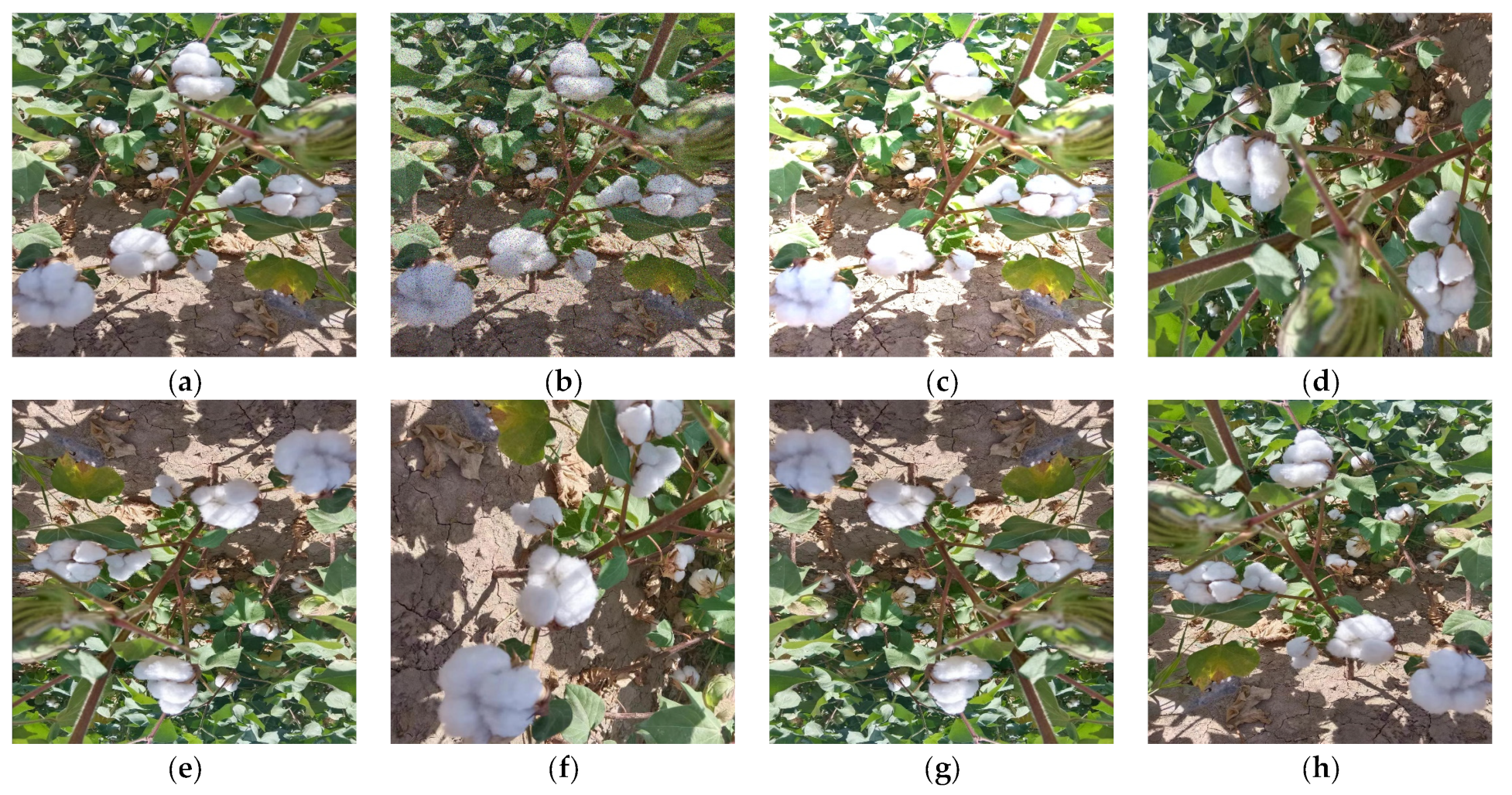
To avoid the model overfitting problem, data expansion is first achieved by using data enhancement methods such as adding noise, adjusting brightness, rotation, and flipping (Figure 2). Among them, adding noise can help the model better cope with complex environmental conditions, while rotating and flipping the image can improve the model’s ability to recognize target objects. In addition, luminance equalization can eliminate the effect of lighting changes in the environment on the detection performance. The above methods can double the amount of data and improve the robustness and recognition performance of the model. The original and enhanced images are used to create a dataset of 1500 images. The dataset is divided into training and test sets of 1200 and 300 images, respectively, according to the ratio of 8:2. To ensure that there are no enhanced images in the test set, only the original images are selected for the construction of the test set. Therefore, when labeling the data set, we numbered the original images and used them as the test data set to explain the performance of the model in cotton boll detection work. We used the graphical image annotation tool LabelImg “https://github.com/tzutalin/labelImg” (accessed on 5 October 2015) to manually draw regions of interest on all cotton boll images and generate XML files containing target type and coordinate information.

2.2.1. Mixup Data Enhancement

Mixup is an unconventional data enhancement method based on data correlation, which uses linear combinations to construct new training samples and labels [18]. The data labels are processed with the formulas shown as follows:
x ˜ = λ x i + 1 λ x j
y ˜ = λ y i + 1 λ y j
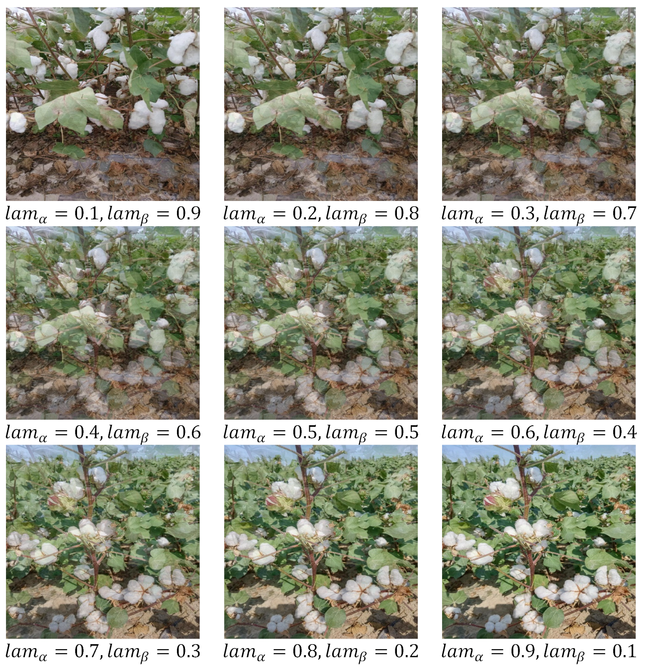
where x i , y i and x j , y j are training data (training samples and their corresponding labels) in the original dataset; λ is a parameter that obeys the β distribution; x ˜   is a mixture of training samples after the data augmentation operation; and y ˜ is the label of x ˜ . Figure 3 illustrates the data results after data augmentation with different fusion ratios.

2.2.2. Mosaic Data Enhancement

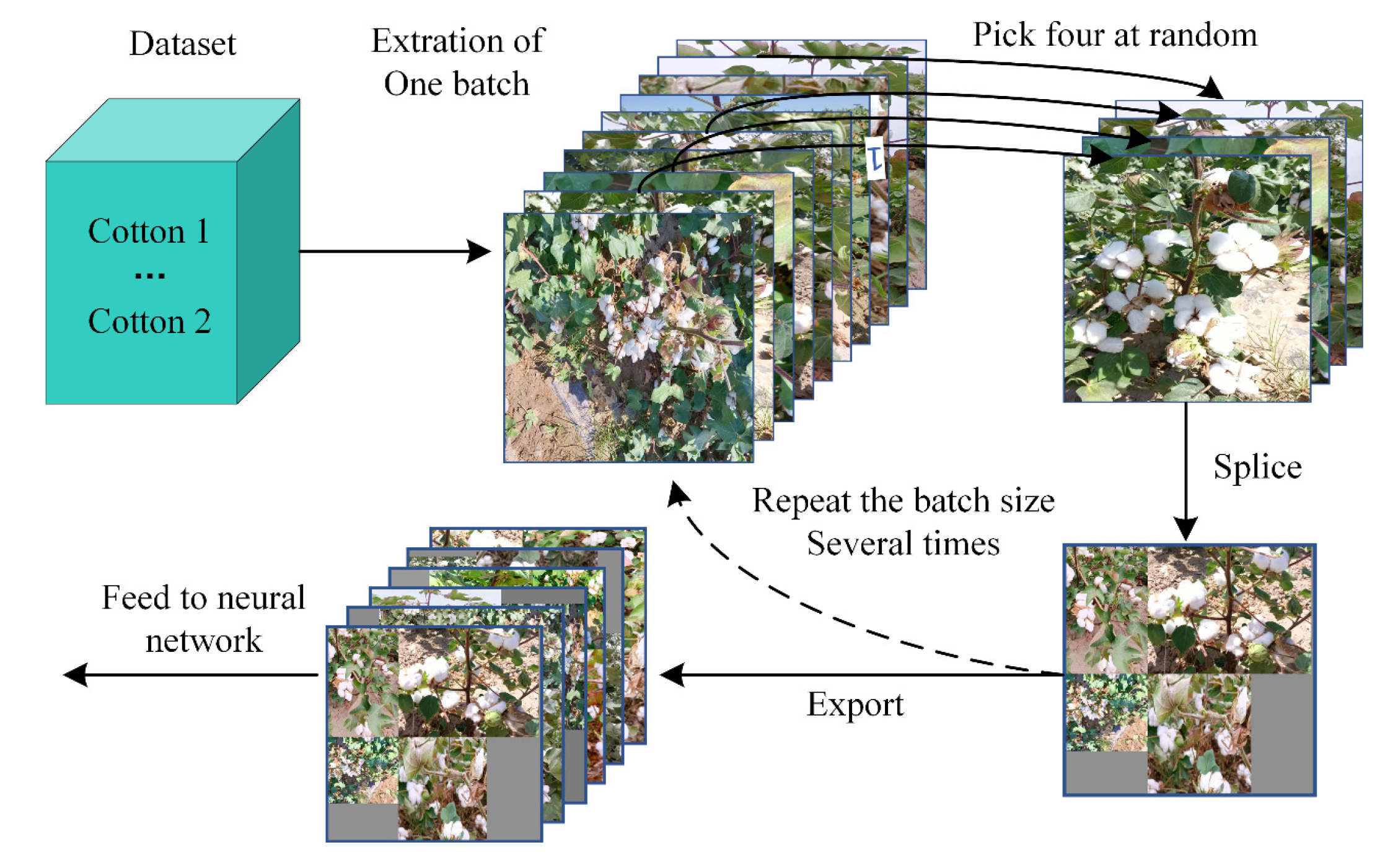
Mosaic data enhancement was first proposed for the YOLOv4 network, which is based on the principle of randomly cutting four images and combining them into one image as the newly generated training data, which greatly enriches the detection dataset, improves the robustness of the model, and reduces the GPU video memory usage Bochkovskiy et al. [19]. Figure 4 shows the workflow of mosaic data enhancement.

2.3. Experimental Environment

The improved model proposed in this study and all comparison models perform the cotton boll detection work on the GPU server. Table 1 shows the experimental configuration with a total of 1200 cotton boll images from different angles used for model training. The stochastic gradient descent (SGD) impulse value of the target detection algorithm used in this experiment is set to 0.937. The initial learning rate is set to 0.01, the weight decay is set to 0.0005, and the model is trained using a migration learning strategy.

2.4. Evaluation Indicators

To evaluate the performance of the algorithm, this study uses precision (P), recall (R), mean average precision (mAP), and F1 Score to assess the detection performance of the model. Precision is the probability of all predicted positive samples among the actual positive samples and is used to measure the prediction accuracy of positive sample results. Recall is the probability of actual positive samples being predicted as positive samples, which indicates the overall prediction accuracy. Both are calculated as follows:
Precision = T P T P + F P
Recall = T P T P + F N
Precision reflects the ability of the model to discriminate negative samples. The higher the precision, the better the model’s ability to discriminate negative samples. Recall reflects the model’s ability to identify positive samples. The higher the recall, the better the ability of the model to identify positive samples. F1 score is a combination of both. The higher the F1 score, the more stable the model.
F 1 = 2 Recall 1 + Precision 1 = 2 Precision Recall Precision + Recall
The average precision ( AP ) is the area value obtained by integrating the P-R curve composed of sample points with precision as the vertical coordinate and recall as the horizontal coordinate, and the larger the AP, the higher the accuracy of model recognition. Its calculation formula is as follows:
AP = 1 11 0 , 0.1 1.0 P s m o o t h i
The mean average precision (mAP) is the average value of AP. Typically, [email protected] and [email protected]:0.95 are used, where the former is the area of the curve at IoU = 0.5 and the latter is the average area of all P-R curves with IoU between 0.5 and 0.95. The calculation formula is as follows:
mAP = j = 1 s   A P j S
where S is the number of all categories, and the denominator is the sum of the APs of all categories. The target detection in this study was only one category of long-staple cotton, so AP = mAP.
In the model testing session, the mean absolute error (MAE), mean absolute percentage error (MAPE), coefficient of determination ( R 2 ), and root mean square error (RMSE) are used to evaluate the model. MAE reflects the average difference between the true number of cotton bolls and the number of detections, and the smaller the MAPE, the closer the model is to perfection. RMSE is a square root measure of the deviation between the observed and true values based on the mean square error (MSE), and it is often used as a measure of the performance of machine learning models. The formula is as follows:
MAE = 1 n 1 n m i c i
MAPE = 1 n 1 n m i c i m i × 100 %
R 2 = 1 1 n m i c i 2 1 n m i m ¯ i 2
RMSE = 1 n m i c i 2 n
where m i , c i , and m ¯ i denote the actual number of bolls, the predicted number of bolls, and the average actual number of bolls for the ith image, respectively. 𝑛 is the number of test images.

2.5. Improved Algorithm Construction

This section is divided into three parts, which introduce the YOLOv7 algorithm, the fusion of deformable convolution of backbone networks and the introduction of attention mechanism, and the optimization of loss function by WIoU based on dynamic non-monotonic focusing mechanism.

2.5.1. YOLOv7 Model Structure

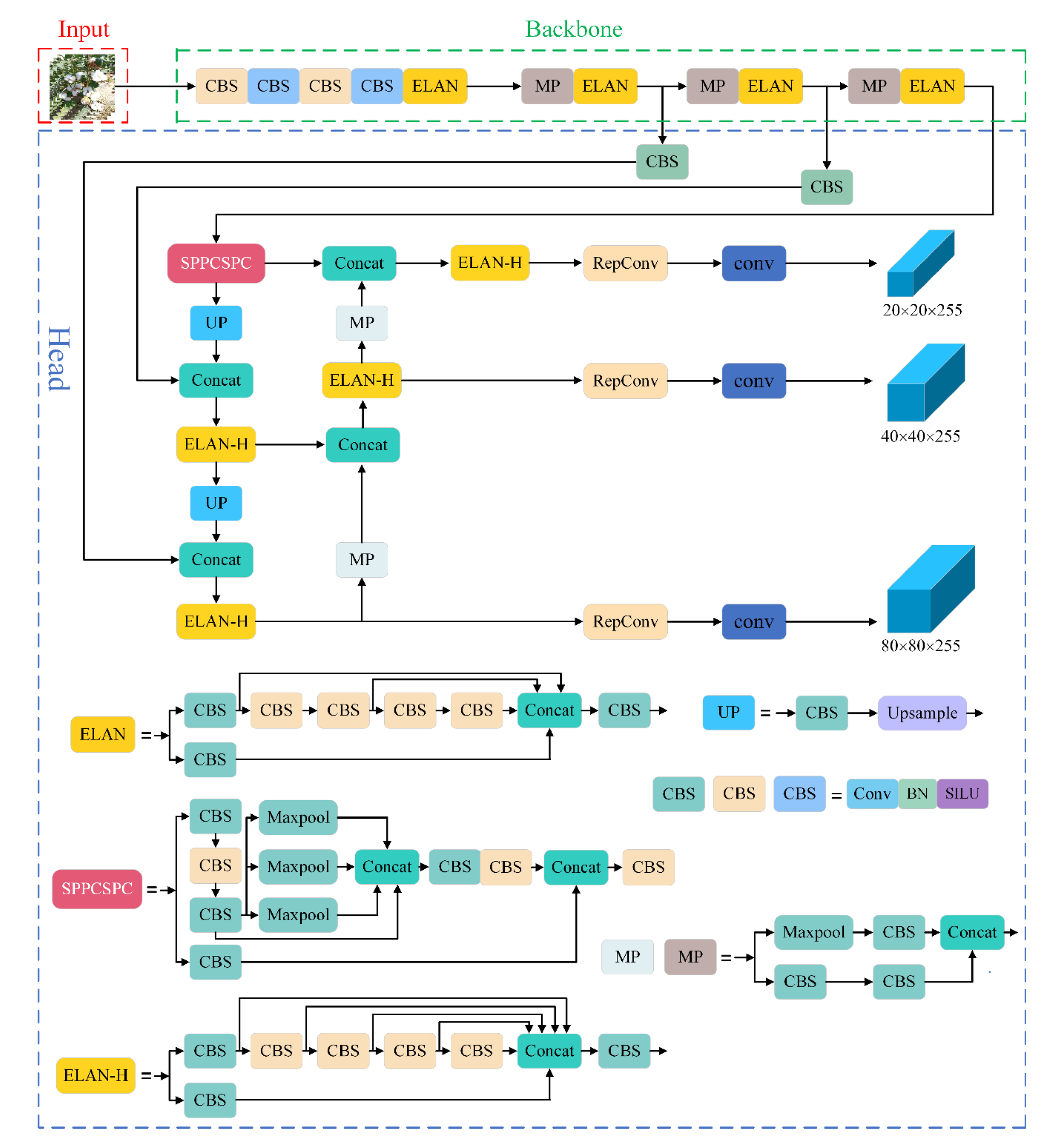
YOLOv7 is a single-stage state-of-the-art detection algorithm [20], which is based on the current classic target detection algorithm You Only Look Once (YOLO) [21], using YOLOv5 “https://github.com/ultralytics/yolov5” (accessed on 1 April 2020) as a starting point for improvement, and adding a multi-branch stacking module (E-ELAN) to the backbone of YOLOv7 compared to YOLOv5, and a transition module (MPConv) instead of the C3 module and normal convolution in YOLOv5. The use of expansion, shuffling, and merging of bases without destroying the original gradient path continuously improves the learning ability of the network. In the architecture of computational blocks, the channels and bases of computational blocks are expanded using group convolution to guide different groups of computational blocks to learn more diverse features. In addition, it designs some optimization modules and methods, called trainable “bags-of-freebies”, using reparameterizable convolution (RepConv) without constant connections in the architecture of heavy parametric convolution to provide more gradient diversity for different feature maps [22]. The model introduces an auxiliary detection head that uses soft labels generated by the optimization process to guide the learning of the head and the auxiliary head so that the generated soft labels can better represent the distribution and correlation between source data and objects and obtain more accurate results “https://github.com/RangiLyu/nanodet” (accessed on 29 March 2021). The model connects the batch normalization layer directly to the convolutional layer, allowing the integration of the normalized mean and variance of the batches into the deviations and weights of the convolutional layer during the inference phase. Finally, the exponential moving average (EMA) model is used as the final inference model to greatly improve the detection accuracy without increasing the inference cost [23], and the structure of the YOLOv7 network model is shown in Figure 5.

2.5.2. Model Improvements

(1)
Introducing deformable convolution
YOLOv7 uses deep convolutional networks for target feature extraction; in order to learn richer features, it needs to increase the depth of the network for feature learning, which increases not only the computational complexity but also the risk of overfitting. Meanwhile, convolutional networks have inherent drawbacks for modeling polymorphic targets due to the fact that convolutional networks only sample fixed positions of the input feature map [24]. In long-staple cotton boll detection, the receptive fields of all feature points in the same layer of the feature map in the convolutional network are the same, while different locations may correspond to different scales of the boll, so adaptive learning of the scale or receptive field size to localize the target is not possible.
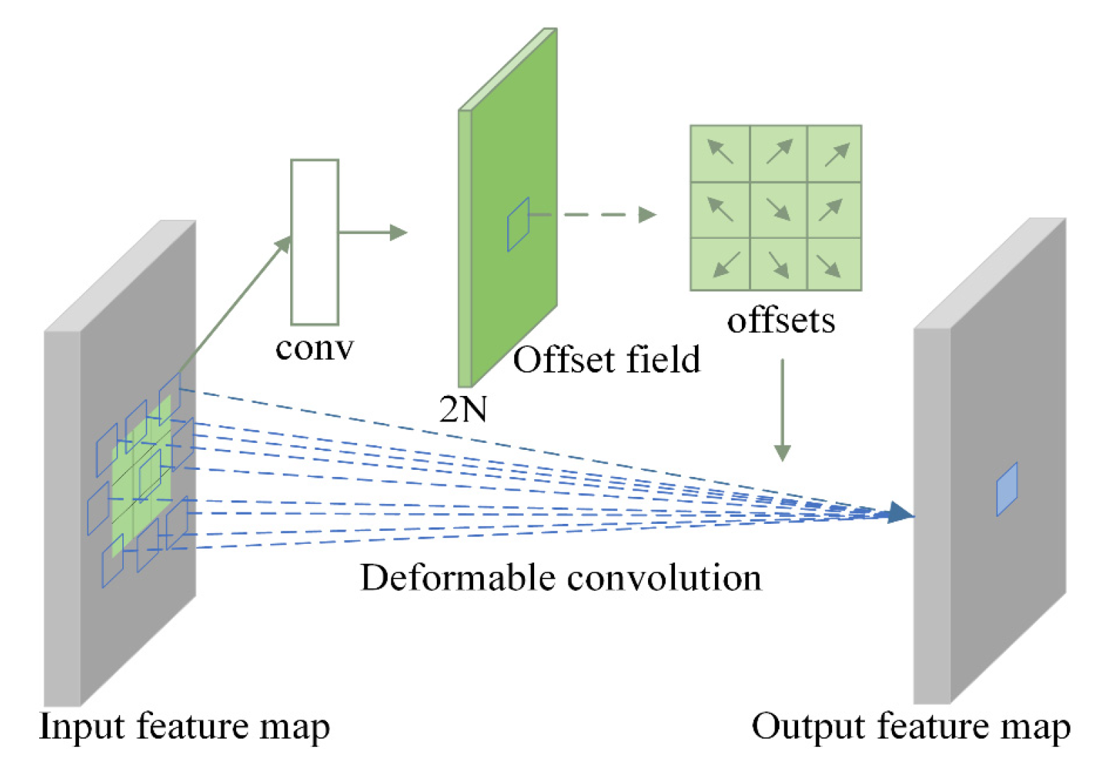
Deformable convolution can improve a model’s ability to model deformed targets. It uses parallel convolution layers to learn offsets that allow the convolution kernel to shift the sampling points on the input feature map to focus on regions or targets of interest [25]. Figure 6 shows the comparison between regular convolutional sample points and deformable convolutional sample points. Figure 7 shows the computational flow of deformable convolution, where the offset is calculated for the input feature map using the convolution layer, and the offset is used as the location of the sampling points. The number of channels of the output feature map is 3N (where N is the number of sample points of the convolution kernel), where 2N are the predicted offsets in the x- and y-directions, and the weights of the other N sample points must also be predicted since different sample points contribute differently to the features. In this way, the deformable convolution can flexibly adapt to the morphological changes of the target at different locations and scales, thus improving the detection accuracy of the model.
The conventional convolution operation is divided into two main steps: (1) sampling on the input feature map using a regular grid R; (2) weighting the sampled points using a convolution kernel w. R defines the size and dilation of the perceptual field, as shown in Equation (12), which defines a convolution kernel of size 3 × 3 and a dilation rate of 1.
R = 1 , 1 , 1 , 0 , , 0 , 1 , 1 , 1
For each position p 0 on the output feature map, the output value y p 0 is calculated as follows:
y p 0 = p n R w p n × x p 0 + p n  
In the deformable convolution operation, the expansion is performed by adding an offset Δ p n n = 1 , 2 , , N , N = R to the regular grid R while predicting a weight for each sample point. Then, the value of y p 0 for the same position p 0 becomes as shown as follows:
y p 0 = p n R w p n × x p 0 + p n + Δ p n × Δ m n
Since the offset Δ p n is usually fractional, the value of x must be calculated by bilinear interpolation as shown as follows:
x p = q   G q , p × x q
G q , p = g q x , p x × g q y , p y
g q , b = max 0 , 1 a b
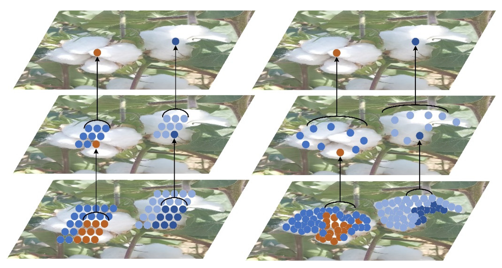
Figure 8 shows the comparison between the feature point perceptual fields of the regular and deformable convolution. The two feature points represent targets of different scales and shapes. With two layers of convolution operations, it can be seen that the feature points of the conventional convolution have a fixed-size perceptual field, while the perceptual sampling points of the deformable convolution can learn adaptively, which is more in line with the shape and size of the object itself and more conducive to feature extraction. Therefore, the deformable convolution can better adapt to the morphological changes of long-staple cotton and improve the modeling ability of the model for long-staple cotton with variable morphology, thus improving the accuracy and stability of long-staple cotton boll detection.
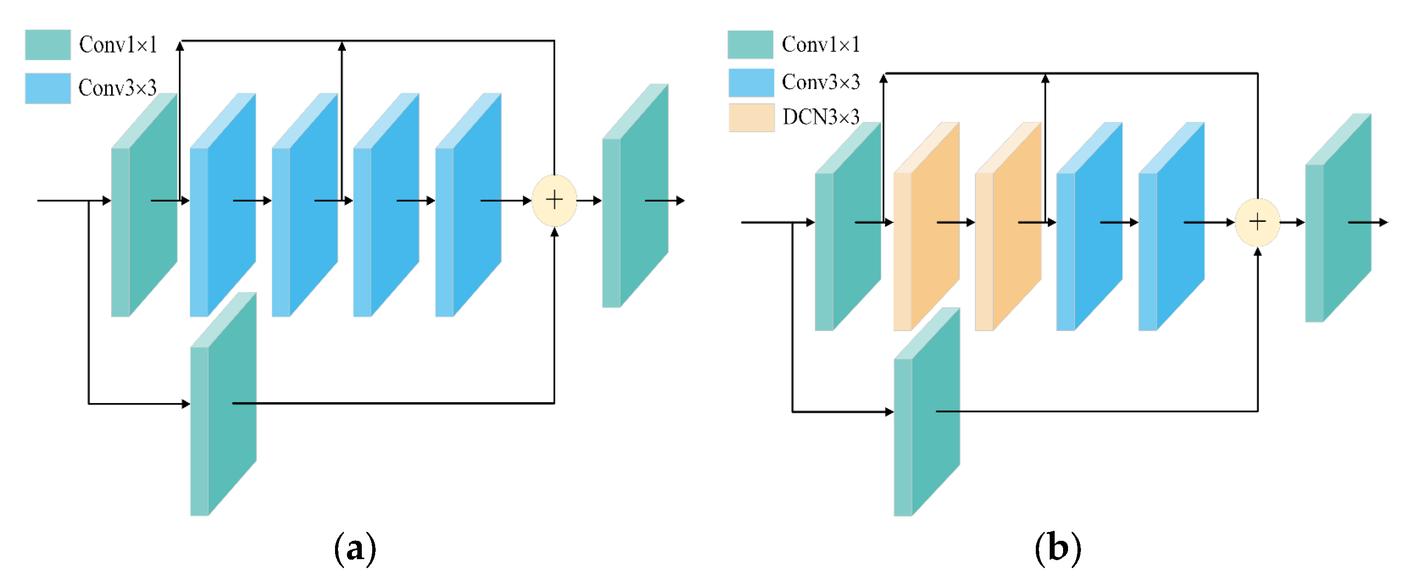
In the YOLOv7 backbone network, the feature extraction of the target is mainly performed by the ELAN multi-branch stacking module. As shown in Figure 9, the 3 × 3 convolution in the ELAN structure is used to perform feature extraction, and the 1 × 1 convolution is used to perform feature compression. For the deformable convolution, using the 1 × 1 deformable convolution to compute the offset for the sampling points may lead to sampling instability. Therefore, in this paper, part of the 3 × 3 convolution in the ELAN module is replaced by deformable convolution to improve the extraction of cotton boll features of different morphologies and scales by adding fewer computation resources. The introduction of deformable convolution can make the ELAN module more adaptable to the morphological changes of the target and improve the modeling ability of the model for deformed targets. Meanwhile, since deformable convolution can adaptively learn the position of sensory sampling points, it can better adapt to targets of different scales and shapes, thus improving the detection accuracy and robustness of the model.
(2)
YOLOv7 introduces SENet attention mechanism
The attention mechanism is a common data processing method that is widely used in machine learning tasks in various fields [26]. The core idea of the computer vision attention mechanism is to find the correlation between the original data and then highlight the important features, such as channel attention, pixel attention, multi-order attention, and so on. SENet is a typical implementation of the channel attention mechanism, and the module structure is shown in Figure 10.
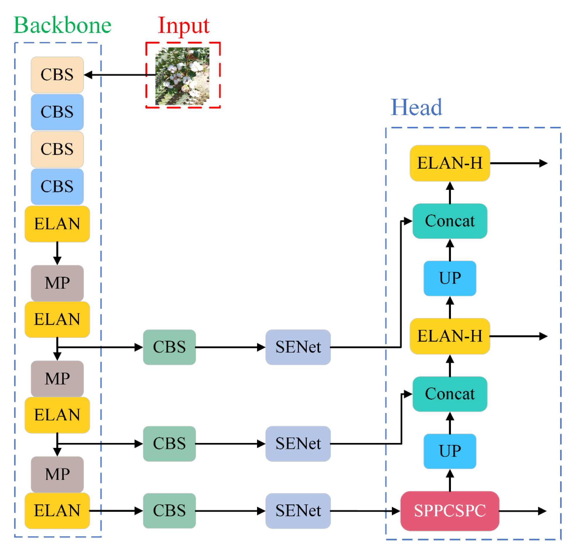
SENet can flexibly capture the connection between global and local information, allowing the model to obtain the object regions that require attention and assign greater weights to them, highlighting significantly useful features and suppressing the ignoring of irrelevant features, thus improving accuracy [27]. Convolutional block attention module (CBAM) adaptively adjusts the features by inferring the attention weights sequentially along both spatial and channel dimensions and then multiplying them with the original feature map to adjust, and its model is less complex and computationally intensive [28]. Coordinate attention (CA) performs global average pooling in two directions, height, and width, respectively, and then stitches the feature maps of these two directions together, which can effectively handle the relationship between channels [29]. In this paper, the SENet module, CBAM module, and CA module are added after the backbone, the network structure is shown in Figure 11, and the models after adding each module are compared with various evaluation metrics.
(3)
WIoU loss
Intersection over union (IoU) is a common evaluation metric in target detection [30]; it calculates the loss by evaluating the distance between the model’s prediction box B and the true box Bgt. Compared with the traditional cross-entropy loss function, it can better handle the problems of category imbalance and localization accuracy in target detection, thus improving the detection performance of the model, and the IoU loss is not affected by the bounding box scale. However, the value is zero if the two boxes B and B gt do not overlap, which can lead to no return in the gradient and inaccurate detectors.
IoU = B B gt B B gt
To solve the problem of gradient disappearance, Rezatofighi et al. proposed to solve this problem by introducing a closed-loop penalty term consisting of real and prediction frames and constructing a generalized intersection over union (GIoU) loss [31]. Most of the existing studies consider many geometric factors of the prediction frame and real frame off and construct a penalty term R i to solve the problem of gradient disappearance, and most of the bounding box losses are based on additive losses and follow the following paradigm:
L i = L IoU + R i
All of these methods assume that the examples in the training data are of high quality and work to strengthen the fitting ability of the bounding box loss. However, long-staple cotton data in real environments have large morphological and size differences due to their background occlusion, which can cause greater interference with the accuracy and consistency of data labeling, resulting in a dataset containing more low-quality examples, which may jeopardize the improvement of model detection performance if the regression of low-quality examples is persistently reinforced with bounding box. Zhang et al. proposed an efficient intersection over union (EIoU) loss and proposed a regression version of focal loss [32] to focus the regression process on high-quality anchor frames [33], but it does not fully exploit the potential of the non-monotonic focusing mechanism because its focusing mechanism is static. To address this problem, this study establishes a WIoU [34] loss function based on a dynamic nonmonotonic focusing mechanism by defining an outlier parameter to describe the quality of the anchor frame and introducing a nonmonotonic focusing coefficient to dynamically assign the optimal gradient gain to the anchor frame. Its equation is as follows:
L W I o U   = r R W I o U   L IoU , r = β δ α β δ , R W I o U   1 , e , L I o U   0 , 1
R W I o U = exp ( x x g t   ) 2 + ( y y g t   ) 2 ( W g 2 + H g 2 ) *
β = L I o U * L I o U 0 , +
where R W I o U is mainly used to amplify the normal quality anchor frame by L I o U , L I o U mainly reduces the high-quality anchor frame by R W I o U , and significantly reduces its focus on the centroid distance in case of good overlap between the anchor frame and the target frame. β denotes the outlier, which describes the quality of the anchor frame, and r denotes the non-monotonic focus factor, which is used to compute a gradient gain allocation strategy that fits the current situation. To prevent R W I o U from generating gradients that hinder convergence, W g , H g is separated from the computational graph. This effectively eliminates the factors that hinder convergence, so no new metrics, such as aspect ratio, are introduced.

3. Results

3.1. Ablation Experiments

In the training process of YOLOv7, we use different data augmentation methods for comparison, and after getting the optimal model by training different datasets, we test the model performance on the test set, and the results are shown in Table 2.
From Table 2, it can be seen that using the mixup and mosaic data enhancement strategies based on the original data set, the detection precision increases by 0.28 and 0.17 percentage points, respectively, and the model precision increase is the highest using the Mixed data enhancement strategy, with a detection precision of up to 93.82%, and its recall and [email protected] values decrease by 0.11 compared to the mosaic data enhancement strategy, 0.08 percentage points, but the model inference speed (FPS) is improved, as the dataset may have limitations, the diversity of the dataset can be increased by data augmentation, making the model more adaptable to different scenarios, thus improving its generalization ability. Based on comprehensive analysis considerations, hybrid data augmentation is adopted as the data augmentation strategy during model training.

3.2. Introducing Attentional Mechanisms to Compare Experimental Results

In this paper, we tried to add three attention mechanisms, SENet, CBAM, and CA, respectively, after the backbone and designed three sets of experiments to compare the performance and accuracy of the model after adding these three modules. Table 3 shows the results of the effects of adding different attention mechanisms to the model. By comparing the three attention mechanisms, it is found that the introduction of the SENet and CA modules improves the detection accuracy of the model while adding less computational complexity, while the addition of the CBAM module reduces the model accuracy.
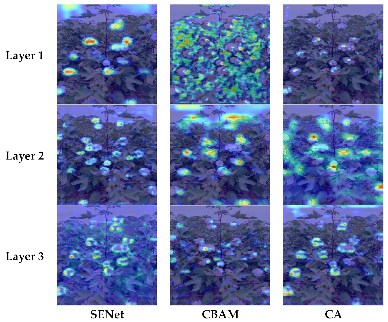
In addition, we used Grad-CAM to plot the heat map of the model after adding the attention module to visualize the focus of the network’s attention during seed detection. The results are shown in Figure 12. In the figure, the rows show the visualization of the different detection layers, and the columns show the results of the three detection layers after adding this module.
The qualitative analysis of the heat map images shows that CA has the worst detection performance for the first layer, which is used to detect small cotton bolls. On the contrary, CBAM considers the leaves of long-staple cotton plants as targets and avoids the targets being identified. The detection performance of SENet is the best, and the detection of some small targets by the other two algorithms is also affected by the background compared to the detection of medium targets, and SENet still performs well in the detection of medium objects. The CBAM algorithm still has some difficulties in the detection of large targets, while the performance of CA has improved but suffers from missed detections. From the quantitative analysis of the model evaluation results in Table 3, SENet has the highest accuracy, and CBAM has the worst performance. Based on the results of quantitative and qualitative analysis, we choose the SENet mechanism after the backbone network.

3.3. Impact of Improved Methods on the Model

Four sets of experiments were designed to compare the effects of all the improved methods on the model. The results of the improved models are shown in Table 4, where “√” indicates that the module is used in the model, and “×” indicates that the module is not used in the model.
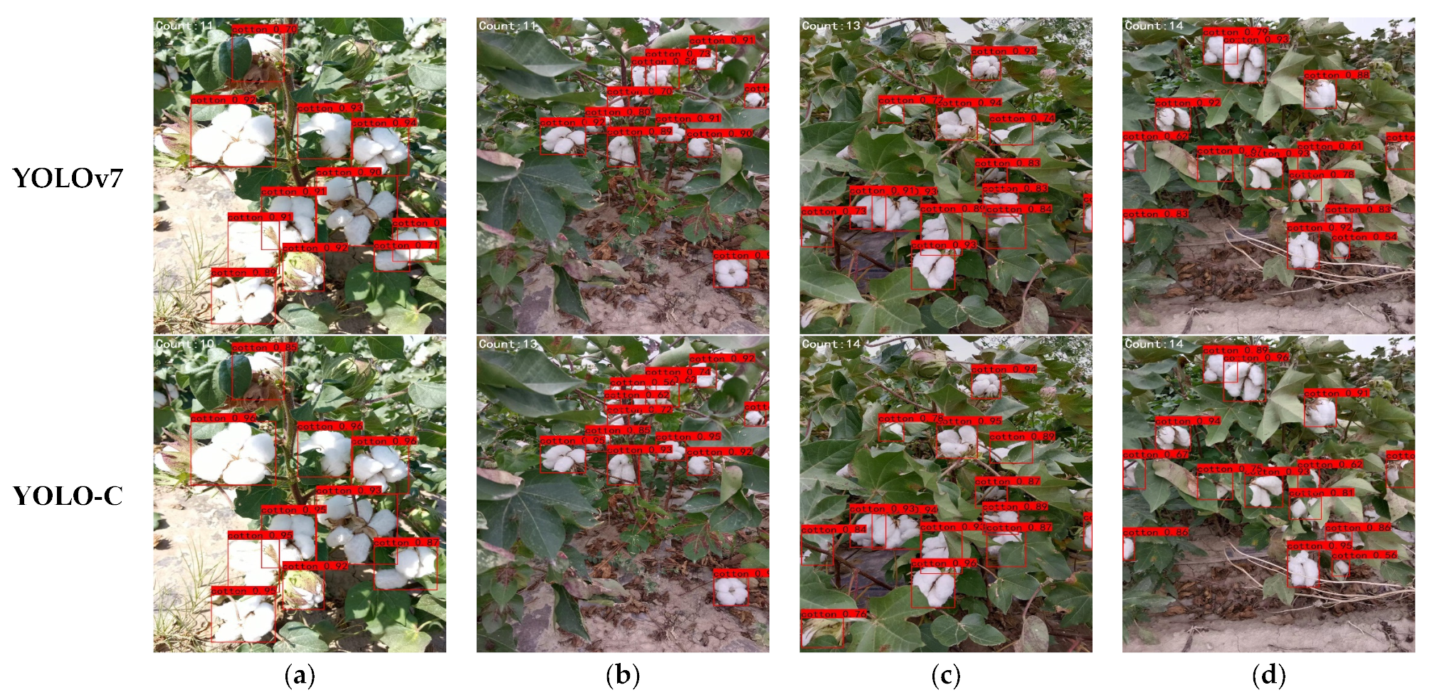
The analysis in Table 4 shows that replacing some of the 3 × 3 convolution operations in the ELAN module in the backbone with deformable convolution operations solves the problem that conventional convolution operations cannot perform adaptive learning of scale or receptive field size. Although feature extraction partially expands the receptive field, detection is still disturbed by the complex background and occlusion. Therefore, we introduce an attention mechanism that constructs correlations between raw data, highlights important features, improves the model’s detection performance in complex environments, reduces computation by removing redundant feature channels, and improves the model’s inference speed. Finally, we improve the loss function to reduce the competitiveness of high-quality anchor frames while reducing the harmful gradients generated by low-quality examples, focusing on normal-quality anchor frames and improving the overall performance of the detector. The detection results of the improved model in different environments are shown in Figure 13.

3.4. Comparison of the Improved Model with Other Models

To test the performance and accuracy of the algorithms proposed in this paper, our algorithms were compared with the current mainstream target detection algorithms, and each algorithm was evaluated and compared using P, R, and mAP evaluation metrics. The experimental results of the comparison are shown in Table 5.
As shown in Table 5, the performance of the improved model has a large improvement. As a two-stage algorithm, Faster R-CNN has good recognition accuracy. Unlike other one-stage algorithms, Faster R-CNN uses the region proposal network to generate potential regions, which are mapped to the feature map to obtain the feature matrix, so the model is more complex. In the single-stage algorithm, EfficientDet adopts EfficientNet as its convolutional network structure to improve the accuracy and efficiency of the model through techniques such as bidirectional feature pyramid network (BiFPN) and neural architecture search feature pyramid network (NAS-FPN) to improve the accuracy and efficiency of the model, but due to its multi-scale feature extraction and feature fusion techniques, it needs to process multiple scales of images during the training process, which increases the model complexity and time cost. RetinaNet adopts focal loss to solve the problem of category imbalance, which improves the model’s detection ability for small targets, but the weight of focal loss is not enough for the model. RetinaNet adopts Focal Loss to solve the problem of category imbalance, which improves the detection ability of the model for small targets, but its weight parameter needs to be adjusted by human experience, and a larger value may lead to unstable training and difficult convergence of the model. SSD and the YOLO family of algorithms, including YOLOv5, YOLOv7, and YOLOX, use multiple aspect ratios of anchor frames coupled with multiscale detection techniques to achieve faster runs than two-stage algorithms. YOLOX uses anchor-free frame techniques to achieve a good balance between speed and accuracy but has lower accuracy compared to YOLOv7.
Experimental results show that YOLO-C outperforms other detection algorithms in terms of precision, recall, and mAP. Compared with Faster R-CNN two-stage target detection, YOLO-C achieves higher average accuracy and stability performance. Compared to the single-stage target detection models EfficientDet and RetinaNet, the models show a significant improvement in accuracy and inference speed. Compared to the YOLO series of algorithms, the [email protected] of the model improved by 6.35% and 6.03% over YOLOv5 and YOLOX, respectively, and the [email protected] improved from 95.59% to 97.19% over the original YOLOv7, and it improves the accuracy and recall as well as the speed of model inference.
Figure 14 shows the detection performance of YOLOv7 and the improved model for the same data, as shown in Figure 14a; the fused variable convolution of the backbone part gives the improved model the ability to learn adaptively for scale and perceptual field, which effectively reduces the model’s false detection rate, as shown in Figure 14b,c; the introduction of the SENet attention mechanism enables the model to detect missed detections even in complex background cotton bolls. The improved model occasionally identifies targets with low confidence, as shown in Figure 14d, due to larger foliage obscuring the boll fraction and fewer boll pixel points.

3.5. Evaluation of Experimental Results of Cotton Boll Testing

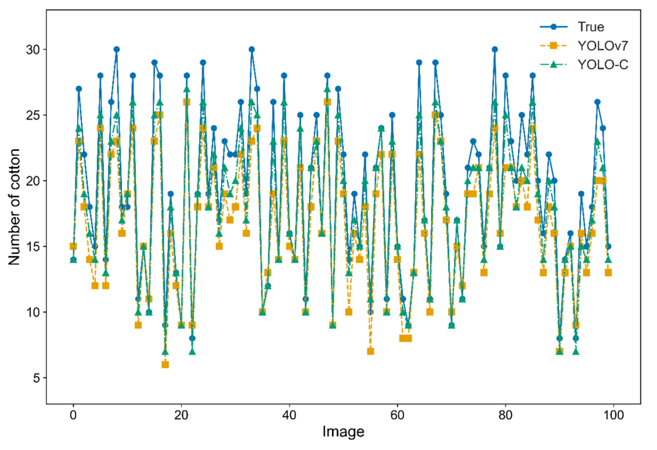
We randomly selected 100 images in the test set and used YOLOv7 and YOLO-C for cotton boll detection and compared the detection results with the real data to evaluate the performance of the model. Figure 15 shows the detection results of the model, and the improved model achieves good results in boll detection with different numbers of populations. Table 6 shows the detection performance of YOLOv7 and YOLO-C models.
The coefficient of determination R 2   of YOLOv7 in cotton boll detection was 0.90, while the YOLO-C model reached 0.96. Compared with the original model, the RMSE and MAE values of YOLO-C were reduced by 41.3% and 46.4%, respectively, indicating that YOLO-C effectively improves the performance of boll detection and has practical applications in cotton field management.

4. Discussion

Long-staple cotton is an important economic, strategic crop; due to the planting area restrictions, coupled with its high management level requirements, there are few studies on automated long-staple cotton boll detection and counting that have been reported. Most of the existing long-staple cotton boll detection and counting are manual; manual detection is inefficient, and the complex field environment can increase the difficulty of the observer’s work. Therefore, this study proposes an improved deep learning algorithm YOLO-C for automatic cotton boll detection and counting with an algorithm accuracy of 95.75%, which is 1.93% higher in accuracy, 1.01% higher in recall, and 1.6% higher in [email protected] than the YOLOv7 algorithm before improvement and one hundred images were randomly selected for testing YOLO-C with mean square error and coefficient of determination ( R 2 ) were 1.88 and 0.96, respectively. This method can provide an effective means to achieve precise agricultural control. In addition, there are few boll detection counting methods for long-staple cotton, a crop with large morphological and size differences, and this study fills this gap to some extent.
Based on the YOLOv7 model, this study improves the model by considering both the complex environmental factors of field crops and their characteristics in the detection process so that the model has a higher target detection capability, improves the robustness of the model, and is more adaptable to realistic scenarios. Compared with other boll detection techniques, the proposed boll detection method can achieve efficient boll detection and counting in complex field environments. Most of the existing boll detection methods are based on image segmentation, and the method based on image segmentation to detect and count cotton boll can be adapted to different scenes and environments by selecting different segmentation algorithms and parameters, which has a certain flexibility and adaptability [5], but its anti-interference ability is poor, which can lead to missed detection or false detection and affect the accuracy and robustness of counting, and the method is sensitive to complex field environments and occlusion. The machine learning-based cotton boll detection method can learn more accurate features and improve the detection ability of the model by manually designing features on the data [9], but there are more influencing factors for cotton boll detection in real environments, and the manual design and selection of features is a huge workload, the correlation between the selected features and the target recognition cannot be guaranteed, and the adaptability and generalization ability of the model is poor. Different data sources also have a great impact on cotton boll detection. Cotton boll detection based on remote sensing images can quickly obtain the number of cotton bolls in a large area of cotton fields [6], but it can only detect the canopy boll, and it is difficult to effectively detect the middle and bottom bolls because the bolls are severely obscured by aerial images under a vertical structure.
There are several limitations to this study. First, the environments studied in this paper did not take into account disturbances caused by the external environment, such as birds in a large field environment, and the data set was collected without considering disturbances caused by severe weather, which may not be representative enough. In the future, we will collect more long-staple cotton data sets under more conditions. Second, there are missed detections in the dense cotton boll image detection results. In the post-processing process of target detection, non-maximum suppression (NMS) is used to eliminate redundant prediction frames on the same object, which mainly achieves the final result by setting the scores of neighboring detection frames that overlap with the highest-scoring detection frame to zero. For two objects with a large degree of overlap, NMS [35] tends to treat the real frame of one of the objects as redundant and eliminate it in the process, which leads to poor performance of the model in the dense seed detection process. To solve this problem, in the future, we consider using the SoftNMS method [36], which uses a weighting function to attenuate the fraction of prediction frames with a large degree of overlap, to improve the detection performance of dense cotton boll detection. The objective of this study is to explore different deep neural network models to determine the effectiveness of the best model for cotton boll detection in a wide range of field environments and the applicability of the model deployment on hardware to improve precision agriculture control.

5. Conclusions

In this study, a large-scale long-staple cotton dataset including 1500 long-staple cotton images is constructed to provide data support for long-staple cotton yield monitoring visualization research; an improved YOLOv7 algorithm YOLO-C incorporating deformable convolution and SENet modules is proposed, and a loss function based on the dynamic non-monotonic focusing mechanism is established to improve the original loss function. Tested on long-staple cotton images in different environments, the improved model improves accuracy, recall, and mAP and shows better performance in the detection counting session; it extends the applicability of YOLO-C to models in complex environments and improves the robustness of the model. The model achieved better detection results in the long-staple cotton boll detection task in a complex environment. The method has some reference value for yield prediction and intelligent field management in the cotton picking season.
Future research will continue to optimize the network structure of the proposed algorithm and deploy the network in the hardware environment used in field farming. Our goal is to construct a long-staple cotton growth class based on accurate long-staple cotton boll detection by analyzing individual cotton boll fruits for more accurate long-staple cotton yield prediction. This provides a reliable and effective solution for achieving precision agriculture.

Author Contributions

Conceptualization, Z.L. and X.L.; methodology, Z.L.; software, Z.L. and G.C.; validation, Z.L., G.C. and M.X.; formal analysis, Z.L.; resources, X.L.; writing—original draft preparation, Z.L.; writing—review and editing, Z.L., X.L. and X.J.; visualization, T.L.; supervision, X.L.; funding acquisition, X.L. All authors have read and agreed to the published version of the manuscript.

Funding

This research was funded by the National Natural Science Foundation of China under the project “Research on Bionic Vision and Adaptive Grasping Method of Xinjiang Long-staple Cotton Picking Robot” 52265003, in part by the Xinjiang Uygur Autonomous Region under the project “Research on Human-like Picking Robot 20227SYCCX0061, and partly supported by the “Research on Automatic and Intelligent Machinery and Equipment for Vegetables around Tarim Basin” 2022A02005-5, a major project of Xinjiang Uygur Autonomous Region. Supported by the central government-led local project “Research and Base Construction of Facility Green Fruit and Vegetable Production and Processing Engineering and Intelligent Equipment in Xinjiang” ZYYD2023B01.

Data Availability Statement

Not applicable.

Acknowledgments

We sincerely thank Xiuliang Jin of the Institute of Crop Science, Chinese Academy of Agricultural Sciences, for his guidance and Tao Lin of the Institute of Cash Crops, Xinjiang Academy of Agricultural Sciences, for his help.

Conflicts of Interest

The authors declare no conflict of interest.

References

  1. Felgueiras, C.; Azoia, N.G.; Goncalves, C.; Gama, M.; Dourado, F. Trends on the cellulose-based textiles: Raw materials and technologies. Front. Bioeng. Biotechnol. 2021, 9, 608826. [Google Scholar] [CrossRef] [PubMed]
  2. Auernhammer, H. Precision farming—The environmental challenge. Comput. Electron. Agric. 2001, 30, 31–43. [Google Scholar] [CrossRef]
  3. Saleem, M.H.; Potgieter, J.; Arif, K.M. Automation in agriculture by machine and deep learning techniques: A review of recent developments. Precis. Agric. 2021, 22, 2053–2091. [Google Scholar] [CrossRef]
  4. Liu, J.; Lai, H.; Jia, Z. Image segmentation of cotton based on ycbccr color space and fisher discrimination analysis. Acta Agron. Sin. 2011, 37, 1274–1279. [Google Scholar]
  5. Sun, S.; Li, C.; Paterson, A.H.; Chee, P.W.; Robertson, J.S. Image processing algorithms for infield single cotton boll counting and yield prediction. Comput. Electron. Agric. 2019, 166, 104976. [Google Scholar] [CrossRef]
  6. Yeom, J.; Jung, J.; Chang, A.; Maeda, M.; Landivar, J. Automated open cotton boll detection for yield estimation using unmanned aircraft vehicle (uav) data. Remote Sens. 2018, 10, 1895. [Google Scholar] [CrossRef] [Green Version]
  7. Bawa, A.; Samanta, S.; Himanshu, S.K.; Singh, J.; Kim, J.; Zhang, T.; Chang, A.; Jung, J.; Delaune, P.; Bordovsky, J.; et al. A support vector machine and image processing based approach for counting open cotton bolls and estimating lint yield from uav imagery. Smart Agric. Technol. 2023, 3, 100140. [Google Scholar] [CrossRef]
  8. Li, Y.; Cao, Z.; Lu, H.; Xiao, Y.; Zhu, Y.; Cremers, A.B. In-field cotton detection via region-based semantic image segmentation. Comput. Electron. Agric. 2016, 127, 475–486. [Google Scholar] [CrossRef]
  9. Rodriguez-Sanchez, J.; Li, C.; Paterson, A.H. Cotton yield estimation from aerial imagery using machine learning approaches. Front. Plant Sci. 2022, 13, 870181. [Google Scholar] [CrossRef] [PubMed]
  10. Zeng, T.; Li, S.; Song, Q.; Zhong, F.; Wei, X. Lightweight tomato real-time detection method based on improved yolo and mobile deployment. Comput. Electron. Agric. 2023, 205, 107625. [Google Scholar] [CrossRef]
  11. Wang, D.; He, D. Channel pruned yolo v5s-based deep learning approach for rapid and accurate apple fruitlet detection before fruit thinning. Biosyst. Eng. 2021, 210, 271–281. [Google Scholar] [CrossRef]
  12. Sozzi, M.; Cantalamessa, S.; Cogato, A.; Kayad, A.; Marinello, F. Automatic bunch detection in white grape varieties using yolov3, yolov4, and yolov5 deep learning algorithms. Agronomy 2022, 12, 319. [Google Scholar] [CrossRef]
  13. Cardellicchio, A.; Solimani, F.; Dimauro, G.; Petrozza, A.; Summerer, S.; Cellini, F.; Renò, V. Detection of tomato plant phenotyping traits using yolov5-based single stage detectors. Comput. Electron. Agric. 2023, 207, 107757. [Google Scholar] [CrossRef]
  14. Xu, R.; Li, C.; Paterson, A.H.; Jiang, Y.; Sun, S.; Robertson, J.S. Aerial images and convolutional neural network for cotton bloom detection. Front. Plant Sci. 2018, 8, 2235. [Google Scholar] [CrossRef] [Green Version]
  15. Singh, N.; Tewari, V.K.; Biswas, P.K.; Dhruw, L.K. Lightweight convolutional neural network models for semantic segmentation of in-field cotton bolls. Artif. Intell. Agric. 2023, 8, 1–19. [Google Scholar] [CrossRef]
  16. Fue, K.G.; Porter, W.M.; Rains, G.C. Deep Learning Based Real-Time Gpu-Accelerated Tracking and Counting of Cotton Bolls under Field Conditions Using a Moving Camera; American Society of Agricultural and Biological Engineers: St. Joseph, MI, USA, 2018; p. 1. [Google Scholar]
  17. Tedesco-Oliveira, D.; Da Silva, R.P.; Maldonado, W., Jr.; Zerbato, C. Convolutional neural networks in predicting cotton yield from images of commercial fields. Comput. Electron. Agric. 2020, 171, 105307. [Google Scholar] [CrossRef]
  18. Zhang, H.; Cisse, M.; Dauphin, Y.N.; Lopez-Paz, D. Mixup: Beyond empirical risk minimization. arXiv 2017, arXiv:1710.09412. [Google Scholar]
  19. Bochkovskiy, A.; Wang, C.; Liao, H.M. Yolov4: Optimal speed and accuracy of object detection. arXiv 2020, arXiv:2004.10934. [Google Scholar]
  20. Wang, C.; Bochkovskiy, A.; Liao, H.M. Yolov7: Trainable bag-of-freebies sets new state-of-the-art for real-time object detectors. arXiv 2022, arXiv:2207.02696. [Google Scholar]
  21. Redmon, J.; Divvala, S.; Girshick, R.; Farhadi, A. You Only Look Once: Unified, Real-Time Object Detection; Cornell University Library: Ithaca, NY, USA, 2016; pp. 779–788. [Google Scholar]
  22. Ding, X.; Zhang, X.; Ma, N.; Han, J.; Ding, G.; Sun, J. Repvgg: Making vgg-style convnets great again, Proceedings of the IEEE/CVF conference on computer vision and pattern recognition. arXiv 2021, arXiv:2101.03697. [Google Scholar]
  23. Tarvainen, A.; Valpola, H. Mean teachers are better role models: Weight-averaged consistency targets improve semi-supervised deep learning results. Adv. Neural Inf. Process. Syst. 2017, 30, 1195–1204. [Google Scholar]
  24. Yusuf, A.A.; Chong, F.; Xianling, M. An analysis of graph convolutional networks and recent datasets for visual question answering. Artif. Intell. Rev. 2022, 55, 6277–6300. [Google Scholar] [CrossRef]
  25. Wang, W.; Dai, J.; Chen, Z.; Huang, Z.; Li, Z.; Zhu, X.; Hu, X.; Lu, T.; Lu, L.; Li, H.; et al. Internimage: Exploring large-scale vision foundation models with deformable convolutions. arXiv 2022, arXiv:2211.05778. [Google Scholar]
  26. Guo, M.; Xu, T.; Liu, J.; Liu, Z.; Jiang, P.; Mu, T.; Zhang, S.; Martin, R.R.; Cheng, M.; Hu, S. Attention mechanisms in computer vision: A survey. Comput. Vis. Media 2022, 8, 331–368. [Google Scholar] [CrossRef]
  27. Hu, J.; Shen, L.; Albanie, S.; Sun, G.; Wu, E. Squeeze-and-excitation networks. arXiv 2019, arXiv:1709.01507. [Google Scholar]
  28. Woo, S.; Park, J.; Lee, J.; Kweon, I.S. Cbam: Convolutional block attention module. arXiv 2018, arXiv:1807.06521. [Google Scholar]
  29. Hou, Q.; Zhou, D.; Feng, J. Coordinate attention for efficient mobile network design. arXiv 2021, arXiv:2103.02907. [Google Scholar]
  30. Yu, J.; Jiang, Y.; Wang, Z.; Cao, Z.; Huang, T. Unitbox: An Advanced Object Detection Network; Cornell University Library, arXiv.org: Ithaca, NY, USA, 2016; pp. 516–520. [Google Scholar]
  31. Rezatofighi, H.; Tsoi, N.; Gwak, J.; Sadeghian, A.; Reid, I.; Savarese, S. Generalized intersection over union: A metric and a loss for bounding box regression. In Proceedings of the IEEE/CVF Conference on Computer Vision and Pattern Recognition, California, CA, USA, 15–18 October 2019. [Google Scholar]
  32. Lin, T.; Goyal, P.; Girshick, R.; He, K.; Dollár, P. Focal loss for dense object detection. arXiv 2018, arXiv:1708.02002. [Google Scholar]
  33. Zhang, Y.; Ren, W.; Zhang, Z.; Jia, Z.; Wang, L.; Tan, T. Focal and efficient iou loss for accurate bounding box regression. Neurocomputing 2022, 506, 146–157. [Google Scholar] [CrossRef]
  34. Tong, Z.; Chen, Y.; Xu, Z.; Yu, R. Wise-iou: Bounding box regression loss with dynamic focusing mechanism. arXiv 2023, arXiv:2301.10051. [Google Scholar]
  35. Neubeck, A.; Van Gool, L. Efficient non-maximum suppression. In Proceedings of the 18th International Conference on Pattern Recognition (ICPR’06), Hong Kong, China, 20–24 August 2006; pp. 850–855. [Google Scholar]
  36. Bodla, N.; Singh, B.; Chellappa, R.; Davis, L.S. Soft-nms—Improving object detection with one line of code. arXiv 2017, arXiv:1704.04503. [Google Scholar]
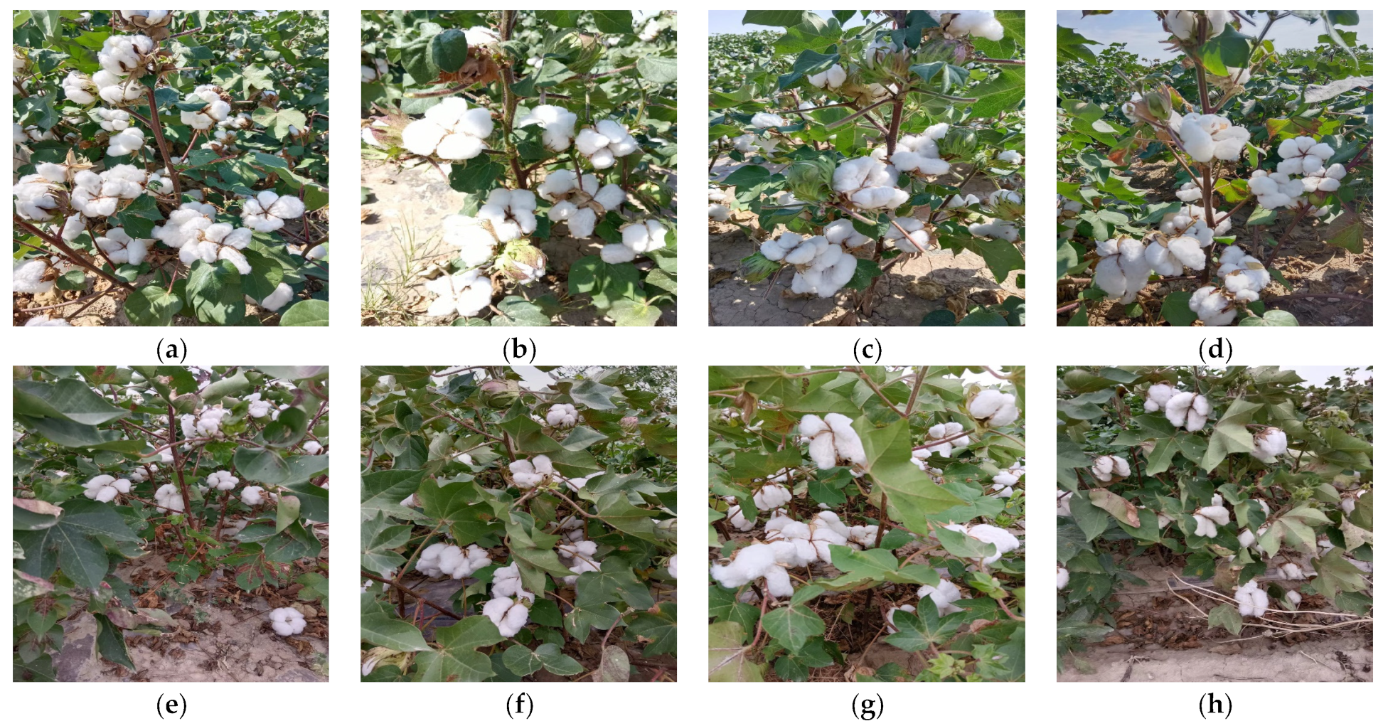
Figure 1. Examples of cotton peach images at different times: (a) 10:00 to 12:00 (sunny), (b) 12:00 to 14:00 (sunny), (c) 14:00 to 16:00 (sunny), (d) 16:00 to 18:00 (sunny), (e) 18:00 to 20:00 (sunny), (f) 10:00 to 12:00 (cloudy), (g) 14:00 to 16:00 (cloudy), (h) 18:00 to 20:00 (cloudy).
Agronomy 13 01988 g001
Figure 2. Data enhancement: (a) original image, (b) noise, (c) adjusted brightness, (d) rotated by 90°, (e) rotated by 180°, (f) rotated by 270°, (g) flipped vertically, (h) flipped horizontally.
Agronomy 13 01988 g002
Figure 3. Results of cotton boll data enhanced by mixup data with different fusion ratios, where l a m α and l a m β are the fusion ratios of the images and l a m α + l a m β = 1 .
Agronomy 13 01988 g003
Figure 4. Mosaic data enhancement process.
Agronomy 13 01988 g004
Figure 5. YOLOv7 network structure diagram.
Agronomy 13 01988 g005
Figure 6. Comparison of sampling points between conventional 3 × 3 convolution and deformable convolution.
Agronomy 13 01988 g006
Figure 7. Deformable convolution computational flow.
Agronomy 13 01988 g007
Figure 8. Comparison of feature point perceptual fields for regular and deformable convolution.
Agronomy 13 01988 g008
Figure 9. (a) shows the ELAN network structure, and (b) shows the ELAN after fusing deformable convolution.
Agronomy 13 01988 g009
Figure 10. SENet attention mechanism network structure.
Agronomy 13 01988 g010
Figure 11. Adding the SENet mechanism to the network.
Agronomy 13 01988 g011
Figure 12. Heat map of the model with different attention mechanisms.
Agronomy 13 01988 g012
Figure 13. Detection effect of the model under different environments: (a) highlight, (b) block, (c) Mulch, (d) dense.
Agronomy 13 01988 g013
Figure 14. Comparison of the effect before and after model improvement. (a) 12:00 to 14:00 (sunny), (b) 18:00 to 20:00 (sunny), (c) 10:00 to 12:00 (cloudy), (d) 18:00 to 20:00 (cloudy).
Agronomy 13 01988 g014
Figure 15. Experimental results of YOLOv7 and YOLO-C model detection.
Agronomy 13 01988 g015
Table 1. Experimental configuration.
ConfigurationParameter
CPUIntel (R) Xeon (R) Platinum 8350C
GPUNVIDIA GeForce RTX3090
Operating systemWindows 10
Accelerated environmentCUDA 11.1
Development environmentPycharm 2021
LibrariesPyTorch 1.11.0 Python 3.8
Table 2. Model training effects under different training techniques.
MosaicMixupPRF1[email protected][email protected]:0.95FPS
××93.30%91.64%0.9295.66%63.12%44
×93.47%91.75%0.9395.67%63.51%45
×93.58%91.64%0.9395.30%62.45%45
93.82%91.64%0.9395.59%63.52%48
Table 3. Results of adding the attention mechanism to the model.
CBAMSECAPRF1[email protected][email protected]:0.95FLOPS (G)
×××93.82%91.64%0.9395.59%63.52%105.47
××93.38%91.53%0.9295.50%63.12%105.49
××94.86%92.57%0.9396.74%64.12%105.49
××93.57%91.75%0.9395.43%63.22%105.49
Table 4. Comparison of improved models.
DCNSENetWIoUPRF1[email protected][email protected]:0.95FPS
×××93.82%91.64%0.9395.59%63.52%48
××94.34%91.53%0.9495.17%63.10%46
×95.25%92.44%0.9496.90%64.17%48
95.75%92.65%0.9497.19%64.31%49
Table 5. Comparison of improved network and mainstream target detection model.
MethodsPR[email protected][email protected]:0.95FPS
Faster R-CNN85.74%86.12%89.43%58.68%13
SSD78.18%76.40%80.05%50.40%26
EfficientDet85.68%89.98%92.93%59.80%24
RetinaNet86.02%87.17%91.06%56.35%19
YOLOv590.28%85.08%90.84%59.19%49
YOLOv793.82%91.64%95.59%63.52%48
YOLOX89.52%84.92%91.16%59.67%51
YOLO-C95.75%92.65%97.19%64.31%49
Table 6. RMSE, MAE, MAPE, and R 2 of YOLOv7 and YOLO-C models for cotton boll detection.
ModelRMSEMAEMAPE R 2
YOLOv73.202.6512.02%0.90
YOLO-C1.881.426.72%0.96
Disclaimer/Publisher’s Note: The statements, opinions and data contained in all publications are solely those of the individual author(s) and contributor(s) and not of MDPI and/or the editor(s). MDPI and/or the editor(s) disclaim responsibility for any injury to people or property resulting from any ideas, methods, instructions or products referred to in the content.