1. Introduction
Pepper fruits are a source of natural pigments and antioxidants, including vitamin C, flavonoids, and phenolic acids, as well as carotenoids [
1]. Given the nutraceutical and anticancer properties of pepper compounds, they are important preventive factors against many diseases, e.g., cardiovascular disease, type II diabetes, and other aging-associated disorders [
2,
3,
4]. Pepper cultivation is economically valuable, nutritionally beneficial, and supports job creation and rural livelihoods. It contributes to crop diversification, genetic diversity, and international trade, playing a significant role in global agriculture.
Understanding the pattern of length and growth of pepper (Capsicum annum L.) fruits is crucial for effective cultivation planning, yield estimation, quality assessment, pest management, and scientific research. It allows farmers to schedule planting, fertilization, and harvesting activities, estimate yields, assess fruit quality, detect pest or disease issues, and develop improved varieties. By tracking fruit growth, growers can optimize their practices, enhance productivity, and ensure successful pepper cultivation.
According to Rêgo et al. [
5], fruit weight, length, and diameter are essential in many horticultural crops, including pepper plants. In this context, evaluating the behavior of these characteristics throughout the crop cycle is fundamental for the researcher when deciding to develop appropriate management techniques and harvest fruits at appropriate growth stages [
6].
In many cases, it is desirable to quantify the growth of horticultural products with functions [
7]. Usually, the development of living beings shows a distinct behavior, starting slowly, passing to an exponential phase, and tending to stabilize at the end. This fact makes the method of nonlinear models an excellent alternative to adjust such growth behaviors. For pepper data, we can cite some research examples that used NLM to fit growth curves, such as [
6,
7,
8].
Usually, in its applications, the estimation method is done traditionally, whereby the growth characteristics are obtained through an adjustment per individual. In this case, information about all individuals must be evaluated at a second stage, regardless whether they belong to the same group. An alternative capable of solving this problem and still allowing the inclusion of individual and group effects in the same model is Nonlinear Mixed-Effect Models (NLME).
This method has some advantages over traditional (non-mixed) models. Among them, we can mention the allowing the individual modeling of accessions/individuals as random effects, together with the inclusion of the fixed effects of species, environment, management, or another source of variation. Lindstrom and Bates [
9] claim that the notion that individuals’ responses all follow a similar functional form with varying parameters among individuals seems to be appropriate in many situations.
Several researchers have used NLME modeling in different contexts, including the development of animal growth curves, as can be seen in Alves et al. [
10] for Guzerá cattle and in Araujo Neto et al. [
11] for dairy buffaloes. In addition to applications in the animal field, this methodology has been recurrently applied in the silvicultural area, such as in the development of height-diameter models [
12,
13,
14,
15,
16], crown-base-height models [
17] and diameter model [
18]. The findings of these studies converge to indicate the remarkable superiority of the accuracy of the NLME over other modeling approaches, such as Ordinary Least Squares regression. However, to our knowledge, NLME has not been used to fit pepper fruits’ growth data.
As the growth of the pepper plants depends on the cultivar and the growing conditions, when relevant information is available on such variables, their inclusion in a mixed nonlinear model as a fixed effect combined with the individual variation provided by random effects makes NLME an ideal method to model the growth of pepper fruits.
Given the above, this work aims to:
- (i)
compare the non-linear models of Gompertz, Logístic, Richards, and von Bertalanffy using NLME to fit the length- and width-growth data of pepper and bell pepper fruits, both inserted as covariates (fixed effects), where, for each model, measures of goodness of fit will be calculated and the best fits for each characteristic will be identified;
- (ii)
identify the growth patterns in each group according to the estimation of the fixed effects (pepper and bell pepper) and
- (iii)
verify the correlations between the biological interpretable growth variables, evaluated individually by the random effects of the models.
3. Results
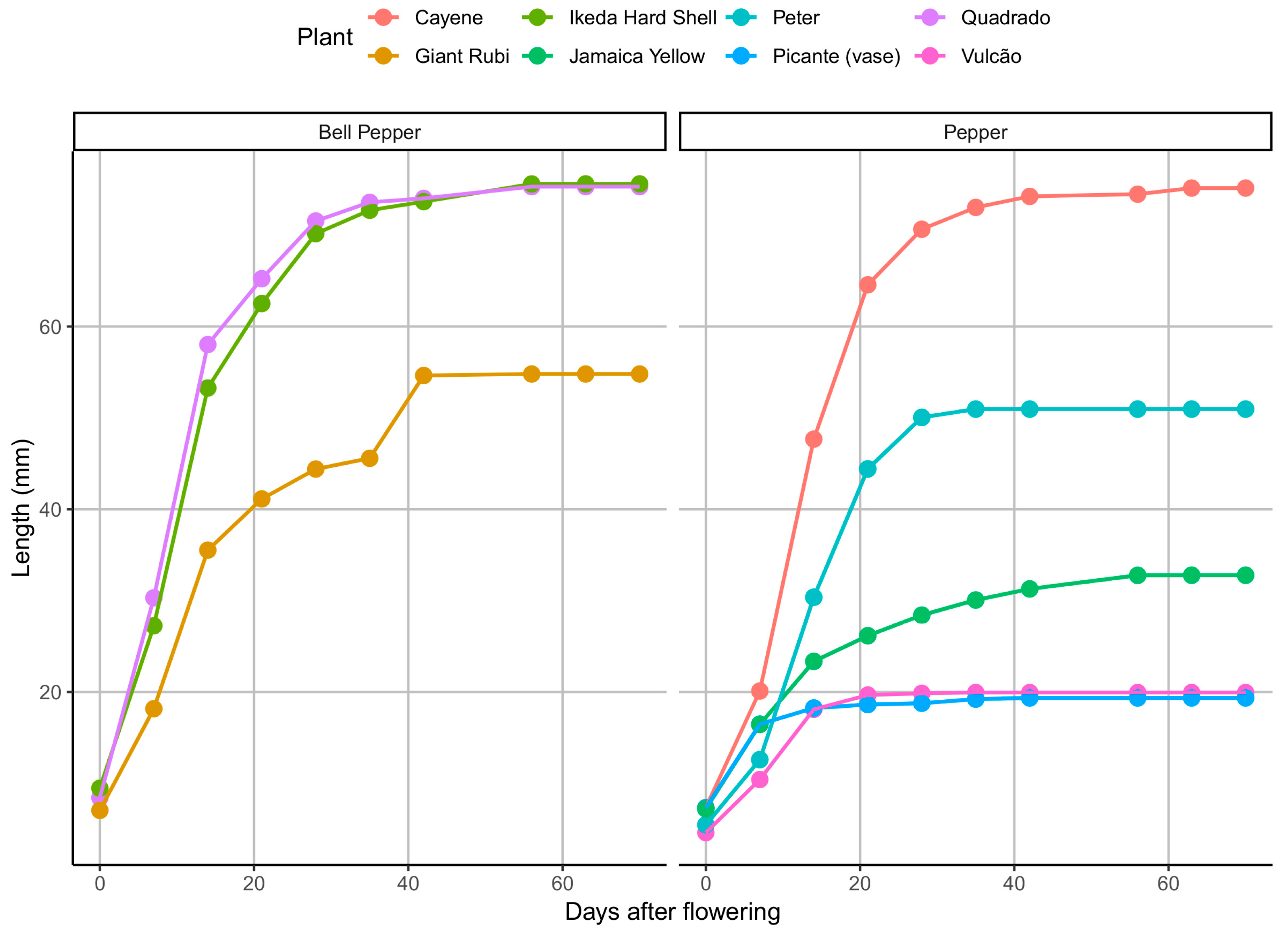
Figure 1 highlights the difference in length between the pepper and bell pepper groups that were considered for estimating the models’ fixed effects. The increase in fruit length occurs sharply until approximately the twentieth DAF, from where this difference between fruit types becomes clearer. The bell pepper species have an asymptotic length (at the end of the curve) higher than the pepper fruits (
Figure 1), with average results close to 60 mm and 45 mm, respectively.
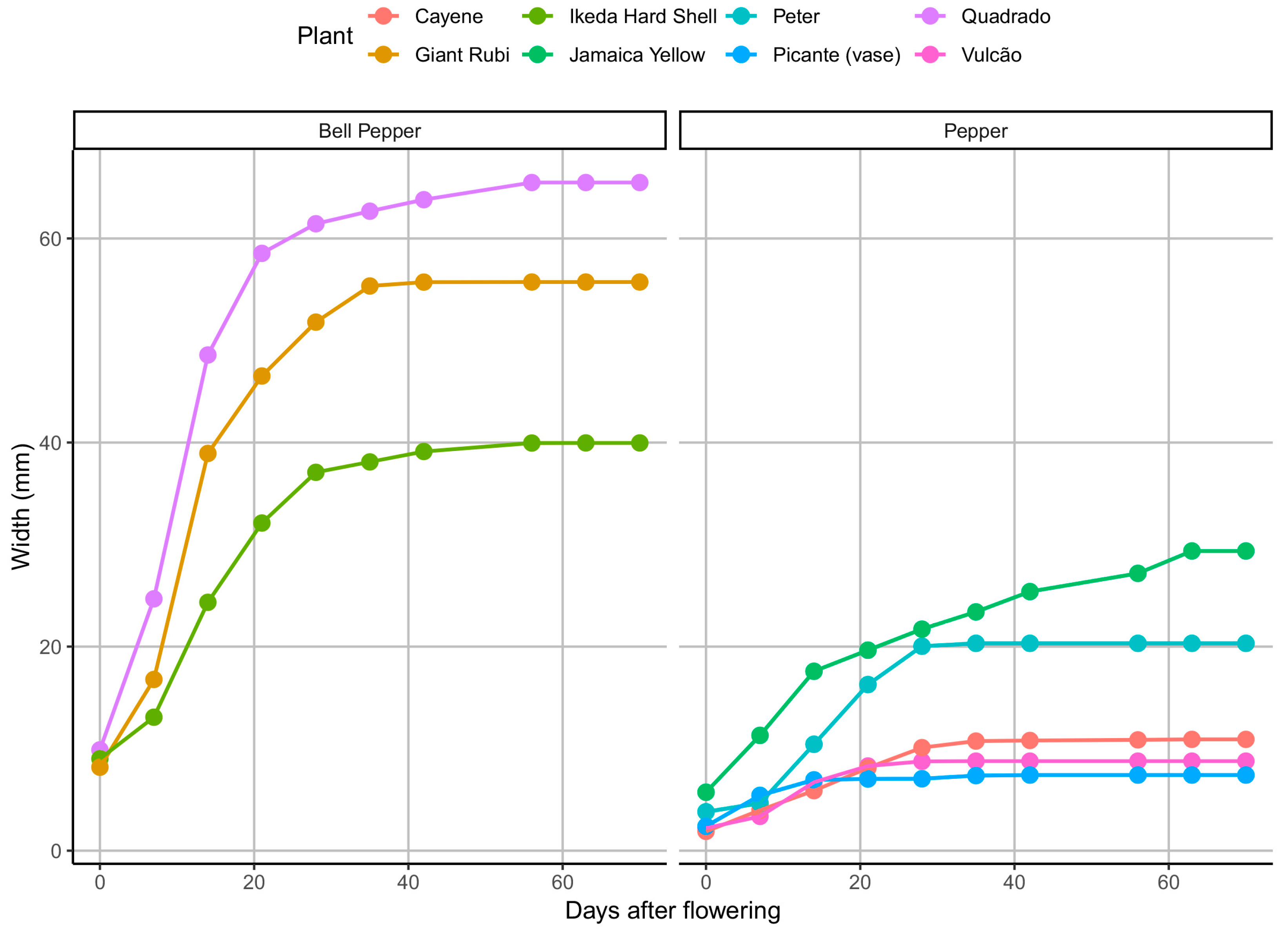
When the width of the fruits is descriptively analyzed (
Figure 2), the difference between types of pepper again occurs both in the shape of the curve, which is more pronounced for pepper fruits, and for the asymptotic width, with mean values close to 50 mm for bell peppers and less than 20 mm for peppers. For both groups, the growth in width occurs markedly until approximately the tenth DAF, from when it happens in a less obvious form.
Both for the length and for the width of the fruits, there was convergence in the estimation of parameters for all the models used. Analyzing the comparison between models for the adjustment of growth in fruit length, we can see that the Gompertz, Logistic, and Richards models presented similar results according to the measures of goodness of fit (
Table 3). The Richards equation presented the best results according to AIC (412.61), BIC (432.82), MSE (2.32), MAE (1.06) and
(0.9957), showing a difference with lower values for the other models, except for
. The Gompertz and Logistic models also proved efficient for such measures. The von Bertalanffy equation showed divergent results, distancing from the others in terms of goodness of fit, showing higher values of both MSE (226.24) and MAE (12.03), respectively. The other results of the model quality assessment can be found in
Table 3.
When observing the quality criteria of the models for adjusting the width of the fruits (
Table 4), the model that presented the best measures of quality of adjustment, in general, was the Logistic one, showing lower values of AIC, BIC, and MAE (339.61, 361.04 and 0.91, respectively). Analyzing the MSE and the
, the Richards model was superior (1.47 and 0.9960), despite presenting a slight difference from the Logistic model (1.50 and 0.9959). As in the length modeling, the two cited models and the Gompertz equation were superior in terms of goodness of fit compared to the von Bertalanffy one. The
for all models, except for the von Bertalanffy equation, showed an almost perfect fit, always greater than 0.9949 (
Table 4).
Considering the fixed-effects estimates (
’s) together with their standard errors (between parentheses) for the length-adjustment models (
Table 5), it is observed that the biologically interpretable parameters (
and
, respectively representing the asymptotic length and time to inflection point) are similar for all models. The asymptotic length was estimated for the group of peppers (
) ranging from 39.26 mm (Logistic) to 40.07 mm (von Bertalanffy), while for bell peppers, this parameter ranged from 66.95 mm (Logistic) to 68.48 mm.
The Richards model was considered the best for adjusting this variable and the others and could estimate the difference between the studied groups for all parameters compared between pepper and bell pepper (
Table 5). We can observe from the estimates of this model, for example, that bell pepper fruits have an asymptotic length (
) of 67.87 mm, while the asymptotic length for pepper (
) is close to 39.27 mm (
Table 5). The difference is smaller when we consider the time to the point of inflection of fruit length in pepper (
) and bell pepper (
), where growth is maximized at 7.72 and 6.43 days, respectively. Estimates of the other parameters, with their respective standard errors, can be seen in
Table 5.
Considering the parameter estimates for fruit width (
Table 6), the difference between the asymptotic-weight estimates of pepper and bell pepper is also evident, with width estimates varying around 15.50 and 53.50, respectively. The time to the inflection point is practically the same for both groups according to the Gompertz model (6.39 and 6.46, respectively) and shows similar estimates for the Logistic model (11.16 and 10.04, respectively), considered the best adjustment for this question. Therefore, according to this model, fruit-width growth is maximized at approximately 11 days for pepper fruits and ten days for bell peppers. The other results can be seen in
Table 6.
Considering the criteria used as a quality of fit, the Richards equation proved to be more efficient for fruit-length adjustment because it was superior in all the measures used, while the Logistic model stood out for better adjusting the width growth, being superior in terms of AIC, BIC, and MAE.
Figure 3 shows the proximity between the observed values (points) and the adjusted values (solid line) according to the Richards model for fruit-length growth. We can see that the solid line for pepper (in blue) and bell pepper (in red) shows how close the estimated values are to the actual values. There was also a high variation within groups, mainly in terms of asymptotic length. It is more clearly observed that the Ikeda Hard Shell and Quadrado peppers have a higher asymptotic length than most other plants, with estimates greater than 70 mm (
Figure 3). As for the same characteristic, the pepper fruits are smaller, with measurements close to 40 mm, except for the Cayenne pepper, the only pepper fruit that showed an asymptotic length greater than 60 mm.
Observing the curves adjusted by the Logistic model for fruit width (
Figure 4), there is a noticeable proximity between the observed values and the model (continuous lines) for pepper and bell pepper, represented by the same colors. The growth occurs more markedly among the bell pepper fruits, reaching higher length and width in general compared to the pepper fruits. It can be seen graphically that most fruits’ tipping point is approximately ten days. The average asymptotic width for the bell pepper fruits is higher than for the pepper fruits. As well as the asymptotic length adjustment, a high variation was also observed within the groups considering the model for width fit.
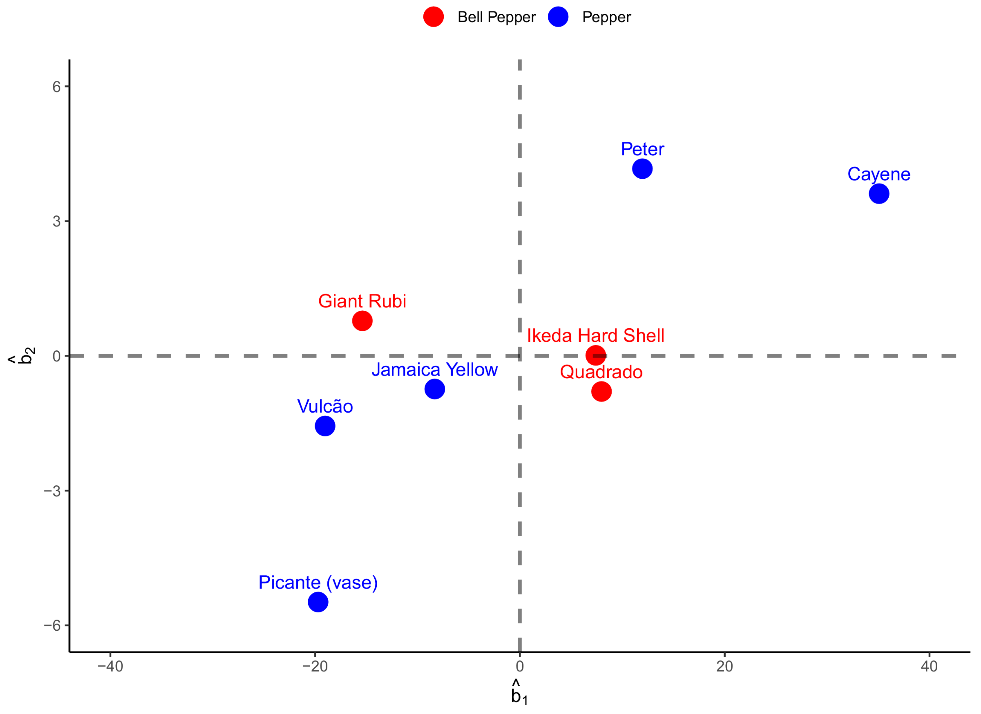
The relationship between the zero-centered individual random-effects estimates corresponding to the asymptotic length (
) and time to the inflection point (
) is shown in
Figure 5. The estimated Pearson correlation coefficient was 0.75, showing that regardless of the type of pepper, the relationship between these two growth parameters is positive and moderate. It can also be noted that individual differences between peppers of the same kind could be identified, such as the Cayenne and Peter peppers, which presented positive estimates indicating that they are above average for both
and
. Considering bell peppers, however, the variation was smaller in relation to peppers. Quadrado and Ikeda Hard Shell were superior in terms of asymptotic length. At the same time, Giant Rubi reached the curve’s inflection point more quickly (
Figure 5).
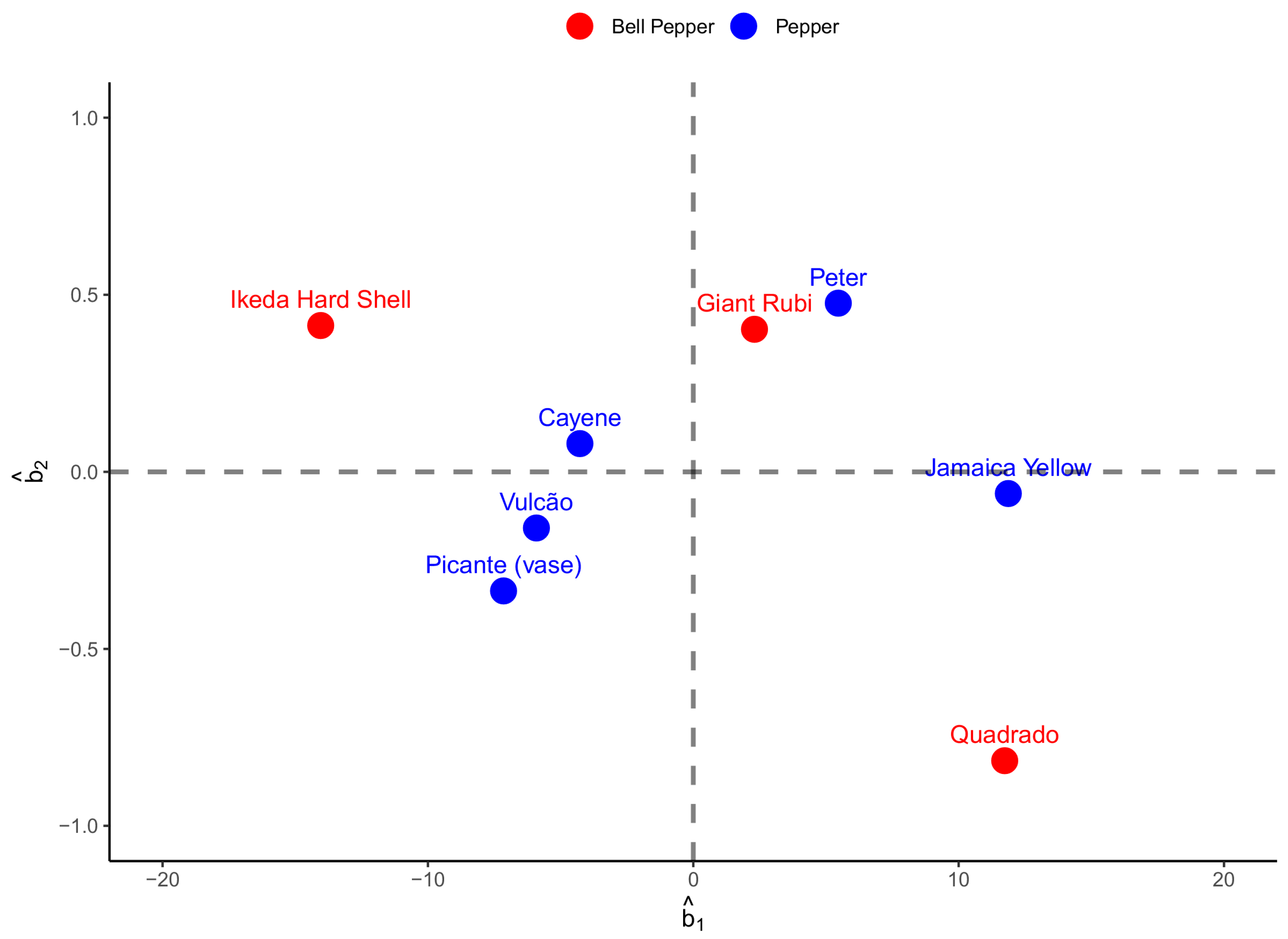
Considering the similar graph, now observing the analysis for width data (
Figure 6), we can identify the most pronounced variability among bell pepper fruits. The correlation between random effects, unlike what happened with the length model, showed an almost zero correlation of −0.02. The Jamaica Yellow pepper was superior to the others in the same group regarding asymptotic width, while the Peter pepper took longer to reach the inflection point. Ikeda Hard Shell was shown to be inferior to other peppers. However, it takes longer to reach the tipping point. The behavior of the Quadrado bell pepper could be better, obtaining prominence for the asymptotic width and less time to the inflection point. The other estimates of random effects for the biologically interpretable parameters can be seen in
Figure 6.
4. Discussion
When proposing the estimation method used in this work, Lindstrom and Bates [
5] highlighted that procedures for selecting and criticizing models need to be developed and studied using real data. The flexibility of this methodology using data from real experiments proved to be true when it was possible to include in the model fixed effects of the group of peppers (pepper and bell pepper) and individual random effects for the biologically interpretable variables (asymptotic length and width and time to the point of curve inflection). The efficiency in terms of prediction could be observed according to the low MSEs and MAEs observed in
Table 3 and
Table 4 and
Figure 3 and
Figure 4, which illustrate estimated curves close to the actual observations for the two groups for length adjustment and fruit width. This methodology efficiency corroborated with some works that obtained good results, such as applications for
eucalyptus spp. trees [
32], pepper [
7], Guzerá cattle [
10], dairy buffaloes [
11], dairy goats [
33], heifers [
34] and larch [
16]. This shows the effectiveness of the methodology in different contexts.
The difference between the growth patterns for both the length and width of pepper and bell pepper fruits is evidenced by observing
Figure 2 and
Figure 4, respectively. For the three bell pepper fruits, both the length and the asymptotic width (final part of the growth phase) show different results, with the same behavior observed for the growth rate, where it is noted that bell pepper fruits increase in size more sharply. This notorious difference in behavior between the two types of fruit reinforces the need to use NLME with the insertion of the kind of fruit as a fixed effect. To confirm this need, it is interesting to observe the results of
Table 5 and
Table 6, which show that, both for length and width adjustment, the average fixed-effect coefficients (
’s) presented different estimates between the groups, mainly in what concerns the asymptotic length and width, respectively, shown in
Table 5 and
Table 6. The difference between the width of pepper and bell pepper fruits is in accordance with what was observed by Rosado et al. [
35], who, using genotypes like those of this work, estimated that the mean fruit width of bell pepper was statistically greater than in pepper by the Scott-Knott test considering a nominal significance level of 5%. However, when analyzing length, peppers and bell peppers obtained similar measurements.
Analyzing the comparison of models for adjusting fruit-length growth (
Table 3), we can see that the best model in terms of all 5 measures of goodness of fit (AIC, BIC, MSE, MAE and,
) was that of Richards. This equation is the only one in this study that presents the coefficient
, which, according to Archontoulis and Miguez [
24], has the function of dealing with asymmetric growth. This fact suggests that the addition of this parameter was able to improve the adjustment efficiency both in terms of likelihood when observing the AIC and BIC and in terms of prediction (MSE and MAE and
). The improvement of the model also suggests that fruit-length growth occurs asymmetrically, reinforcing what was observed in the graphical analysis (
Figure 1), where the phenotypes reach the inflection point in approximately ten days. This can also be confirmed by looking at the estimates for the time to the tipping point for pepper (
) and pepper (
) in
Table 5. Still about the length characteristic, the efficiency of the Logistic model was corroborated by Oliveira et al. [
6], who observed that for three of the five pepper genotypes, the Logistic model was the best fit. In the comparison made by this work, however, the Richards model was not included.
Regarding the fruit width, the Logistic model presented more relevant results in terms of AIC, BIC, and MAE (
Table 3), in addition to values of MSE and
practically equal to those of the Richards model. This result shows that, despite having three parameters (one less than the Richards model), the Logistic model was the most efficient for describing the growth of this variable. This also shows that the fourth parameter of the Richards model, described earlier, did not make much difference in adjusting the fruit width since there were no gains compared to the Logistic model. Oliveira et al. [
6], also working with pepper width, observed that the Logistic model presented better AIC values for three of the five genotypes used when evaluating the fruits’ width, corroborating this work’s results. Other similar works studying fruit growth also concluded that the Logistic model stood out from the other studies [
8,
36,
37].
The proximity of zero estimated by the MSE was also found by other authors [
6], who used Quantile Regression and Ordinary Least Squares (OLS) for parameter estimation. The authors used an adjustment per individual considering fixed effects and included in the sample genotypes like those of pepper (first group) found in this work. Considering the same area, the Gompertz, Logistic and von Bertalanffy models adjusted the data satisfactorily, as in the present work.
We can observe that, for the comparison among models for both length and width, the equations showed differences between high AICs between the best and worst models. It is known according to [
38] that differences greater than 10 units in terms of AIC comparison between the best and worst models indicate that the one with the highest AIC is not suitable. Therefore, there is a reasonable difference in performance among the models studied on both occasions (
Table 3 and
Table 4). The good quality of fit with the type of pepper as a covariate also suggests that by adding other covariates in future work, such as thermal time, we may also find relevant results.
The estimates of parameter
and
, both for length and width, were close in all models studied, whereas, for the estimate of parameter
and
, more divergent results were obtained (
Table 3 and
Table 4). Considering
and
, in all traits, there was a similarity in the parameter estimates between the Gompertz, Logistic, Richards, and von Bertalanffy models. Similar results can be observed in work by Wen et al. [
39], who, using partridges, studied the body-weight curve using nine different nonlinear models, including four of the five used in our work. The authors obtained similar estimates of
and
among the Gompertz, Logistics, von Bertalanffy, and Richards models, whereas for
there were greater divergences of results when comparing the models.
The random effects of the parameters of the curves estimated by the Richards model for fruit length (
Figure 5) and Logistic for fruit width (
Figure 6) identify the individual estimates of these parameters for each genotype used. Looking at the relationship between asymptotic length (
) and time to the inflection point (
) in
Figure 5, we note a positive and strong relationship of 0.75, indicating that fruits that reach a higher asymptotic weight tend to require more time to reach the tipping point. It is also noted that the Peter and Cayenne species tend to have a greater difference in relation to the estimated average effects for the first group (pepper), with these differences being higher in this group. Looking at
Figure 6, we can see that the relationship between the asymptotic width (
) and the time to the inflection point (
) is close to zero correlation, with a value of −0.02. This result indicates that contrary to fruit length, there is no association between these variables when analyzing fruit width, indicating that the increase in asymptotic width is unrelated to time until the inflection point. As these are random effects derived from individual estimates of pepper fruits, regardless of the groups they are part of in this study, this result indicates that fruits that reach the inflection point more quickly will not necessarily have a high asymptotic weight. This represents the opposite of what happens if we consider the relationship between these variables for fruit length. It is also worth mentioning that in this case, there was a greater variation associated with group 2 (bell peppers).


 ,
, 


