Integrating Unmanned Aerial Vehicle-Derived Vegetation and Texture Indices for the Estimation of Leaf Nitrogen Concentration in Drip-Irrigated Cotton under Reduced Nitrogen Treatment and Different Plant Densities

Abstract

The accurate assessment of nitrogen (N) status is important for N management and yield improvement. The N status in plants is affected by plant densities and N application rates, while the methods for assessing the N status in drip-irrigated cotton under reduced nitrogen treatment and different plant densities are lacking. Therefore, this study was conducted with four different N treatments (195.5, 299, 402.5, and 506 kg N ha⁻¹) and three sowing densities (6.9 × 10⁴, 13.8 × 10⁴, and 24 × 10⁴ plants ha⁻¹) by using a low-cost Unmanned Aerial Vehicle (UAV) system to acquire RGB imagery at a 10 m flight altitude at cotton main growth stages. We evaluated the performance of different ground resolutions (1.3, 2.6, 5.2, 10.4, 20.8, 41.6, 83.2, and 166.4 cm) for image textures, vegetation indices (VIs), and their combination for leaf N concentration (LNC) estimation using four regression methods (stepwise multiple linear regression, SMLR; support vector regression, SVR; extreme learning machine, ELM; random forest, RF). The results showed that combining VIs (ExGR, GRVI, GBRI, GRRI, MGRVI, RGBVI) and textures (VAR, HOM, CON, DIS) yielded higher estimation accuracy than using either alone. Specifically, the RF regression models had a higher accuracy and stability than SMLR and the other two machine learning algorithms. The best accuracy (R² = 0.87, RMSE = 3.14 g kg⁻¹, rRMSE = 7.00%) was obtained when RF was applied in combination with VIs and texture. Thus, the combination of VIs and textures from UAV images using RF could improve the estimation accuracy of drip-irrigated cotton LNC and may have a potential contribution in the rapid and non-destructive nutrition monitoring and diagnosis of other crops or other growth parameters.

1. Introduction

Nitrogen (N) is normally required more than other nutrients for cotton growth, and the optimal application rate or ratio of N fertilizers is vital for cotton production and environmental sustainability [1]. However, excessive N application leads to growth and late maturity, while insufficient N affects development and yield formation [2,3]. Therefore, precise, real-time, and rapid detection of cotton’s N nutrient status is beneficial for quantifying N fertilizer management and promoting environmental friendliness.

Traditional nitrogen detection methods, based on direct chemical analysis, largely depend on field measurements and destructive sampling. Although these methods offer adequate measurement precision, their destructive nature, time-consuming processes, and labor-intensive characteristics limit their application on a large scale [4]. Remote sensing (RS) technology is primarily used in crop N monitoring due to its rapid, non-destructive characteristics [5,6]. Unmanned aerial vehicle (UAV)-based RS platforms are widely used in different crop fields for data collection and monitoring, owing to their low-cost and high spatio-temporal resolution [7,8,9,10].

The RGB, color infrared (CIR), multi-spectral, and high-spectral images derived from different sensors have been obtained and used on various UAV platforms to analyze crop growth conditions [11]. In particular, low-cost UAV systems with RGB or modified CIR sensors have been widely used for crop N content and biomass estimation [12,13,14]. RGB indices utilize basic color channels to provide a direct visual representation of crop health and stress, effectively capturing phenological changes such as color variations indicative of plant conditions. These indices are particularly useful in identifying shifts in plant growth, although their effectiveness may be limited under closed canopy or dense tree canopy cover [14,15]. However, the N status is strongly influenced by growth stages, and the poor correlation between LNC and RGB image parameters or vegetation indices was observed under higher plant densities [15]. Even more, the N signal of crop leaves and plants is hardly captured by canopy spectra at early growth stages, resulting from multiple background factors (e.g., water, soil, mulch) and N dilution effects. Previous studies found that the degree of N dilution in winter wheat was more obvious in the late growth stage than that in the earlier growth stage [16,17]. Therefore, there is little knowledge about how to enhance the N signal with lower or higher levels of crop canopy, and how to build up an appropriate model for N status for whole growth stages.

In response to these challenges, the integration of RGB and texture indices in UAV-based remote sensing presents a promising approach. Texture features, derived from UAV imagery, can precisely compensate for the limitations posed by conventional vegetation indices (VIs) under dense canopy conditions [18]. Conversely, texture indices, derived from the spatial arrangement and variation frequency of pixel intensities in UAV imagery, offer insights into plant density, leaf area index (LAI), and the complex three-dimensional structure of crop canopies [19,20]. These texture features compensate for the limitations of traditional vegetation indices (VIs), particularly under dense canopy conditions. They have proven to be more accurate and sensitive in reflecting the biophysical variables of crops compared to VIs. Especially during early growth stages, texture metrics can effectively capture significant color changes in leaves, often due to nitrogen uptake from fertilization and growth, thus providing a nuanced understanding of crop nitrogen status [21].

The possible and better data fusion depends on the availability of various data sources [22]. Data fusion enabled a more complete interpretation of the connection between remote sensing data and crop parameters [21,23]. Research has shown that the fusion of the spectral and texture information derived from UAV images could improve the predictive performance of crop biomass [19]. Since VIs and textures have their own advantages responding to crop parameters under different growth stages and plant densities, combining their complementary information may help to improve the estimation of crop parameters across the critical growth stages. For example, the fusion of VIs and texture data approaches has been utilized in estimating the aboveground biomass of wheat [18], quantification of the nitrogen (N) status of rice crop [19], estimating the height of the canopy and aboveground biomass of maize [14], etc. The fused data performed better than single data for crop parameter estimation; however, the results found that most of the remote sensing parameters and crop parameters did not have simple linear relationships. Linear models have limitations in handling complex data, such as the difficulty in capturing nonlinear relationships, sensitivity to outliers, and the assumption of independence among features [24]. Machine learning effectively improves these shortcomings by introducing nonlinear models, ensemble learning methods, feature engineering, regularization techniques, and adaptive optimization algorithms, making models more suited to handling complex data structures in the real world [25]. Compared to traditional linear regression techniques, machine learning regression algorithms can produce higher accuracy in biomass estimation. Machine learning regression algorithms have the advantages of dealing with high-dimensional data and nonlinear relationships, which can produce higher accuracy in biomass estimation compared to traditional linear regression techniques [14,26]. Among them, random forest (RF) [27], support vector regression (SVR) [28], and extreme learning machines (ELMs) [29] are widely used for crop parameter estimation. As far as we know, few studies have explored machine learning techniques to estimate the LNC of cotton by combining VIs and texture structure information from UAV images. Therefore, whether using machine learning algorithms to estimate drip-irrigated cotton LNC in textures and VIs has a better performance needs to be further explored.

Therefore, the aims of this study were (1) to assess the potential of combining VIs and texture information derived from a low-cost UAV-mounted RGB sensor to enhance the accuracy of estimating LNC in cotton; and (2) to assess the estimation performance of three machine learning regression techniques (SVR, ELM, RF) compared to the traditional stepwise multiple linear regression (SMLR) throughout the cotton growth stages under different plant densities and reduced N treatments. The anticipated results will guide how to choose an inexpensive way to perform N estimation and lay the groundwork for the development of non-destructive, rapid monitoring of nitrogen status using UAVs for cotton crops.

2. Materials and Methods

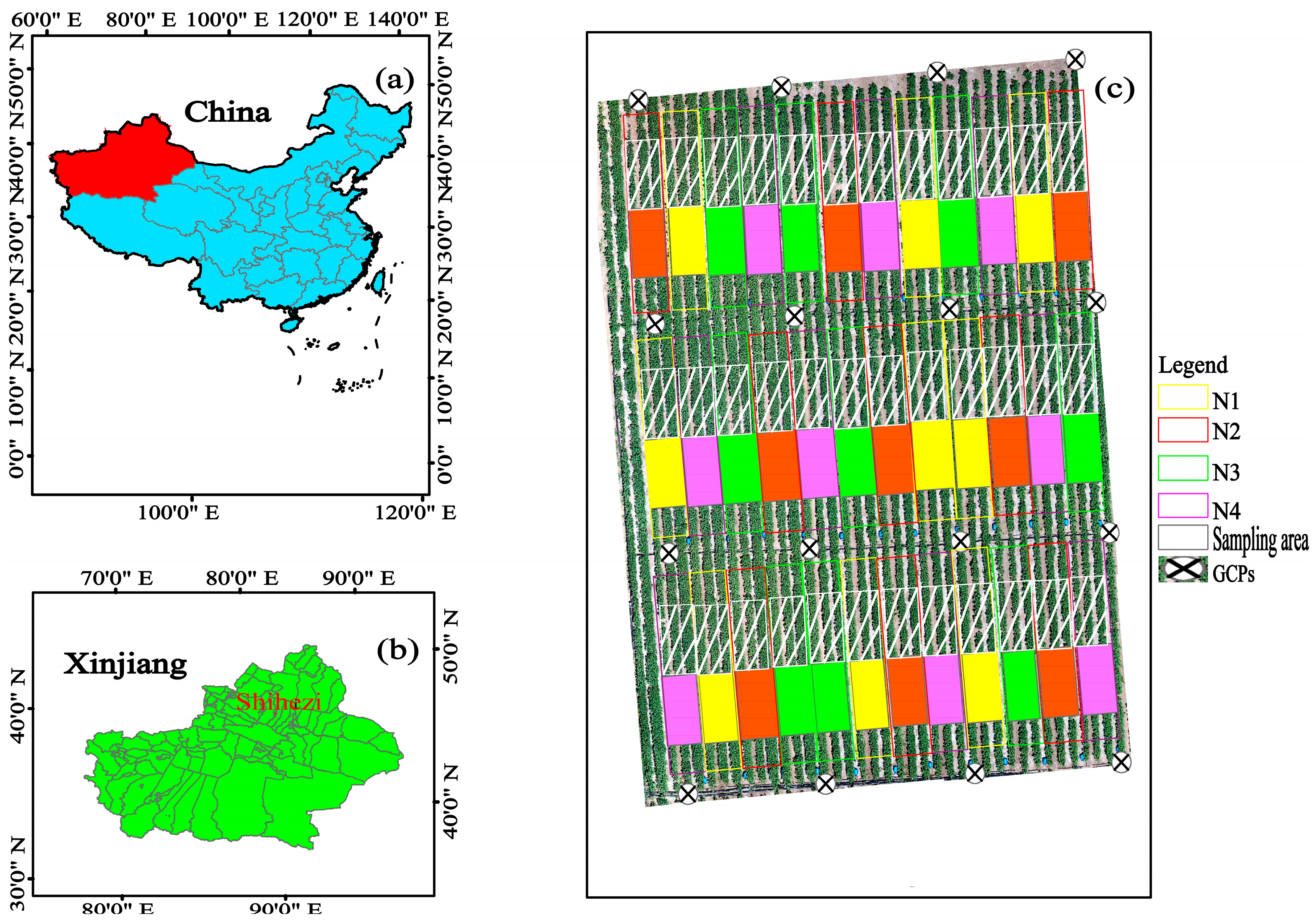
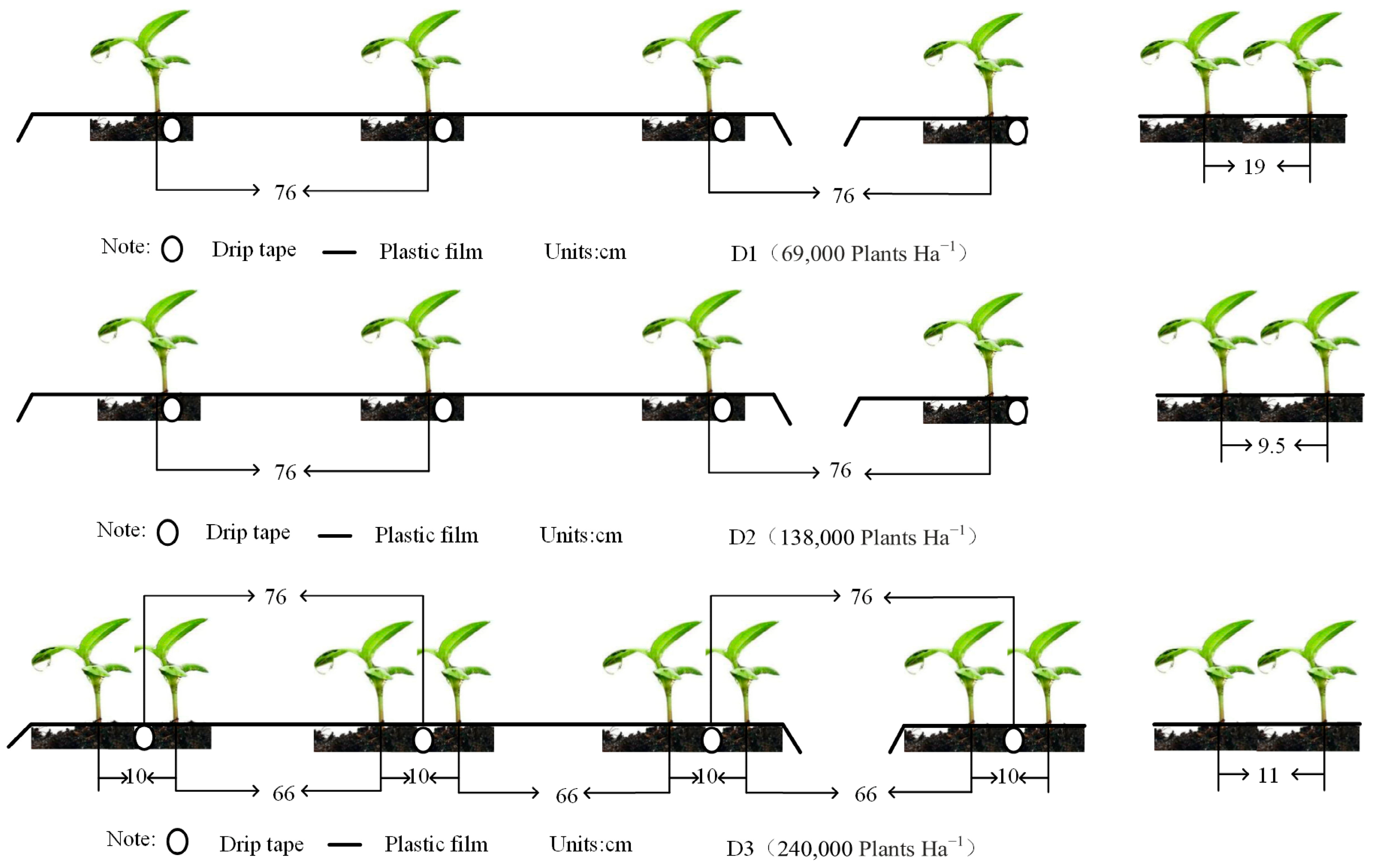
2.1. Experimental Design

The experiment was conducted in Shihezi University Experiment Base, Shihezi, Xinjiang, China (44°29″ N, 86°1″ E) in 2019 and 2020. The average temperature/rainfall for both years was 20 °C/168 mm and 21 °C/228 mm during the cotton-growing season, respectively. Four different levels of N treatment (195.5, 299, 402.5, and 506 kg N ha⁻¹) and three levels of densities (6.9 × 10⁴, 13.8 × 10⁴, and 24 × 10⁴ plants ha⁻¹) were conducted using hybrid cotton cultivar Lumianyan24. Treatments were laid out in a split-plot design: plant density as the main plot factor and nitrogen levels as the sub-plot factor, replicated three times (Figure 1). In the high-density pattern, cotton was planted in six rows with three irrigation pipes, covered by a 2.05 m wide plastic film, spaced at 11 cm intervals. The low- and medium-density planting pattern is one film with three rows and three drip tapes with a plant spacing of 9.5 and 19 cm, respectively (Figure 2). The details of the basic soil fertility of the experiment plot can be found in Appendix A 

Table A3. Basic fertility in experimental plot.

Year	Hydrolyzable N (mg kg−1)	Olsen-P (mg kg−1)	Available-K (mg kg−1)	Organic Matter (g kg−1)	pH
2019	186.7	78.7	332.0	21.9	7.82
2020	44.3	19.0	486.0	15.5	8.17

. The area of each plot was 34.2 m² (15 × 2.28), for a total of 36 plots; all other agricultural practices were performed based on local standards.

2.2. Ground Sampling and UAV Data Acquisition and Pre-Processing

The ground destructive samplings and UAV campaigns were undertaken at critical growth stages of cotton (

Table 1. Details of field campaigns for this study.

Experiment	Sowing Date	Date of UAV Flights	Date of Field Sampling	Growth Stage
#1	24 April 2019	1 July 2019	1 July 2019	Full bud stage
		16 July 2019	16 July 2019	Full flowering stage
		7 August 2019	7 August 2019	Early full-bolling stage
		16 August 2019	16 August 2019	Late full-bolling stage
		7 September 2019	8 September 2019	Boll opening stage
#2	18 April 2020	14 June 2020	15 June 2020	Full bud stage
		4 July 2020	4 July 2020	Full flowering stage
		27 July 2020	27 July 2020	Full-bolling stage
		21 August 2020	21 August 2020	Late full-boll stage
		13 September 2020	13 September 2020	Boll opening stage

). After the UAV campaign, three cotton plants were randomly sampled in each plot and divided into three parts including leaves, stems, and reproductive organs. The samples were then oven-dried at 105 °C for 30 min, followed by drying at 80 °C until a constant weight was achieved. Afterward, the dry samples were weighed, ground, and passed through a 0.5 mm sieve to evaluate the plant N content. The method used for N content assessment was the micro-Kjeldahl method [30].

The UAV system used was the DJI Mavic Pro series, equipped with a four-rotor setup and a digital camera. Before the preliminary flight, 16 ground control points (GCPs) were established throughout the cotton field experiment site, each marked with a sign, to georeference the UAV images taken at different growth stages, and the Real-Time Kinematic Global Positioning System (RTK-GPS, CHC X900 GNSS) with vertical and horizontal errors within 2 cm and 1 cm was used to acquire the original geographic coordinates.

In our campaign, the UAV with auto-flight mode and predefined operational plan was set to acquire RGB images with about 82% forward and lateral overlap, and the frequency of image acquisition was 1 frame per 5 s and the images were saved in JPEG format. In addition, the setting of the aperture of the camera was f/5, and the flight height was 10 m above the ground at the speed of 2 ms⁻¹. Throughout the season’s drone activities, all parameters related to the camera and drone (except exposure time) remained the same, with the specific parameters listed in

Table A1. Camera and UAV Parameters.

Camera	Parameters	UAV	Parameters
Resolution	4000 × 3000	UAV name	DJI-Mavic Pro
Image DPI	72 dpi	Flying height	10 m
Bit depth	8	Flying Speed	2 m/s
Aperture	f/5	Takeoff weight	734 g
Exposure	1/1250 s
ISO	ISO-1600
Focal length	26 mm
Field of view	64°

. All parameters (except the exposure time) related to the camera and UAV were the same during the UAV campaign in whole seasons. Each fight campaign was conducted on a sunny day between 12:00 p.m. and 14:00 local time and approximately 289 images were acquired with a ground resolution of 1.3 cm.

The Agisoft Photoscan 1.2.6 (Agisoft LLC, St. Petersburg, Russia) software was used to process the UAV images to obtain orthophotos. The detailed image-processing methodology that we used in this study was that utilized by Lu et al. (2019) [14], and the processing steps and parameter settings can be found in

Table 2. Processing steps with corresponding parameter settings in Agisoft Photoscan software for generation of orthophotos from UAV imagery.

Task	Parameter Setup
Aligning image	Accuracy: high; Pair selection: generic; Key points: 40,000; Tie points: 4000
Building mesh	Surface type: height field Source data: dense cloud; Face count: high
Positioning guided marker	Manual positioning of markers on the even 16 GCPs for all the photos
Optimizing cameras	Default settings
Building dense point cloud	Quality: high; Depth filtering: mild
Building texture	Mapping mode: Generic; Blending mode: Mosaic; Texture size/count: 4096
Building DEM	Surface: Mesh; Other parameters: default
Building orthomosaic	Surface: Mesh; Other parameters: default

.

2.3. Selection of Image Textures

The image textures based on the gray-tone spatial-dependence matrix (

Table 3. Detailed information of textures, calculation window size, and image ground resolution in this study.

Textures and Abbreviations	Bands	Windows	Ground Resolutions
Variance (VAR), Entropy (EN), Correlation (COR),	R, G, B	3 × 3	1.3 cm, 2.6 cm, 5.2 cm,
Homogeneity (HOM), Second Moment (SE),			10.4 cm, 20.8 cm, 41.6 cm,
Dissimilarity (DIS), Contrast (CON), Mean (MEA)			83.2 cm, 166.4 cm

), used in this study, were defined by Haralick [31]. The calculation formulas of eight image textures were related to all three bands in RGB images using a 3 × 3 calculation window. The textures in Table 3 are calculated by using

$$\mathrm{VAR}={\displaystyle \sum _{\mathrm{i}}{\displaystyle \sum _{\mathrm{j}}{\left(\mathrm{i}-\mathrm{u}\right)}^2\mathrm{p}\left(\mathrm{i},\mathrm{j}\right)}},$$

(1)

$$\mathrm{HOM}={\displaystyle \sum _{\mathrm{i}}{\displaystyle \sum _{\mathrm{j}}\frac{1}{1+{(\mathrm{i}-\mathrm{j})}^2}}}\mathrm{p}(\mathrm{i},\mathrm{j}),$$

(2)

$$\mathrm{CON}={\displaystyle \sum _{\mathrm{n}=0}^{{\mathrm{N}}_{\mathrm{g}}-1}{\mathrm{n}}^2\left\{\left.{\displaystyle \sum _{\mathrm{i}=1}^{{\mathrm{N}}_{\mathrm{g}}}{\displaystyle \sum _{\begin{array}{l}\mathrm{j}=1\\ \left|\mathrm{i}-\mathrm{j}\right|=\mathrm{n}\end{array}}^{{\mathrm{N}}_{\mathrm{g}}}\mathrm{p}(\mathrm{i},\mathrm{j})}}\right\}\right.},$$

(3)

$$\mathrm{EN}=-{\displaystyle \sum _{\mathrm{i}}{\displaystyle \sum _{\mathrm{j}}\mathrm{p}(\mathrm{i},\mathrm{j})}}\log \left(\mathrm{p}\left(\mathrm{i},\mathrm{j}\right)\right),$$

(4)

$$\mathrm{SE}={\displaystyle \sum _{\mathrm{i}}{\displaystyle \sum _{\mathrm{j}}\left\{\mathrm{p}(\mathrm{i},\mathrm{j}\right.}}{\left.)\right\}}^2,$$

(5)

$$\mathrm{MEA}={\displaystyle \sum _{\mathrm{i}=2}^{2{\mathrm{N}}_{\mathrm{g}}}\mathrm{i}{\mathrm{p}}_{\mathrm{x}+\mathrm{y}}}(\mathrm{i}),$$

(6)

$$\mathrm{COR}=\frac{{\displaystyle {\sum }_{\mathrm{i}}{\displaystyle {\sum }_{\mathrm{j}}(\mathrm{i},\mathrm{j})\mathrm{p}(\mathrm{i},\mathrm{j})-{\mathrm{u}}_{\mathrm{x}}{\mathrm{u}}_{\mathrm{y}}}}}{{\mathsf{\sigma }}_{\mathrm{x}}{\mathsf{\sigma }}_{\mathrm{y}}},$$

(7)

$$\mathrm{DIS}={\displaystyle \sum _{\mathrm{n}=1}^{{\mathrm{N}}_{\mathrm{g}}-1}\mathrm{n}\left.\left\{\begin{array}{c}{\displaystyle \sum _{\mathrm{i}=1}^{{\mathrm{N}}_{\mathrm{g}}}{\displaystyle \sum _{\mathrm{j}=1}^{{\mathrm{N}}_{\mathrm{g}}}\mathrm{p}(\mathrm{i},\mathrm{j})}}\\ \left|\mathrm{i}-\left.\mathrm{j}\right|=\mathrm{n}\right.\end{array}\right.\right\}},$$

(8)

where p(i, j) is the (i, j) entry in a normalized gray-tone spatial-dependence matrix P(i, j)/Rp_x(i)[=P(i, j))/R]; p_x(i) is the entry in the marginal-probability matrix obtained by summing the rows of p(i, j)${\displaystyle {\sum }_{\mathrm{j}=1}^{{\mathrm{N}}_{\mathrm{g}}}\mathrm{p}(\mathrm{i},\mathrm{j})}{\mathrm{N}}_{\mathrm{g}}\mathrm{p}(\mathrm{i},\mathrm{j})={\displaystyle {\sum }_{\mathrm{j}=1}^{{\mathrm{N}}_{\mathrm{g}}}\mathrm{p}(\mathrm{i},\mathrm{j})}$. N_g is the number of distinct gray levels in the quantized image; p_y(j)$={\displaystyle {\sum }_{\mathrm{j}=1}^{{\mathrm{N}}_{\mathrm{g}}}}$p(i, j)p_y(j)$={\displaystyle {\sum }_{\mathrm{j}=1}^{{\mathrm{N}}_{\mathrm{g}}}}$p(i, j); and u_x, u_y, σ_x, and σ_y are the means and standard deviations of p_x and p_y. Further details of the calculations can be found in Haralick [30].

2.4. Selection of Vegetation Indices

Ten vegetation indices of the RGB images were used to estimate the LNC in this study (

Table 4. Summary of vegetation indices derived from the aerial orthophotos for the estimation of LNC in cotton.

Index	Name	Formulation	References
IKAW	Kawashima Index	$\mathrm{IKAW}=\frac{\mathrm{R}-\mathrm{B}}{\mathrm{R}+\mathrm{B}}$	[31]
RGBVI	Red Green Blue Vegetation Index	$\mathrm{R}\mathrm{G}\mathrm{B}\mathrm{V}\mathrm{I}=\frac{{\mathrm{G}}^2-\mathrm{B}\ast \mathrm{R}}{{\mathrm{G}}^2+\mathrm{B}\ast \mathrm{R}}$	[32]
MGRVI	Modified Green Red Vegetation Index	$\mathrm{M}\mathrm{G}\mathrm{R}\mathrm{V}\mathrm{I}=\frac{{\mathrm{G}}^2-{\mathrm{R}}^2}{{\mathrm{G}}^2+{\mathrm{R}}^2}$	[19]
GLI	Green Leaf Index	$\mathrm{G}\mathrm{L}\mathrm{I}=\frac{2\ast \mathrm{g}-\mathrm{r}-\mathrm{b}}{2\ast \mathrm{g}+\mathrm{r}+\mathrm{b}}$	[33]
ExGR	Excess Green minus Excess Red	$\mathrm{E}\mathrm{x}\mathrm{G}\mathrm{R}=\mathrm{E}\mathrm{x}\mathrm{G}-\frac{1.4\mathrm{R}-\mathrm{G}}{\mathrm{G}+\mathrm{R}+\mathrm{B}}$	[34]
GRVI	Green Red Vegetation Index	$\mathrm{G}\mathrm{R}\mathrm{V}\mathrm{I}=\frac{\mathrm{G}-\mathrm{R}}{\mathrm{G}+\mathrm{R}}$	[35]
ExG	Excess Green Index	$\mathrm{E}\mathrm{x}\mathrm{G}=2\ast \mathrm{g}-\mathrm{r}-\mathrm{b}$	[36]
VARI	Visible Atmospherically Resistant Index	$\mathrm{V}\mathrm{A}\mathrm{R}\mathrm{I}=\frac{\mathrm{g}-\mathrm{r}}{\mathrm{g}+\mathrm{r}-\mathrm{b}}$	[37]
GBRI	Green blue ratio index	$\mathrm{G}\mathrm{B}\mathrm{R}\mathrm{I}=\frac{\mathrm{G}}{\mathrm{B}}$	[38]
GRRI	Green red ratio index	$\mathrm{G}\mathrm{R}\mathrm{R}\mathrm{I}=\frac{\mathrm{G}}{\mathrm{R}}$	[39]

Note: R, G, and B represent the digital number of red, green, and blue channels, respectively. r = R/(R + G + B), g = G/(R + G + B), b = B/(R + G + B).

), and the selected VIs were based on the three bands of the original RGB images.

2.5. Regression Modeling Methods

Compared to traditional parametric regression methods, machine learning algorithms would be more suitable for predictive model building for multiple input variables. For building an independent model based on LNC estimation using VIs, textures, and their combinations, three machine learning techniques were used and realized via the Rx64 3.4.0 environment software in conjunction with the caret package (R Development Core Team, 2017).

Random Forest (RF) is a non-linear integrated modeling method with multiple decision trees, and consists of Bootstrap and random subspace methods [27]. Based on this, it shows a better capability to overcome the overfitting problems and to handle small datasets, as well as handling a massive number of input variables [14,38]. Mtry and ntree were used in RF to attain the best predictive power, and the ntree was fixed to 1300 and mtry was only adjusted to optimize the RF model in this study.

An extreme learning machine (ELM), a single hidden layer feed-forward neural network, offers faster learning speed, lower training error, and minimal output weight specifications compared to traditional networks [29,40]. It is suitable for real-time training as the weights of its hidden layer may be generated randomly without any iteration optimization. Moreover, an ELM has a better capability to handle complex data and develop regression with multiple highly.

Support vector machine (SVM) is a very powerful machine learning regression approach based on statistical theory, and is usually used for pattern recognition and nonlinear regression [41,42]. SVR has been widely used in previous remote sensing studies to estimate crop parameters [43] due to its ability to handle high-dimensional data and train models with a relatively small number of samples [28]. In this study, each SVM model automatically estimated a fixed σ value for every input variable according to the kernel-based machine learning regression methods provided by the R package “kernlab” [43]. The Cost was further tuned to optimize the predictive performance of the SVM model.

Stepwise multiple linear regression (SMLR) is a commonly used regression method in relation to crop growth parameters [24]. The variables extracted from the UAV images may be interrelated, and the relationships among each variable and the relationships between these variables with LNC were subjected to simple linear regression as measured using Pearson’s correlation coefficient. Moreover, to better assess the performance of three machine learning algorithm methods using traditional regression techniques, SMLR was used as a reference in this assessment.

2.6. Accuracy Assessment

The objective was to build a generalized model across multi-treatment, growth periods, and seasons using various regression techniques, and we pooled 2 years of data under all growth conditions to form a holistic dataset. A generalized model would be more practical than a local model on account of avoiding frequent model calibration for different growth conditions. The dataset was split into two parts: 70% for model calibration and 30% for validation. The coefficient of determination (R²), the root mean square error (RMSE), and the akaike information criterion (AIC) were used to evaluate the accuracy of model calibration. The estimation accuracy was evaluated using R², RMSE, average test prediction accuracy (ATPA), and relative RMSE (rRMSE) of the validation data. The ATPA was calculated as follows:

$$\mathrm{ATPA}=\left(1-\frac{1}{\mathrm{N}}\sum _{\mathrm{i}=1}^{\mathrm{N}}\frac{\left|{\mathrm{T}}_{\mathrm{A}}-{\mathrm{T}}_{\mathrm{P}}\right|}{{\mathrm{T}}_{\mathrm{A}}}\right)\times 100$$

(9)

where T_A is the observed value, T_P is the predicted value, N is the number of observations, and $\left|{\mathrm{T}}_{\mathrm{A}}-{\mathrm{T}}_{\mathrm{P}}\right|$ is the absolute error between the actual value and the predicted value.

3. Results

3.1. Correlation between LNC, Vis, and Texture

We analyzed the changes in digital numbers (DN) across different channels corresponding to variations in LNC from the RGB image (Figure 3a). The DN values in all channels were slightly increased when LNC increased to 4.25%, and then decreased to be flatter as LNC increased. The DN values in the green channel were higher than those in the blue channel. Further, Figure 3b illustrates the correlation between UAV-derived vegetation indices (from 1.3 cm ground-resolution images) with LNC, and stronger positive correlations were observed in RGBVI, ExGR, ExG, and GLI with Pearson correlation coefficient values above 0.7. Normal R, G, and B were weakly negatively correlated with LNC and their Pearson correlation coefficient values were below −0.5.

For texture-related variables, most of the image textures in the three channels were strongly correlated with LNC in the five individual growth stages, and the correlation coefficients of the same texture metrics in each channel were close to LNC. During the whole growth stages, only VAR, CON, and DIS had high correlation coefficients with LNC, and they performed consistently under three channels (Figure 4). Thus, we selected high correlation coefficients (>0.6) variables GLI, ExG, ExGR, GRVI, GBRI, GRRI, MGRVI, and RGBVI variables in the VI group, and VAR, HOM, CON, and DIS in all three channels in the texture group for model development.

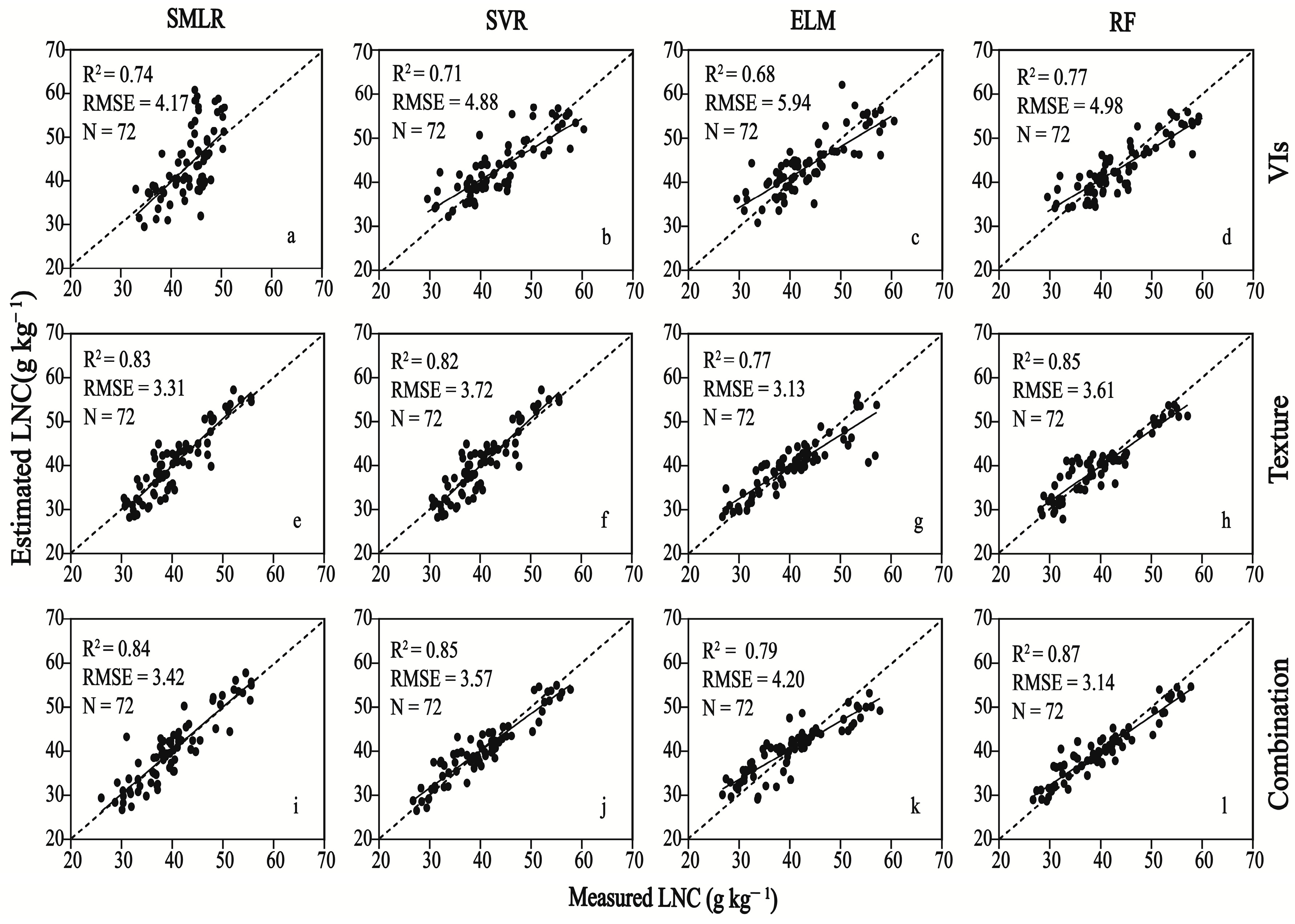
3.2. Comparison of LNC Estimation Performance among SMLR and Machine Learning Techniques

Table 5. Accuracy assessment for the estimation of LNC from vegetation indices, texture, and their combinations with SMLR and three machine learning algorithms.

Input Variables	Technique	Calibration (N = 288)			Validation (N = 72)
		R2	RMSE (g/Kg)	AIC	R2	RMSE (g/Kg)	rRMSE (%)
VIs	SMLR	0.72	4.11	680.61	0.74	4.17	12.78
	SVR	0.70	4.12	410.19	0.71	4.88	9.43
	ELM	0.68	4.25	408.50	0.68	5.94	9.72
	RF	0.76	3.72	414.83	0.77	4.98	8.51
Textures	SMLR	0.83	3.21	678.53	0.83	3.31	8.05
	SVR	0.82	3.17	386.96	0.82	3.72	7.89
	ELM	0.77	3.66	425.28	0.77	3.13	9.10
	RF	0.85	2.85	378.59	0.85	3.61	7.09
VIs and Textures	SMLR	0.84	3.11	678.53	0.84	3.42	7.75
	SVR	0.83	3.13	386.96	0.85	3.57	7.79
	ELM	0.78	3.63	425.28	0.79	4.20	9.04
	RF	0.87	2.80	378.59	0.87	3.14	7.00

Note: The accuracy metrics were calculated from calibration data and validation data separately. The number in bold for each column represents the maximum R², minimum RMSE, minimum AIC, and minimum rRMSE, respectively.

presents the comparison of SMLR, SVR, ELM, and RF for LNC estimation throughout the growth stages of cotton. The results indicate that using VIs alone, RF obtained the optimal calibration (R² = 0.76, RMSE = 3.72 g kg⁻¹, AIC = 414.83) and validation (R² = 0.77, RMSE = 4.98 g kg⁻¹, rRMSE = 8.51%) with performance across the four regression techniques. However, SMLR also showed high accuracy (validation: R² = 0.74, RMSE = 4.17 g kg⁻¹, rRMSE = 12.78%) and was competitive with RF. When using the textures alone, the best performance remained for RF, with a very close performance for SMLR and SVR. In contrast, ELM exhibited lower accuracy than that of SMLR, and RF achieved the highest level of accuracy among the four regression techniques. Furthermore, this accuracy with RF (Calibration: R² = 0.85, RMSE = 2.85 g kg⁻¹, AIC = 378.59; validation: R² = 0.85, RMSE = 3.61 g kg⁻¹, rRMSE = 7.09%) was even higher than that achieved using the VIs, with R² increasing by 0.08 for the validation data, and RMSE increased by 1.37 g kg⁻¹.

The fusion of VIs and textures further improved for all the regression techniques. Compared with the traditional method using only VIs, their accuracies were significantly enhanced; the R² of the three regression techniques, SVR, ELM, and RF, increased by 0.14, 0.11, and 0.10, respectively. Consistently, RF produced the highest accuracy in calibration (R² = 0.87, RMSE = 2.80 g kg⁻¹, AIC = 378.59) and validation (R² = 0.87, RMSE = 3.14 g kg⁻¹, rRMSE = 7.00%). The scatter plots in Figure 5 also showed that the data points were typically closer to the 1:1 line by their combination data.

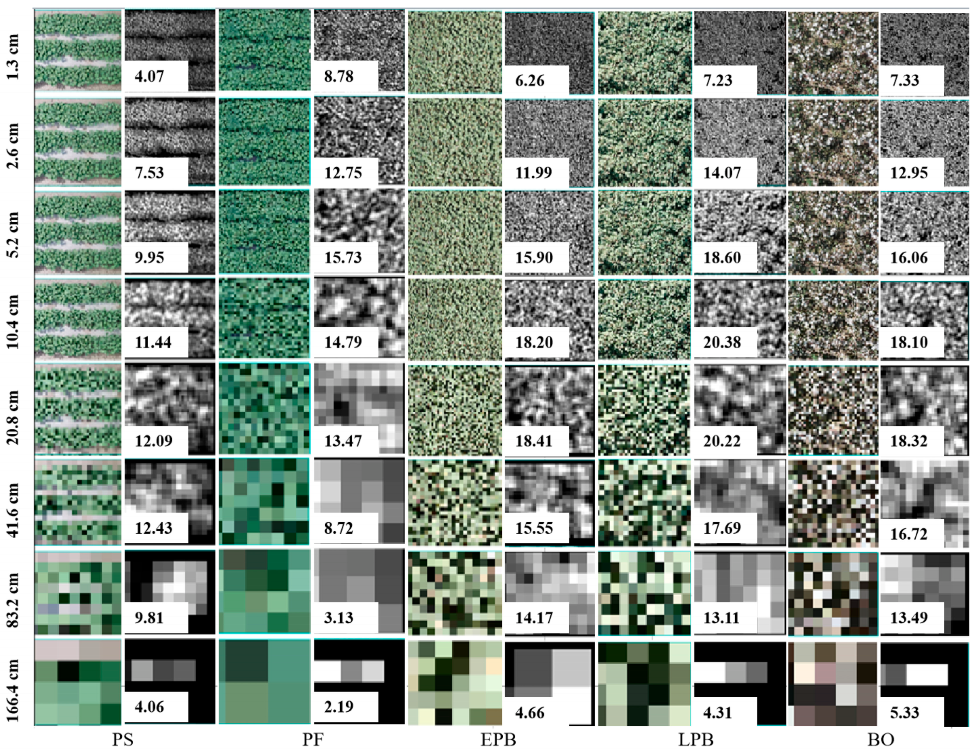
3.3. The Correlation of Image Textures at Different Ground Resolutions of the Image

The Pearson correlation coefficients of the input variables for each channel texture at different ground-resolution images are shown in Figure 6. The results showed that there was a positive correlation between most textures of images with different ground resolutions. Specifically, there was a positive correlation among image textures at 1.3, 2.6, 5.2, 10.4, 20.8, and 41.6 cm ground-resolution images, and the correlation between the texture of the original resolution image and the texture at other resolutions gradually decreases as the resolution decreases, which was most obvious at 41.6 cm. It was shown from another side that the cotton image texture depended on the image’s ground resolution; therefore, while estimating LNC, the image texture needed to be calculated from images with different ground resolutions.

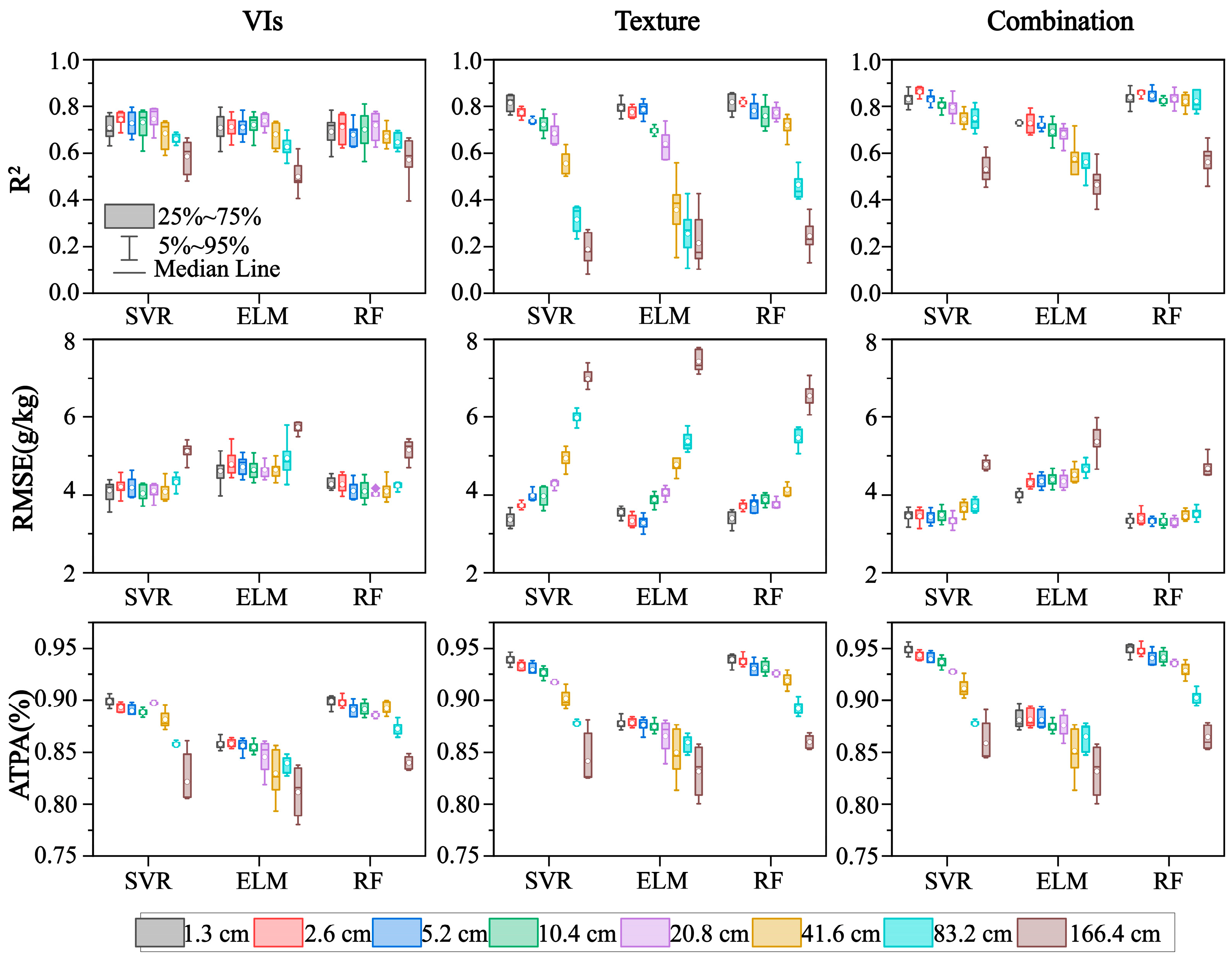
3.4. The Effect of Different Ground-Resolution Images on LNC Estimation by Using RF

Figure 7 shows the performance of eight different ground-resolution images for LNC estimation using only RF. In general, relatively higher ground resolution yielded higher estimation accuracy. Specifically, ground resolutions above 20.8 cm pixel⁻¹ had relatively high estimation accuracy with R² above 0.77, regardless of which metric or regression was used. Secondly, using the same regression method, the accuracy of the combination of VIs and texture was stronger than using VIs or texture alone, while the performance when using texture was stronger than using VIs. The highest accuracy was obtained at 5.2 cm pixel⁻¹ using RF with a combination of VIs and texture. Although the comparable estimation accuracy could also be obtained using a ground resolution of 10.4 cm and 20.8 cm pixel⁻¹, it was still not as stabilized as the ground resolution of 5.2 cm pixel⁻¹ (Figure 8).

3.5. Performance of Three Machine Learning Techniques in LNC Estimation at Different Ground Resolutions

The distributions of R², RMSE, and ATPA for the testing datasets are displayed in Figure 8. The three machine learning techniques yielded similar results to the calibration, with a slightly higher ATPA being observed for the validation datasets. The validation results indicated that RF and SVR regression techniques produced similar R² and RMSE values for LNC estimation. Specifically, the RMSE, R², and ATPA were close at 1.3, 2.6, 5.2, 10.4, 20.8, and 41.6 cm ground-resolution images. However, the R², RMSE, and ATPA changed sharply at a 41.6 cm ground resolution, and R² and ATPA decreased faster (except for VIs). Under combined data, RF with 5.2 cm as the input variable had the highest LNC estimation accuracy, and SVR with 2.6 cm had the highest LNC estimation accuracy. Compared with the SVR models, the RF models had higher accuracy for LNC estimations. The highest ATPA values for LNC estimations were 90.31%, 94.13%, and 95.42%, respectively, in RF models, which were 4.12%, 5.45%, and 5.73% higher than the corresponding optimal ELM models (

Table A2. Validation of three machine learning techniques (MLT) for estimating LNC from various input data types, with RMSE, R², and ATPA results from 100 dataset splits.

Validation	MLT	Input Data Types	Ground Resolutions (cm)
			1.3	2.6	5.2	10.4	20.8	41.6	83.2	166.4
R2	SVR	VIs	0.71	0.75	0.73	0.73	0.75	0.69	0.66	0.59
		Texture	0.82	0.77	0.74	0.72	0.69	0.56	0.32	0.19
		Combination	0.83	0.86	0.83	0.80	0.80	0.75	0.75	0.53
	ELM	VIs	0.71	0.71	0.71	0.72	0.74	0.68	0.63	0.50
		Texture	0.79	0.78	0.79	0.70	0.64	0.36	0.26	0.22
		Combination	0.73	0.73	0.72	0.69	0.68	0.58	0.56	0.46
	RF	VIs	0.69	0.71	0.68	0.70	0.72	0.67	0.65	0.57
		Texture	0.82	0.82	0.78	0.76	0.77	0.72	0.46	0.25
		Combination	0.84	0.86	0.85	0.83	0.83	0.82	0.82	0.56
RMSE	SVR	VIs	4.11	4.21	4.19	4.04	4.11	4.09	4.34	5.13
		Texture	3.38	3.73	3.99	3.97	4.29	4.94	5.98	6.98
		Combination	3.46	3.46	3.44	3.49	3.35	3.65	3.72	4.79
	ELM	VIs	4.62	4.79	4.72	4.65	4.65	4.65	4.95	5.74
		Texture	3.56	3.34	3.29	3.89	4.07	4.78	5.39	7.43
		Combination	4.01	4.31	4.35	4.40	4.36	4.52	4.67	5.38
	RF	VIs	4.28	4.28	4.10	4.09	4.03	4.10	4.25	5.17
		Texture	3.40	3.71	3.76	3.87	3.75	4.14	5.47	6.54
		Combination	3.34	3.41	3.33	3.34	3.30	3.46	3.51	4.68
ATPA	SVR	VIs	0.90	0.89	0.89	0.89	0.90	0.88	0.86	0.82
		Texture	0.94	0.93	0.93	0.93	0.92	0.90	0.88	0.84
		Combination	0.95	0.94	0.94	0.94	0.93	0.91	0.88	0.86
	ELM	VIs	0.86	0.86	0.86	0.85	0.85	0.83	0.84	0.81
		Texture	0.88	0.88	0.88	0.87	0.87	0.85	0.86	0.83
		Combination	0.88	0.88	0.88	0.87	0.88	0.85	0.87	0.83
	RF	VIs	0.90	0.90	0.89	0.89	0.89	0.89	0.87	0.84
		Texture	0.94	0.94	0.93	0.93	0.93	0.92	0.89	0.86
		Combination	0.95	0.95	0.94	0.94	0.94	0.93	0.90	0.87

).

4. Discussion

4.1. The Combination of VIs and Texture Improves the Accuracy of LNC Estimation

For a long time, VIs derived from UAV images have been a widely used method for crop LNC estimation; however, their performance still needs improvement in scenarios where only RGB images are accessible [14]. There are three reasons for the reduced accuracy achieved by utilizing only VIs from RGB images. The first reason is the lack of near-infrared channels, which hinders the ability to detect variations in vegetation vigor. Secondly, there are saturation problems in higher canopy cover conditions [44]. The third reason is the challenge of converting digital number values into reflectance due to the broad spectral ranges of visible channels and imprecise spectral response functions [39]. Moreover, the spectrum information utilized in the vegetation indices was primarily obtained from the uppermost layer of leaves in the cotton canopy, which cannot reflect the information of the middle and lower leaves, especially the leaves in the mid- to late-developing season [25], whereas the texture describes the vertical structure of the canopy [20], which can precisely compensate for the shortcomings caused by VIs.

Research has shown that the accuracy of using textures to estimate N nutrition parameters is better than that using VIs in rice [19]. In this study, eight textures with higher correlation with LNC were chosen to estimate LNC (Figure 4), and the accuracy of the estimated LNC using texture alone was significantly higher than that using VIs alone, regardless of the regression method. These results were similar to those of previous studies, but they only used a simple linear regression method in other crops [18]. The reason why using texture performs better than using VIs may be due to the tonal variation between crop canopy interiors that can be captured by the texture metric.

Moreover, we further found that using the combination of VIs and texture had a significant improvement for LNC estimation than that using VIs or texture alone (Table 5). This may be attributed to the statistical advantage due to the increased number of sources, or the redundancy effect of compensating for noise or defective sources, as well as the superposition of the two advantages. Earlier research has drawn comparable conclusions, but they utilized a combination of vegetation indices and canopy height metrics to estimate wheat biomass [14]. Our results illustrate that the fusion of VIs and texture data could be effective in improving N nutrient monitoring. Further, we also tested the multivariate models of LNC on different datasets, and the validation results were satisfactory (Table 5 and Figure 7). However, the suitability of those models may still need to be enhanced by further testing on a wider range of datasets from different geographic sites.

4.2. Comparison of the Four Regression Methods

Stepwise multiple linear regression (SMLR) has been reported to overestimate the vegetation parameters while quantifying them [45]. In this study, the accuracy of SMLR was equal to that of SVR, which may result from the moderate number of SMLR input variables in this study (no more than 22). This is consistent with the results of Li et al. [26]. However, hundreds or thousands of bands are available in spectral analysis [46], so SMLR may not be able to handle high-dimensional information. On the other hand, machine learning algorithms can handle high-dimensional information with multiple input variables and have been widely used to deal with strong nonlinear relationships between crop biochemical parameters with remotely sensed variables [47]. RF regression has been regarded as one of the popular ensemble learning algorithms that can combine a large number of regression sub-models and does not respond to noise and over-fitting [27].

In this study, the performance of RF for LNC estimation using VIs, texture, or their combination was better than that of SMLR, SVR, and ELM (Figure 5 and Figure 8), which may be due to the insensitivity of RF to noise and over-fitting. The results in our study were similar to those of previous studies in that they found that the performance of using RF was better for SMLR, SVR, and artificial neural networks (ANN) for wheat and maize biomass estimation [26,39]. SVR and ELM are both powerful machine learning regression methods; SVR’s biggest advantage is its ability to train using a small number of samples [28], while ELM requires minimal human intervention and no kernel function, making it an efficient and fast learning algorithm [40]. In our study, the accuracy of SVR was consistently moderate while ELM was the worst, which may be due to the input weights and implied layer thresholds being randomly determined in ELM. The utilization of RF regression was found to be advantageous in achieving high accuracy, as it is a dependable and robust method for handling complex and nonlinear regressions. This assertion has also been supported by previous studies [48,49]. The performance of RF regression still needs to be validated in cotton LNC estimation using datasets from more study areas and cultivars.

4.3. The Optimal Resolution for LNC Estimation

A potential disadvantage of acquiring high-resolution images (with a pixel size of 1.3 cm) is the need to fly the UAV at low altitudes, which can be a significant obstacle to acquiring images efficiently over large areas [14]. To overcome this issue, one solution could be to use cameras with even higher resolutions and fly the UAV at higher altitudes. However, this approach would come at a higher cost and increased weight of the equipment. Instead, relatively lower-resolution images can still generate an acceptable accuracy [20,48]. Our results also confirm that similar accuracy was obtained for ground-resolution images at 2.6, 5.2, 10.4, 20.8, and 41.6 cm pixel⁻¹, with R² above 0.77, compared to a ground resolution of 1.3 cm pixel⁻¹ (Figure 7). This observation is supported by the results of the correlation analysis performed on the texture variables at varying ground resolutions (Figure 6), where the correlation between the image textures at 1.3, 2.6, 5.2, 10.4, 20.8, and 41.6 cm pixel⁻¹ was relatively high. However, the performance of ground resolution at 10.4, 20.8, and 41.6 cm pixel⁻¹ resolutions was not stable (Figure 8). Therefore, it is possible to maintain similar performance between 1.3 and 5.2 cm pixel⁻¹ resolutions by adjusting the flight altitude.

In this study, the optimal resolution estimated was 5.2 cm pixel⁻¹ image resolution for LNC estimation (Figure 7 and Figure 8). When the resolution was reduced to 5.2 cm pixel⁻¹ from the initial resolution of 1.3 cm pixel⁻¹ at 10 m, the shape of the cotton canopy underwent only slight changes but remained discernible with ease (Figure 9). When decreased to a lower resolution, the mixed pixels from the cotton and soil background resulted in the decreased accuracy of LNC estimation. Based on our findings, we suggest utilizing a resolution of 5.2 cm pixel⁻¹ for UAV campaigns. This approach would enable us to enhance the flight efficiency by up to four times with the same UAV without compromising the accuracy of the estimation, leading to significant savings in UAV flight time. Therefore, a relatively low-resolution (5.2 cm pixel⁻¹) image by increasing the flying height or using a lower-resolution camera can still produce an acceptable accuracy.

4.4. The Physiological Basis of VIs and Texture Features in LNC Estimation

In this study, we enhanced the accuracy of estimating LNC by integrating VIs and texture features, further revealing the relationship between these remote sensing indicators and plant physiological activities. VIs are important indicators reflecting the chlorophyll content and photosynthetic efficiency of plant leaves, which are closely related to the nitrogen nutritional status of plants [50]. Typically, sufficient nitrogen nutrition leads to an increase in chlorophyll content, improving photosynthetic efficiency and plants’ water use efficiency. These changes can be monitored through VIs. Conversely, when nitrogen nutrition is insufficient, plants adjust their leaf angles to optimize photosynthesis, and these subtle changes in canopy structure can be captured through texture feature analysis [51]. Therefore, by combining VIs and texture features, we not only improve the accuracy of LNC estimation but also provide new insights into how nitrogen nutritional status affects crops’ physiological responses. This is significant for guiding nitrogen fertilizer management in agricultural production, helping to enhance nitrogen fertilizer efficiency and promote sustainable agricultural development.

5. Conclusions

In this study, we employed a low-cost (UAV system to capture RGB imagery under varying nitrogen fertilizer treatments (195.5, 299, 402.5, and 506 kg N ha⁻¹) and seeding densities (6.9 × 10⁴, 13.8 × 10⁴, and 24 × 10⁴ plants ha⁻¹), with the aim of accurately assessing the nitrogen status of drip-irrigated cotton. We evaluated the effectiveness of image texture and VIs at different ground resolutions (1.3 to 166.4 cm) for estimating LNC in cotton, applying four regression methods (SMLR, SVR, ELM, RF). The results demonstrated that the combination of VIs (ExGR, GRVI, GBRI, GRRI, MGRVI, RGBVI) and texture features (VAR, HOM, CON, DIS) enhanced the accuracy of LNC estimation, particularly when employing the RF regression model. This model performed exceptionally well at high resolution (1.3 cm) and maintained good estimation accuracy even at lower resolutions (5.2 cm). Therefore, the use of RF algorithms to combine VIs and texture information obtained from inexpensive UAV systems may have potential value in the rapid estimation of other parameters in practical applications. Future research could further explore the applicability of these techniques across different crops and environmental conditions, and optimize algorithms and image-processing techniques to enhance their practicality and prevalence in real-world agricultural management. We also acknowledge the role of organic residues in soil fertility and nitrogen management as an important area of research. Although not a part of our current study, this indeed represents a direction worth considering for future work.

References

1. Hou, Z.N.; Li, P.F.; Li, B.G.; Gong, J.; Wang, Y.N. Effects of fertigation scheme on N uptake and N use efficiency in cotton. Plant Soil 2007, 290, 115–126. [Google Scholar] [CrossRef]
2. Ata-Ul-Karim, S.T.; Zhu, Y.; Cao, Q.; Rehmani, M.I.A.; Cao, W.X.; Tang, L. In-season assessment of grain protein and amylose content in rice using critical nitrogen dilution curve. Eur. J. Agron. 2017, 90, 139–151. [Google Scholar] [CrossRef]
3. Bodirsky, B.L.; Popp, A.; Lotze-Campen, H.; Dietrich, J.P.; Rolinski, S.; Weindl, I.; Schmitz, C.; Muller, C.; Bonsch, M.; Humpenoder, F.; et al. Reactive nitrogen requirements to feed the world in 2050 and potential to mitigate nitrogen pollution. Nat. Commun. 2014, 5, 38–58. [Google Scholar] [CrossRef] [PubMed]
4. Yao, X.; Zhu, Y.; Tian, Y.C.; Feng, W.; Cao, W.X. Exploring hyperspectral bands and estimation indices for leaf nitrogen accumulation in wheat. Int. J. Appl. Earth Obs. Geoinf. 2010, 12, 89–100. [Google Scholar] [CrossRef]
5. Li, S.Y.; Ding, X.Z.; Kuang, Q.L.; Ata-Ul-Karim, S.T.; Cheng, T.; Liu, X.J.; Tan, Y.C.; Zhu, Y.; Cao, W.X.; Cao, Q. Potential of UAV-Based Active Sensing for Monitoring Rice Leaf Nitrogen Status. Front. Plant Sci. 2018, 9, 1834. [Google Scholar] [CrossRef] [PubMed]
6. LaCapra, V.C.; Melack, J.M.; Gastil, M.; Valeriano, D. Remote sensing of foliar chemistry of inundated rice with imaging spectrometry. Remote Sens. Environ. 1996, 55, 50–58. [Google Scholar] [CrossRef]
7. Blaes, X.; Chome, G.; Lambert, M.J.; Traore, P.S.; Schut, A.G.T.; Defourny, P. Quantifying Fertilizer Application Response Variability with VHR Satellite NDVI Time Series in a Rainfed Smallholder Cropping System of Mali. Remote Sens. 2016, 8, 531. [Google Scholar] [CrossRef]
8. Boegh, E.; Soegaard, H.; Broge, N.; Hasager, C.B.; Jensen, N.O.; Schelde, K.; Thomsen, A. Airborne multispectral data for quantifying leaf area index, nitrogen concentration, and photosynthetic efficiency in agriculture. Remote Sens. Environ. 2002, 81, 179–193. [Google Scholar] [CrossRef]
9. Tilling, A.K.; O’Leary, G.J.; Ferwerda, J.G.; Jones, S.D.; Fitzgerald, G.J.; Rodriguez, D.; Belford, R. Remote sensing of nitrogen and water stress in wheat. Field Crops Res. 2007, 104, 77–85. [Google Scholar] [CrossRef]
10. Yao, X.; Ren, H.; Cao, Z.; Tian, Y.; Cao, W.; Zhu, Y.; Cheng, T. Detecting leaf nitrogen content in wheat with canopy hyperspectrum under different soil backgrounds. Int. J. Appl. Earth Obs. Geoinf. 2014, 32, 114–124. [Google Scholar] [CrossRef]
11. Schut, A.G.T.; Traore, P.C.S.; Blaes, X.; de By, R.A. Assessing yield and fertilizer response in heterogeneous smallholder fields with UAVs and satellites. Field Crops Res. 2018, 221, 98–107. [Google Scholar] [CrossRef]
12. Amaral, L.R.; Molin, J.P.; Portz, G.; Finazzi, F.B.; Cortinove, L. Comparison of crop canopy reflectance sensors used to identify sugarcane biomass and nitrogen status. Precis. Agric. 2015, 16, 15–28. [Google Scholar] [CrossRef]
13. Jiang, J.L.; Cai, W.D.; Zheng, H.B.; Cheng, T.; Tian, Y.C.; Zhu, Y.; Ehsani, R.; Hu, Y.Q.; Niu, Q.S.; Gui, L.J.; et al. Using Digital Cameras on an Unmanned Aerial Vehicle to Derive Optimum Color Vegetation Indices for Leaf Nitrogen Concentration Monitoring in Winter Wheat. Remote Sens. 2019, 11, 2667. [Google Scholar] [CrossRef]
14. Lu, N.; Zhou, J.; Han, Z.X.; Li, D.; Cao, Q.; Yao, X.; Tian, Y.C.; Zhu, Y.; Cao, W.X.; Cheng, T. Improved estimation of aboveground biomass in wheat from RGB imagery and point cloud data acquired with a low-cost unmanned aerial vehicle system. Plant Methods 2019, 15, 17. [Google Scholar] [CrossRef] [PubMed]
15. Prey, L.; Schmidhalter, U. Sensitivity of Vegetation Indices for Estimating Vegetative N Status in Winter Wheat. Sensors 2019, 19, 3712. [Google Scholar] [CrossRef] [PubMed]
16. Zhou, K.; Cheng, T.; Zhu, Y.; Cao, W.X.; Ustin, S.L.; Zheng, H.B.; Yao, X.; Tian, Y.C. Assessing the Impact of Spatial Resolution on the Estimation of Leaf Nitrogen Concentration Over the Full Season of Paddy Rice Using Near-Surface Imaging Spectroscopy Data. Front. Plant Sci. 2018, 9, 964. [Google Scholar] [CrossRef]
17. Zhao, B.; Ata-Ul-Karim, S.T.; Yao, X.; Tian, Y.C.; Cao, W.X.; Zhu, Y.; Liu, X.J. A New Curve of Critical Nitrogen Concentration Based on Spike Dry Matter for Winter Wheat in Eastern China. PLoS ONE 2016, 11, e0164545. [Google Scholar] [CrossRef]
18. Yue, J.B.; Yang, G.J.; Tian, Q.J.; Feng, H.K.; Xu, K.J.; Zhou, C.Q. Estimate of winter-wheat above-ground biomass based on UAV ultrahigh-ground-resolution image textures and vegetation indices. ISPRS J. Photogramm. Remote Sens. 2019, 150, 226–244. [Google Scholar] [CrossRef]
19. Zheng, H.B.; Ma, J.F.; Zhou, M.; Li, D.; Yao, X.; Cao, W.X.; Zhu, Y.; Cheng, T. Enhancing the Nitrogen Signals of Rice Canopies across Critical Growth Stages through the Integration of Textural and Spectral Information from Unmanned Aerial Vehicle (UAV) Multispectral Imagery. Remote Sens. 2020, 12, 957. [Google Scholar] [CrossRef]
20. Zhang, X.W.; Zhang, K.F.; Wu, S.Q.; Shi, H.T.; Sun, Y.Q.; Zhao, Y.D.; Fu, E.J.; Chen, S.; Bian, C.F.; Ban, W. An Investigation of Winter Wheat Leaf Area Index Fitting Model Using Spectral and Canopy Height Model Data from Unmanned Aerial Vehicle Imagery. Remote Sens. 2022, 14, 5087. [Google Scholar] [CrossRef]
21. Xu, C.; Ding, Y.L.; Zheng, X.M.; Wang, Y.Q.; Zhang, R.; Zhang, H.Y.; Dai, Z.W.; Xie, Q.Y. A Comprehensive Comparison of Machine Learning and Feature Selection Methods for Maize Biomass Estimation Using Sentinel-1 SAR, Sentinel-2 Vegetation Indices, and Biophysical Variables. Remote Sens. 2022, 14, 4083. [Google Scholar] [CrossRef]
22. Zheng, H.B.; Cheng, T.; Zhou, M.; Li, D.; Yao, X.; Tian, Y.C.; Cao, W.X.; Zhu, Y. Improved estimation of rice aboveground biomass combining textural and spectral analysis of UAV imagery. Precis. Agric. 2019, 20, 611–629. [Google Scholar] [CrossRef]
23. Singh, B.; Singh, Y.; Ladha, J.K.; Bronson, K.F.; Balasubramanian, V.; Singh, J.; Khind, C.S. Chlorophyll meter- and leaf color chart-based nitrogen management for rice and wheat in northwestern India. Agron. J. 2002, 94, 821–829. [Google Scholar] [CrossRef]
24. Niu, Y.X.; Zhang, L.Y.; Zhang, H.H.; Han, W.T.; Peng, X.S. Estimating Above-Ground Biomass of Maize Using Features Derived from UAV-Based RGB Imagery. Remote Sens. 2019, 11, 1261. [Google Scholar] [CrossRef]
25. Ma, Y.R.; Ma, L.L.; Zhang, Q.; Huang, C.P.; Yi, X.; Chen, X.Y.; Hou, T.Y.; Lv, X.; Zhang, Z. Cotton Yield Estimation Based on Vegetation Indices and Texture Features Derived from RGB Image. Front. Plant Sci. 2022, 13, 925986. [Google Scholar] [CrossRef]
26. Li, W.; Niu, Z.; Chen, H.Y.; Li, D.; Wu, M.Q.; Zhao, W. Remote estimation of canopy height and aboveground biomass of maize using high-resolution stereo images from a low-cost unmanned aerial vehicle system. Ecol. Indic. 2016, 67, 637–648. [Google Scholar] [CrossRef]
27. Breiman, L. Random forests. Mach. Learn. 2001, 45, 5–32. [Google Scholar] [CrossRef]
28. Mountrakis, G.; Im, J.; Ogole, C. Support vector machines in remote sensing: A review. ISPRS J. Photogramm. Remote Sens. 2011, 66, 247–259. [Google Scholar] [CrossRef]
29. Huang, G.B.; Zhu, Q.Y.; Siew, C.K. Extreme learning machine: Theory and applications. Neurocomputing 2006, 70, 489–501. [Google Scholar] [CrossRef]
30. Bremner, J.M. Recent research on problems in the use of urea as a nitrogen fertilizer. Fertil. Res. 1995, 42, 321–329. [Google Scholar] [CrossRef]
31. Haralick, R.M.; Sabaretnam, K. Textural features for image classification. IEEE Trans. Syst. Man Cybern. 1973, SMC-3, 610–621. [Google Scholar] [CrossRef]
32. Kawashima, S.; Nakatani, M. An algorithm for estimating chlorophyll content in leaves using a video camera. Ann. Bot. 1998, 81, 49–54. [Google Scholar] [CrossRef]
33. Louhaichi, M.; Borman, M.M.; Johnson, D.E. Spatially Located Platform and Aerial Photography for Documentation of Grazing Impacts on Wheat. Geocarto Int. 2001, 16, 65–70. [Google Scholar] [CrossRef]
34. Meyer, G.E.; Neto, J.C. Verification of color vegetation indices for automated crop imaging applications. Comput. Electron. Agric. 2008, 63, 282–293. [Google Scholar] [CrossRef]
35. Johnson, D.E.; Harris, N.R.; Louhaichi, M.; Casady, G.M.; Borman, M.M. Mapping selected noxious weeds using remote sensing and geographic information systems. Abstr. Pap. Am. Chem. Soc. 2001, 221, 48. [Google Scholar]
36. Woebbecke, D.M.; Meyer, G.E.; Vonbargen, K.; Mortensen, D.A. Color Indexes for Weed Identification under Various Soil, Residue, and Lighting Conditions. Trans. ASAE 1995, 38, 259–269. [Google Scholar] [CrossRef]
37. Gitelson, A.A.; Kaufman, Y.J.; Stark, R.; Rundquist, D. Novel algorithms for remote estimation of vegetation fraction. Remote Sens. Environ. 2002, 80, 76–87. [Google Scholar] [CrossRef]
38. Zheng, H.; Cheng, T.; Li, D.; Zhou, X.; Yao, X.; Tian, Y.; Cao, W.; Zhu, Y. Evaluation of RGB, Color-Infrared and Multispectral Images Acquired from Unmanned Aerial Systems for the Estimation of Nitrogen Accumulation in Rice. Remote Sens. 2018, 10, 824. [Google Scholar] [CrossRef]
39. Mutanga, O.; Adam, E.; Cho, M.A. High density biomass estimation for wetland vegetation using WorldView-2 imagery and random forest regression algorithm. Int. J. Appl. Earth Obs. Geoinf. 2012, 18, 399–406. [Google Scholar] [CrossRef]
40. Huang, G.B.; Zhou, H.M.; Ding, X.J.; Zhang, R. Extreme Learning Machine for Regression and Multiclass Classification. IEEE Trans. Syst. Man Cybern. Part B-Cybern. 2012, 42, 513–529. [Google Scholar] [CrossRef]
41. Cortes, C.; Vapnik, V. Support-Vector Networks. Mach. Learn. 1995, 20, 273–297. [Google Scholar] [CrossRef]
42. Gao, Y.K.; Lu, D.S.; Li, G.Y.; Wang, G.X.; Chen, Q.; Liu, L.J.; Li, D.Q. Comparative Analysis of Modeling Algorithms for Forest Aboveground Biomass Estimation in a Subtropical Region. Remote Sens. 2018, 10, 627. [Google Scholar] [CrossRef]
43. Lin, L.; Wang, F.; Xie, X.L.; Zhong, S.S. Random forests-based extreme learning machine ensemble for multi-regime time series prediction. Expert Syst. Appl. 2017, 83, 164–176. [Google Scholar] [CrossRef]
44. Jin, X.L.; Yang, G.J.; Xu, X.G.; Yang, H.; Feng, H.K.; Li, Z.H.; Shen, J.X.; Zhao, C.J.; Lan, Y.B. Combined Multi-Temporal Optical and Radar Parameters for Estimating LAI and Biomass in Winter Wheat Using HJ and RADARSAR-2 Data. Remote Sens. 2015, 7, 13251–13272. [Google Scholar] [CrossRef]
45. Grossman, Y.L.; Ustin, S.L.; Jacquemoud, S.; Sanderson, E.W.; Schmuck, G.; Verdebout, J. Critique of stepwise multiple linear regression for the extraction of leaf biochemistry information from leaf reflectance data. Remote Sens. Environ. 1996, 56, 182–193. [Google Scholar] [CrossRef]
46. Jia, F.F.; Liu, G.S.; Liu, D.S.; Zhang, Y.Y.; Fan, W.G.; Xing, X.X. Comparison of different methods for estimating nitrogen concentration in flue-cured tobacco leaves based on hyperspectral reflectance. Field Crops Res. 2013, 150, 108–114. [Google Scholar] [CrossRef]
47. Gleason, C.J.; Im, J. Forest biomass estimation from airborne LiDAR data using machine learning approaches. Remote Sens. Environ. 2012, 125, 80–91. [Google Scholar] [CrossRef]
48. Wang, L.A.; Zhou, X.D.; Zhu, X.K.; Dong, Z.D.; Guo, W.S. Estimation of biomass in wheat using random forest regression algorithm and remote sensing data. Crop J. 2016, 4, 212–219. [Google Scholar] [CrossRef]
49. Zarco-Tejada, P.J.; Diaz-Varela, R.; Angileri, V.; Loudjani, P. Tree height quantification using very high resolution imagery acquired from an unmanned aerial vehicle (UAV) and automatic 3D photo-reconstruction methods. Eur. J. Agron. 2014, 55, 89–99. [Google Scholar] [CrossRef]
50. Nasar, J.; Wang, G.Y.; Ahmad, S.; Muhammad, I.; Zeeshan, M.; Gitari, H.; Adnan, M.; Fahad, S.; Khalid, M.H.B.; Zhou, X.B.; et al. Nitrogen fertilization coupled with iron foliar application improves the photosynthetic characteristics, photosynthetic nitrogen use efficiency, and the related enzymes of maize crops under different planting patterns. Front. Plant Sci. 2022, 13, 988055. [Google Scholar] [CrossRef]
51. Zheng, J.C.; Zhang, H.; Yu, J.; Zhan, Q.W.; Li, W.Y.; Xu, F.; Wang, G.J.; Liu, T.; Li, J.C. Late Sowing and Nitrogen Application to Optimize Canopy Structure and Grain Yield of Bread Wheat in a Fluctuating Climate. Turk. J. Field Crops 2021, 26, 170–179. [Google Scholar] [CrossRef]
Figure 1. Location of the experimental site and layout of the field plots (a,b). The orthophoto was captured with the UAV system at the full bud stage of cotton on 30 June 2019 (c). Note: GCP ground control point, SP sampling area; N1 = 195.5, N2 = 299, N3 = 402.5, N4 = 506 kg N ha−1.
Agronomy 14 00120 g001
Figure 2. Diagram of three density planting patterns for field trials. Note: These three planting patterns are widely used in local cotton production.
Agronomy 14 00120 g002
Figure 3. The changes of digital number values in different channels with LNC (a) and Pearson’s correlation coefficients (r) between LNC and individual UAV-derived vegetation indices (b).
Agronomy 14 00120 g003
Figure 4. The Pearson correlation coefficient between the different bands of the texture and LNC. Note: PS: full bud stage; PF: full flowering stage; EPB: early full-bolling stage; LPB: late full-bolling stage; BO: boll opening stage; All: the whole growth stage.
Agronomy 14 00120 g004
Figure 5. Scatterplots of measured LNC (g kg−1) in cotton and LNC estimated with three machine learning techniques (left: SMLR, second column: SVR, third column: ELM, right: RF) from the VIs alone (ad), texture alone (eh), and the combined data (il). The data points displayed in each plot represent the validation set. The dashed diagonals represent 1:1 line and the solid lines represent the fitted linear function.
Agronomy 14 00120 g005
Figure 6. Pearson’s correlation coefficient between input variables of the texture in different ground-resolution images. Note: GR for the different ground resolutions; for example, GR1.3 represents textures from images with 1.3 cm ground resolution. R-, G-, and B- represent the textures corresponding to the three bands of RGB, respectively; for example, R-Variance represents the texture of Variance from the R-band.
Agronomy 14 00120 g006
Figure 7. The performance of LNC estimation from three types of input data. Note: top rows: VIs; middle rows: texture; bottom rows: the combination of VIs and texture) for a series of pixel sizes using the RF technique.
Agronomy 14 00120 g007
Figure 8. Validation of three machine learning techniques for estimating LNC from various input data types (left column: VIs; middle column: texture; right column: combination of VIs and texture), with RMSE, R2, and ATPA results from 100 dataset splits.
Agronomy 14 00120 g008
Figure 9. RGB image and corresponding B-band DIS and values. Note: PS: full bud stage; PF: full flowering stage; EPB: early full-bolling stage; LPB: late full-bolling stage; BO: boll opening stage; All: the whole growth stage.
Agronomy 14 00120 g009