Detection and Analysis of Chili Pepper Root Rot by Hyperspectral Imaging Technology

Abstract

The objective is to develop a portable device capable of promptly identifying root rot in the field. This study employs hyperspectral imaging technology to detect root rot by analyzing spectral variations in chili pepper leaves during times of health, incubation, and disease under the stress of root rot. Two types of chili pepper seeds (Manshanhong and Shanjiao No. 4) were cultured until they had grown two to three pairs of true leaves. Subsequently, robust young plants were infected with Fusarium root rot fungi by the root-irrigation technique. The effective wavelength for discriminating between distinct stages was determined using the successive projections algorithm (SPA) after capturing hyperspectral images. The optimal index related to root rot between each normalized difference spectral index (NDSI) was obtained using the Pearson correlation coefficient. The early detection of root rot illness can be modeled using spectral information at effective wavelengths and in NDSI, together with the application of partial least squares discriminant analysis (PLS-DA), least squares support vector machine (LSSVM), and back-propagation (BP) neural network technology. The SPA-BP model demonstrates outstanding predictive capabilities compared with other models, with a classification accuracy of 92.3% for the prediction set. However, employing SPA to acquire an excessive number of efficient wave-lengths is not advantageous for immediate detection in practical field scenarios. In contrast, the NDSI (R₄₄₅, R₄₃₃)-BP model uses only two wavelengths of spectral information, but the prediction accuracy can reach 89.7%, which is more suitable for rapid detection of root rot. This thesis can provide theoretical support for the early detection of chili root rot and technical support for the design of a portable root rot detector.

1. Introduction

The chili pepper (Capsicum) is a vegetable category with the most comprehensive industrial chain in China, boasting a cultivation history of over 400 years. Its ability to produce capsaicin, which provides it its spicy taste, and its high vitamin C content make it the leading vegetable in China’s flavoring varieties, thus holding a significant position. The root rot of chili pepper has been steadily increasing in various regions due to the fixed cultivation mode, large continuous cropping area, extensive management, and weak ability to resist drought and flood disasters. This has led to reduced or no production of chili pepper, severely hampering the development of the chili pepper industry and causing significant economic losses for farmers. Chili pepper root rot is a common disease caused by soil-borne pathogens. It leads to the death of chili pepper roots and the vascular tissues (xylem and phloem) in the lower stems, which hinders the plant’s capacity to transfer water and nutrients. Following the onset of the disease, the subterranean portion’s roots and stems exhibit complete necrosis, while the aerial portion appears desiccated and lifeless [1]. The disease is prevalent in all regions of China where chili peppers are cultivated. The early stage of chili pepper root rot is characterized by its remarkable ability to conceal itself, making it challenging to detect with the human eye. To control soil-borne diseases, such as chili pepper root rot, it is generally recommended to regularly monitor the distribution of pathogenic pathogens in the soil, control their density, and prevent their spread through the use of biological and chemical control agents. Among them, regular inspections demand significant time from plant health inspectors and necessitate a high level of professional expertise [2,3,4]. Hence, there is a pressing requirement for chili pepper cultivators to devise a novel technique capable of identifying chili pepper root rot by examining the visible portions (leaves or stems) of the plants, even in the absence of symptoms.

In recent years, machine vision systems based on visible light images have been widely used in fruit and vegetable disease detection [5]. When using machine vision to detect fruits and vegetables, machine learning algorithms and deep learning models are usually used to identify diseases and detect whether crops have been infected based on the special characteristics of crop leaves [6]. For example, T. Daniya et al. designed a rice disease detection method using a neural network based on Rider water waves (RWW-NN). This network uses RWW, which is a fusion of Rider optimization algorithm (ROA) and water wave optimization algorithm (WWO), to complete neural network training, and the highest recognition accuracy can reach 0.908 [7]. Asif Iqbal Khan et al. constructed a suitable-sized apple disease dataset consisting of about 9000 high-quality RGB images, covering all major leaf diseases and symptoms. After that, based on this data set, an Apple disease detection system based on deep learning models such as EfficientDet, Yolov4, and Fast-RCNN is proposed. The classification accuracy can reach about 88% in a higher detection rate [8]. However, the use of machine vision to detect plant diseases is essentially done when the plant is already characterized by the disease. The disease manifestation of the plant must exhibit clear visual distinctions from a healthy individual, serving as the primary prerequisite for employing machine vision in the detection of plant illnesses.

Due to the constraints of machine vision, hyperspectral imaging is increasingly being preferred for plant disease identification. Allen Benjamin et al. used drones to collect hyperspectral images and detected the root rot of Norwegian spruce at two sites in Norway. The support vector machine (SVM) algorithm was used to classify healthy and root rot-infected Norway spruce, and the classification accuracy of hyperspectral images at 490 bands was as high as 76% [9]. Adam Elhadi et al. study aimed to investigate the use of hyperspectral data to detect the early stages of brown spot disease (BSD) in tropical maize. Spectral data were collected from healthy and early stages of BSD (2013 and 2014) maize leaves, and feature selection and classification were performed using bootstrap regularized random forest (BRRF) and traditional random forest (RF), which showed that there were statistically significant differences in biochemical concentrations between healthy leaves and leaves in the early stages of BSD infestation and that the random forest classifier was able to stage to distinguish between healthy and infested maize with an overall accuracy of 88% [10]. Wenjing Ba et al. used micro-near infrared spectroscopy to detect early wheat blast infection, and combined SG+SNV with Autogluon (with SVM) model to obtain the optimal classification results with an accuracy of 73.33% [11]. CHEN Bing et al. used canopy spectral data of cotton flowers in Xinjiang in 2005–2006 and yellow blight Using the 2005–2006 canopy spectral data of Xinjiang cotton and the severity data of yellow wilt disease, the incidence pattern of yellow wilt disease in Xinjiang cotton was studied. It was found that the canopy spectral characteristics of cotton yellow wilt in different periods and varieties changed regularly with the intensity of disease-sensitive light. Their study found that FD_{731 nm}–FD_{1317 nm} based on first-order derivative spectra was the best identification and could be used for quantitative prediction of yellow wilt infection in cotton canopies [12]. It is worth mentioning that the spectral index is a commonly used data dimension reduction method in hyperspectral imaging technology. The spectral index is a quantitative measure obtained by comparing the reflectance or absorption rates of two or three distinct bands. The spectral index only uses the spectral information of two or three different bands in the hyperspectral image, which greatly reduces the analysis of redundant data. Abdulridha Jaafar et al. calculated 408 spectral vegetation indices (VIs) to select the best index for improving the detection and recognition accuracy of tomato diseases. Two classification methods were used: multi-layer perceptron (MLP) neural network and stepwise discriminant analysis (STDA). The best band selection was considered to be blue (420–630 nm), red (650–700 nm) and red edge (710–730 nm). The classification results between healthy plants and diseased plants have high accuracy for all diseases; for example, the classification rates of healthy and bacterial spots (BS), asymptomatic target spots (TS), and tomato yellow leaf curl (TYLC) were 94%, 95%, and 100%, respectively, under asymptomatic and laboratory conditions [13]. Calamita Federico et al. utilized the hyperspectral imaging sensor Specim IQ to obtain reflectance data of Teroldego Rotaliano wine leaves. The study involved the analysis of three distinct categories of grape plants: the group exhibiting good health, the group showing no symptoms, and the group displaying signs of disease. Notable disparities were seen in the near-infrared (NIR) spectral band. By integrating the Naïve Bayes (NB) algorithm with the most distinguishing variables in the vegetation index and spectral narrowband, the optimal outcomes were achieved, yielding an overall accuracy of 90% for the healthy group and 75% for both the diseased group and the asymptomatic group [14]. Because narrow-band filters and narrow-band light sources are expensive, reducing the number of bands reduces the development costs of portable instruments and makes them more likely to be rolled out in the field. The research above demonstrates the feasibility of using hyperspectral imaging technology to detect fruit and vegetable diseases early. However, there are limited reports on the early detection of chili pepper diseases using hyperspectral imaging technology, particularly for root rot.

The purpose of this study is to explore the potential of hyperspectral imaging technology in the early diagnosis of chili pepper root rot. To this end, the specific objectives are (i) to analyze the spectral reflectance changes in chili pepper leaves at different infection stages and the embodiment of root rot in chili pepper leaves; (ii) Obtaining effective wavelength and NDSI associated with root rot of chili; (iii) Using a variety of algorithms to establish early diagnosis models of root rot disease and evaluate their diagnostic potential.

2. Materials and Methods

2.1. Plant Cultivation and Pathogen Inoculation

The sample preparation was carried out in the laboratory of the Academy of Agricultural Sciences (Jining, China) in September 2023. For the purpose of this experiment, two chili pepper cultivars, namely Manshanhong and Shanjiao No. 4, were chosen for the growing of seedlings. The procedure of cultivating chili pepper seedlings is as follows: The beaker was filled with warm water at a temperature of 55 °C, and the glass rod was swirled constantly for a duration of 10 min. Empty the warm water from the beaker, rinse the seeds two times, and then soak them for a period of 8 to 10 h. Next, arrange the seeds evenly on a damp towel, ensuring that the towel remains moist. Place the towel in a tray and position the tray under a well-lit incubator to facilitate germination, which typically takes around four days. Once the seeds have sprouted, transfer them to seedling cups filled with a mixture of perlite, carbendazim, and organic nutrient soil. Cultivate the seedlings in a well-lit incubator for a duration of 17 days. There was a survival rate of one to three plants per seedling cup. The light incubator was configured with the following conditions: the bright light environment had a culture time of 10 h, a temperature of 28 °C, a humidity of 60%, and a light intensity ranging from 4500 to 10,000 Lux. The dark environment had a culture time of 14 h, a temperature of 23 °C, and a humidity of 60%.

The chili pepper seedlings were infected with the pathogen of root rot by artificial inoculation, and the inoculation steps met the agricultural industry standard of the People’s Republic of China (NY/T 2060.1-2011; Rules for evaluation of pepper for resistance to diseases. Part 1: Rule for evaluation of pepper for resistance to phytophthora. Institute of Vegetable and Flower Research, Chinese Academy of Agricultural Sciences: Beijing, China, 2011). The stock solution of the root rot pathogen used in the experiment was cultured and provided by the Jining Academy of Agricultural Sciences, and the root rot pathogen was inoculated by root irrigation inoculation method. The specific method is: 20 healthy chili pepper seedlings with consistent growth were selected from the two varieties for pathogen inoculation; before inoculation, the seedlings were watered to keep the soil moist, and a small hole was set up near the base of the stem of the chili pepper seedlings by using a glass rod. A 5 mL spore suspension (concentration of 103 zoospores/mL) was injected into the hole using a pipette. After inoculation, the chili pepper seedlings were put back into the light incubator, and the light environment culture time was changed to 12 h, the dark environment culture time was 12 h, and other conditions remained unchanged.

Throughout the experiment, the chili pepper seedlings that were deliberately exposed to pathogens exhibited signs of disease. The chili pepper leaf samples were categorized into three stages: the healthy period (0 d), which refers to the time before inoculation; the incubation period (1 d), which corresponds to the first day of inoculation; and the diseased period (2 d), which represents the second day of inoculation.

2.2. Hyperspectral Imaging System and Image Acquisition

2.2.1. Hyperspectral Imaging System

This experiment used the GaiaField-V10E portable imaging system (Jiangsu Dualix Spectral Imaging Technology Co., Ltd., Wuxi, China) to obtain hyperspectral image information. The system includes a spectrometer (GaiaField-V10E), an imaging lens (HSIA-OL23), a dedicated light source (HSIA-LS-T-200 W), and a standard whiteboard (HSIA-CT-150 × 150) and a dedicated computer (Surface Go 2 4425Y, Microsoft, Washington, USA) installed with the software of SpecView v1.0. for data collection. The device can image in the range of visible and near-infrared bands. The wavelength coverage range is 400–1000 nm, the spectral resolution is 2.8 nm, and each sample can obtain a hyperspectral image cube of 696 × 697 × 256 bands. The exposure time is set to 12 milliseconds, the incident slit width is 30 microns, the field of view is 22°, and the CCD pixel is 1392 × 1040.

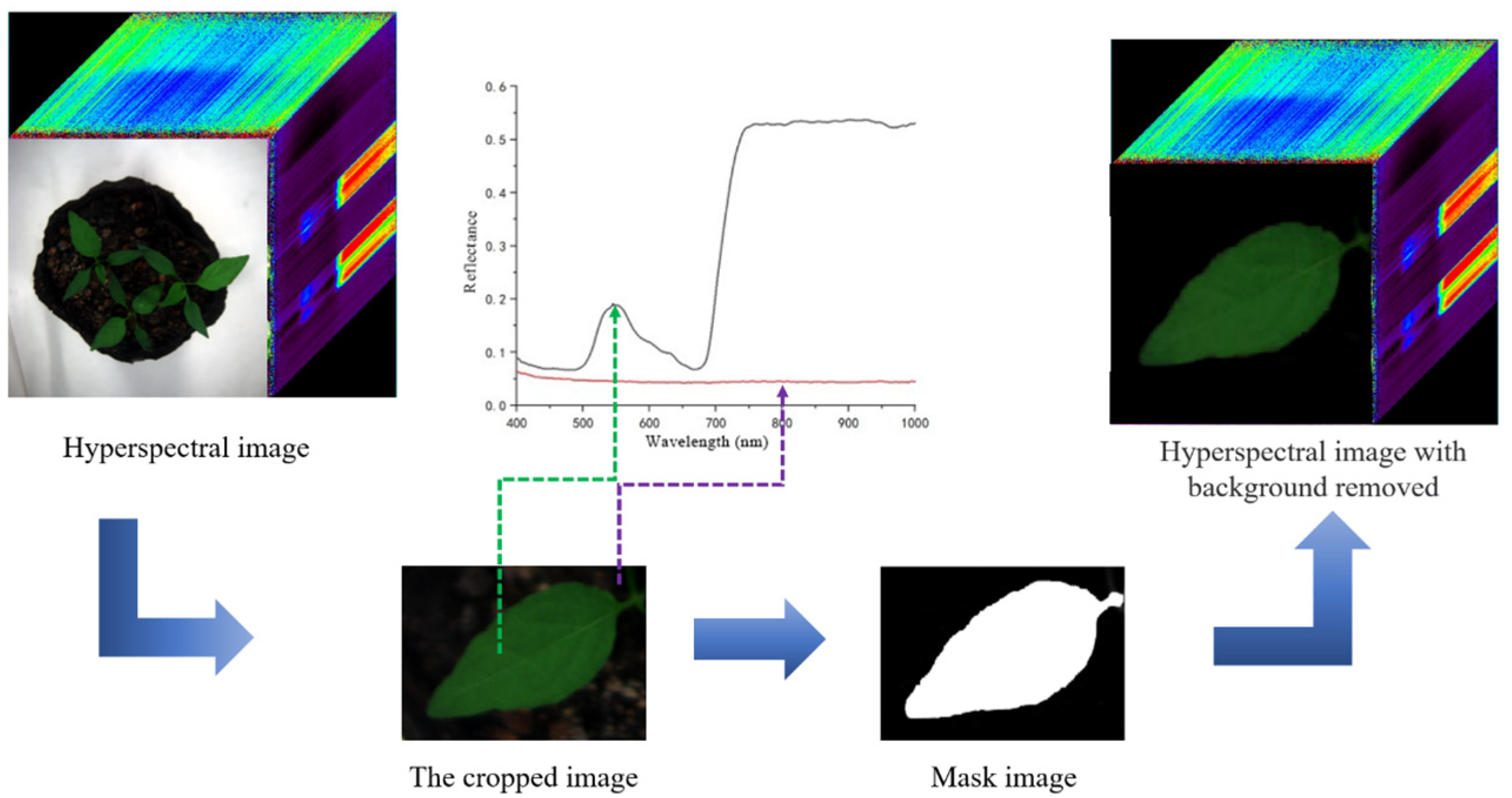
2.2.2. Hyperspectral Image Acquisition and Processing

Hyperspectral images of the chili pepper seedling canopy were collected using a GaiaField-V10E portable hyperspectral instrument appropriately fixed at 40 cm above the plant by means of a tripod. The noise sources of hyperspectral images are complex, and black-and-white correction is one of the important steps to eliminate noise. To achieve black-and-white correction, it is necessary to obtain black reference and white reference. Among them, the white reference is obtained by using white polyethylene (Dualix Instruments Co., Ltd., Chengdu, China) as a reflector, which can reflect almost 99% of the incident light in the visible near-infrared range; the hyperspectral image after the camera lens cover is collected as a dark reference. After black-and-white correction and dark reference processing, the collected images can be used to estimate and eliminate noise using the following mathematical equations to improve the quality and accuracy of spectral images.

$$I_0=\frac{I_{raw}-I_{dark}}{I_{white}-{ I}_{dark}}$$

(1)

where I₀ is the processed hyperspectral image, I_raw is the initial hyperspectral image, I_white is the white reference image, and I_dark is the black reference image.

This paper utilizes MATLAB 2018b (The MathWorks, Natick, MA, USA) to effectively extract the spectrum data of a single chili pepper leaf. The process involves selecting and isolating a single leaf, and then extracting the hyperspectral data using threshold segmentation technology, with the leaf serving as the region of interest (ROI). Figure 1 illustrates the sequence of steps involved in the processing of the mask. The background pixels in the image exhibit minimal variation in reflectivity throughout the entire region. However, the reflectivity of the sample undergoes a substantial range of change between 400 and 680 nm, while the change is minimal between 800 and 880 nm. Furthermore, there is a notable disparity between the reflectivity of the sample and the background reflectivity. Thus, by employing threshold segmentation technology on hyperspectral pictures with a wavelength of 810 nm, a binary image is generated. This image has a background area assigned a value of 0 and a sample area assigned a value of 1. This binary image serves as a mask. A reflectance threshold of 0.2 was established, and the spectral reflectance data of the leaf interest region was retrieved using this mask.

2.3. Dataset Partitioning

To ensure the performance of the model, the sample set partitioning based on the joint X-Y distance (SPXY) algorithm is used to divide the samples. When calculating the sample distance, the algorithm can take into account the spectral data and classification categories of the samples, so that the division is more reasonable and the modeling results are more realistic [15,16]. The SPXY algorithm incorporates both spectral data and measured quality samples to calculate the spatial distance between samples, resulting in a more rational dataset [17]. The distance formula is shown in Formula (2).

$$d_{xy}(p,q)=\frac{d_x(p,q)}{{\mathit{max}}_{p,q\in [1,N]}[d_x(p,q)]}+\frac{d_y(p,q)}{{\mathit{max}}_{p,q\in [1,N]}[d_x(p,q)]}$$

(2)

where $d_x(p,q)$ is the spectral distance; $d_y(p,q)$ is the classification feature distance.

There was a total of 40 chili pepper plants, with 20 plants of each kind, that were injected with the root rot pathogen. Two leaves with the largest leaves and clear veins were selected from each plant as the research object, and a total of 80 leaves were marked. Hyperspectral images of chili pepper plants were continuously taken during the healthy period, incubation period, and diseased period. All chili pepper leaf samples were divided into a training set and prediction set by the SPXY algorithm at a ratio of about 2:1 to establish an early diagnosis model of chili pepper root rot with a wider range of application [18]. The results showed that there were 240 chili pepper leaf data in the total sample set, including 162 chili pepper leaf data in the total training set and 78 chili pepper leaf data in the total prediction set. The total number of samples in the healthy period, the incubation period, and the diseased period was 80, the training set was 54, and the prediction set was 26.

2.4. Data Dimension Reduction Methods

2.4.1. Use SPA to Select Effective Wavelengths

In order to enhance efficiency and streamline the model, the use of SPA is employed to identify and select the smallest number of redundant variables. The fundamental concept is to transform data into a single-dimensional space using several projections and then compute the similarity between samples following each projection. The SPA algorithm begins by randomly selecting a vector as the projection direction. It then projects the data onto a one-dimensional space aligned with this vector. Subsequently, the samples are arranged in a certain order based on their position in the one-dimensional space, following specific criteria. Next, the SPA algorithm utilizes the ranking outcomes from the preceding projection to ascertain the direction of the subsequent projection. It then assesses the potential subset of variables based on the root mean square error (RMSE) value. This process is iterated, and the superfluous variables are deleted by the pre-established software [19,20]. In this study, the SPA algorithm was used to select the effective wavelengths of all leaves to achieve the purpose of data dimension reduction.

2.4.2. Calculation of Spectral Index

The spectral index is a combination of ground reflectance in two or more wavelength ranges to enhance a feature or detail of vegetation. Compared with the single band, the hyperspectral index constructed by the band selected according to the unique spectral characteristics of green vegetation contained more sufficient crop growth information [21,22]. At present, more than 150 spectral index models have been published in the scientific literature, and only a few of these spectral indices have been systematically tested in practice. Studies have shown that [23], the NDSI is commonly employed to diagnose plant illnesses as it effectively captures spectral variations resulting from crop disease stress [23,24,25]. Therefore, according to the external and internal physiological characteristics of chili peppers after infection with the pathogen and summarizing the previous research results, this paper chooses to construct the spectral index in the form of normalized wavelength difference. The specific calculation is shown in Formula (3).

$$NDSI\left(R_i,R_j\right)=\frac{R_i-{ R}_j}{R_i+R_j}$$

(3)

where R_i represents the spectral reflectance corresponding to the wavelength i in the 400~1000 nm wavelength, and R_j represents the spectral reflectance corresponding to the wavelength j in the 400~1000 nm wavelength.

2.5. Classification Model

2.5.1. PLS-DA Model

PLS-DA is a data analysis method for multivariate classification problems [26]. It is based on the idea of partial least squares regression (PLSR) and linear discriminant analysis (LDA). The core idea of PLS-DA is to project high-dimensional data into low-dimensional space through linear transformation for classification. Compared with traditional LDA, PLS-DA takes into account both the difference and category information of the data [27,28], so PLS-DA can deal with multicollinearity or highly correlated data more effectively. The best latent variables (LVs) of the PLS-DA model can be determined by performing a 10-fold cross-validation of the calibration set and determining the minimum RMSE to determine [29].

2.5.2. LSSVM Model

LSSVM is a machine learning algorithm based on support vector machine (SVM). Similar to standard SVM, LSSVM is an algorithm used to deal with binary classification and multi-classification problems. The main idea of LSSVM is to transform the maximum margin classification problem in SVM into the solution of linear equations and solve it by least square method. Different from the standard SVM, the objective function of LSSVM contains a regularization term and a bias term, which makes LSSVM more flexible and can be applied to a wider range of fields [30,31]. The training process of LSSVM is achieved by minimizing the sum of squares of errors. At the same time, the maximization of the classification interval and the penalty of the regularization term need to be considered to avoid over-fitting [32].

2.5.3. BP Neural Network

BP neural network is a multi-layer feedforward network trained by an error backpropagation algorithm. Its learning rule is to use the gradient descent method, and constantly adjust the weights and thresholds of the network through backpropagation to minimize the sum of squared errors [33,34]. BP neural network has strong nonlinear mapping ability, flexible network structure, and fault tolerance ability, and its solution accuracy is difficult to reach by many conventional methods [35]. BP neural network is generally composed of the input layer, hidden layer, and output layer. The basic process of the algorithm is network initialization, hidden layer output, output into the output, error calculation, and weight update [36].

2.6. Model Accuracy Evaluation Method

After the model is constructed, the accuracy of the model needs to be evaluated. For this reason, we use the confusion matrix and Total Classification Accuracy (TC) to evaluate the advantages and disadvantages of the model. Each column of the confusion matrix represents the prediction category, and the total number of each column represents the number of data predicted as the category. The values in each column represent the number of classes that the real data are predicted to be [37,38]. TC is the ratio of the number of correctly classified samples to the total number of samples, which reflects the overall performance of the classifier model. The formula is as follows:

$$TC=\frac{\mathrm{t}\mathrm{h}\mathrm{e} \mathrm{n}\mathrm{u}\mathrm{m}\mathrm{b}\mathrm{e}\mathrm{r} \mathrm{o}\mathrm{f} \mathrm{C}\mathrm{o}\mathrm{r}\mathrm{r}\mathrm{e}\mathrm{c}\mathrm{t}\mathrm{l}\mathrm{y} \mathrm{c}\mathrm{l}\mathrm{a}\mathrm{s}\mathrm{s}\mathrm{i}\mathrm{f}\mathrm{y} \mathrm{s}\mathrm{a}\mathrm{m}\mathrm{p}\mathrm{l}\mathrm{e}\mathrm{s}}{\mathrm{T}\mathrm{o}\mathrm{t}\mathrm{a}\mathrm{l} \mathrm{n}\mathrm{u}\mathrm{m}\mathrm{b}\mathrm{e}\mathrm{r} \mathrm{o}\mathrm{f} \mathrm{s}\mathrm{a}\mathrm{m}\mathrm{p}\mathrm{l}\mathrm{e}\mathrm{s}}\times 100 \%$$

(4)

3. Results

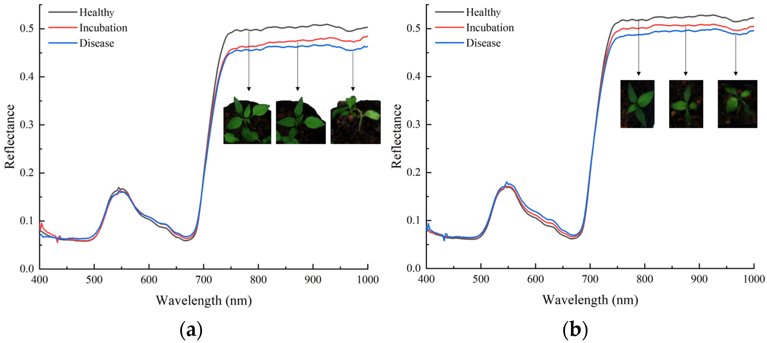
3.1. Analysis of Spectral Properties

Figure 2 displays the mean spectral standard deviation curve of chili pepper in the wavelength range of 400 to 1000 nm, together with its related leaf condition. The findings indicated minimal disparity in the spectral curve patterns between the two varieties of chili pepper samples. The dissimilarity primarily manifested within the wavelength intervals of 550–650 nm and 750–850 nm. The spectral information within the wavelength range of 550–650 nm is commonly employed to assess vegetation attributes, such as vegetative growth and health, and can be utilized to quantify chlorophyll concentration. As can be seen in Figure 2b, the spectral reflectance of the samples in the diseased period of Shanjiao No. 4 decreased more obviously, indicating that the samples in the diseased period were significantly different from other samples, and more chlorophyll may be lost under the stress of root rot. Figure 2a shows that the reflectance of Manshanhong leaf samples during the incubation period increased from low to high within the wavelength range of 750–850 nm. The spectral reflectance of the incubation period samples differed significantly from both the healthy period samples and the diseased period samples. This difference may be attributed to the high-water loss during the incubation period, which resulted in a large disparity between the healthy and incubation period leaves of this variety of chili peppers. The spectral reflectance of the leaf samples during the incubation period of Shanjiao No. 4 was rather mild. Compare Figure 2a,b, the spectral curves of these two pepper varieties have similar trends, and in order to increase the robustness of the model, the hyperspectral data of the two pepper varieties were blended to model. In this way, it can increase the portability of the early detection model of disease, so that the experimental results of this study can be applied to other chili pepper varieties.

3.2. Effective Wavelength Selection

SPA is used to select the most effective wavelengths from the full spectral data to reduce redundant variables. The number of effective wavelengths is set to range from 10 to 32. After repeated tests, when the number of variables is 13, the combination of effective wavelengths used has the smallest corrected RMSE (RMSE = 0.2797). The final selected effective wavelengths are 425, 433, 437, 453, 552, 639, 670, 680, 690, 715, 741, 819, and 909 nm, accounting for 5.08% of all bands.

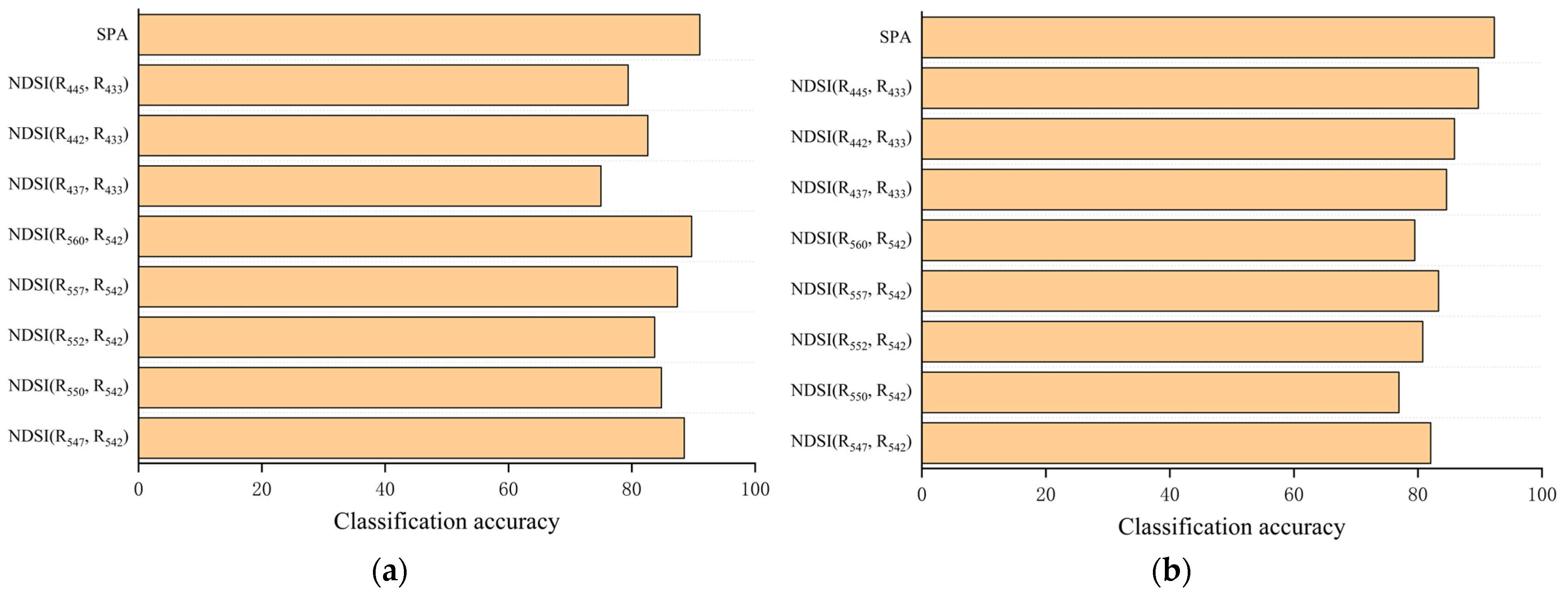
3.3. Correlation Analysis of Spectral Index

All chili pepper samples were classed by health, incubation, and diseased periods. The Pearson correlation coefficient was used to assess the NDSI values obtained from the reflectivity of chili pepper leaf samples at any two wavelengths ranging from 400 nm to 1000 nm. The correlation coefficient was plotted into a distribution matrix, as shown in Figure 3. The Pearson correlation coefficient is a method to measure the linear relationship between two continuous variables. Pearson correlation coefficient is widely used in data analysis and machine learning, such as feature selection, data preprocessing, and model evaluation. The value of the Pearson correlation coefficient ranges from −1 to 1. When the two variables are completely positively correlated, the value is 1; when the two variables are completely negatively correlated, the value is −1; when the two variables do not have any linear relationship, the value is 0.

The results are shown in Figure 3. The red area shows the highest positive correlation value and the blue area shows the highest negative correlation value. The spectral index constructed in the wavelength range of 560~610 nm and near showed a high correlation with root rot. The spectral index constructed in the wavelength range of 790~810 nm and near had a high correlation with root rot. The absolute value of the correlation coefficient in this region was significantly lower than that in the wavelength range of 560~610 nm, and the maximum value of the absolute value of the correlation coefficient was 0.725. The correlation between the spectral index constructed in other regions and root rot was generally low, and the range of correlation coefficient was 0 to 0.3. The results showed that the sensitive bands related to chili pepper root rot were mainly distributed in the bands of 560~610 nm and 560~610 nm.

Within the correlation coefficient distribution map, we identified eight spectral indices that displayed the greatest absolute association with chili pepper root rot leaves. We then determined the band combination of these spectral indices and recorded their respective correlation coefficients. The findings are displayed in

Table 1. Eight spectral indices with the highest absolute value of correlation coefficient with chili pepper root rot leaves.

Wavelength Combination	Spectral Index	Correlation Coefficient
R547, R542	NDSI (R547, R542)	0.911
R550, R542	NDSI (R550, R542)	0.887
R552, R542	NDSI (R552, R542)	0.894
R557, R542	NDSI (R557, R542)	0.898
R560, R542	NDSI (R560, R542)	0.909
R437, R433	NDSI (R437, R433)	0.896
R442, R433	NDSI (R442, R433)	0.883
R445, R433	NDSI (R445, R433)	0.887

.

3.4. Early Disease Detection Model

3.4.1. PLS-DA Model Based on Effective Wavelength

Due to the requirement of having more independent factors than dependent variables in PLS modeling, it is not feasible to utilize the PLS-DA model for testing the impact of spectral index. Therefore, only the SPA-PLS-DA model is constructed. When developing the SPA-PLS-DA model, the cross-validation technique is commonly employed to compute the root mean square error (RMSE) across several latent variables (LVs). The appropriate number of latent variables (LVs) for cross-validation was discovered by comparing the root mean square error (RMSE) values across different LVs. The model achieves optimality when there are exactly six potential variables, and the corresponding root mean square error (RMSE) is 0.291.

Figure 4a is the confusion matrix of the training results of the prediction set of the SPA-PLS-DA model of spectral data of 13 effective wavelengths established by 10-fold cross-validation. Among the 26 healthy period samples, 3 were misjudged as incubation period, with an accuracy rate of 88.5%. Among the 26 incubation period samples, 3 were misjudged as healthy periods, with an accuracy rate of 88.5%. One of the 26 diseased period samples was misjudged as the incubation period, with an accuracy rate of 96.2%. Overall, the TC of the prediction set was 91.1%. By analyzing the above data, it can be known that the healthy period leaves and the incubation period leaves are easily confused in the recognition, and the prediction results of the diseased period leaves are satisfactory.

3.4.2. LSSVM Model

In order to determine the optimal spectral index and assess the impact of effective wavelength modeling, the spectral reflectance data of chili pepper leaf samples at various infection stages were utilized. The values and effective wavelength variables of the top eight spectral indexes, which exhibited the strongest correlation, were calculated. Additionally, a discriminant analysis using the LSSVM model was conducted to establish a relationship between the disease stage of chili pepper leaves and the corresponding spectral indexes. The model parameters of LSSVM are set as type = classification problem. Linear kernel function = ‘lin_kernel’; kernel function parameter = 1; gaussian kernel function parameter = 1; polynomial kernel function parameter = 2; penalty factor = 1; lagrangian relaxation variable = 0.1; the results of the prediction set of the model are shown in Figure 5a.

As can be seen in Figure 5a, the classification accuracy of the prediction set of the NDSI (R₄₃₇, R₄₃₃)-LSSVM model is 75%, which is the lowest among the eight spectral index combinations. NDSI (R₅₆₀, R₅₄₂)-LSSVM model had the highest prediction accuracy with a TC of 89.1% for the prediction set. Therefore, the selected spectral index was proved to be suitable for the establishment of an early classification model of chili pepper root rot, which could identify whether chili pepper seedlings were diseased at the early stage of chili pepper seedling infection. Compared with the SPA-LSSVM model (TC = 91.03%), there is a certain gap. This is because the spectral index contains too few variables, so some important features are lost, so the modeling accuracy is lower than the effect of using characteristic wavelengths. Figure 4b shows the training results of the prediction set of the SPA-LSSVM model, which is the best result among the individual models modeled using the LSSVM model. Three of the 26 healthy period samples were misjudged as the incubation period, and four of the 26 incubation period samples were misjudged as the healthy period. Figure 4c shows the training results of the prediction set of NDSI (R₅₆₀, R₅₄₂)-LSSVM, which has the highest accuracy among the LSVM models modeled based on spectral indices. Among the 26 healthy period samples, 3 were misjudged as the incubation period, with an accuracy rate of 88.5%. Among the 26 incubation period samples, 2 were misjudged as healthy period and 2 were misjudged as diseased period, with an accuracy rate of 84.6%. One of the 26 diseased period samples was misjudged as an incubation period, with an accuracy rate of 96.2%. Overall, the TC of the prediction set is 89.7%. It is worth mentioning that in the LSSVM model based on the spectral index, the misjudgment of the disease period is mostly the red chili pepper variety. In this interval, the difference between the diseased period samples of the fourth chili pepper and other samples is greater, so it is easier to distinguish, which can also prove that the difference in the spectrum can be used to classify. The NDSI (R₅₆₀, R₅₄₂)-LSSVM model has similar classification accuracy with the SPA-LSSVM model, and at the same time reduces the parameters required for modeling. Only two wavelengths of spectral reflectance data are used, which is more conducive to the application of spectral technology-based detectors at the moment when spectrometers and narrow-band filters are expensive.

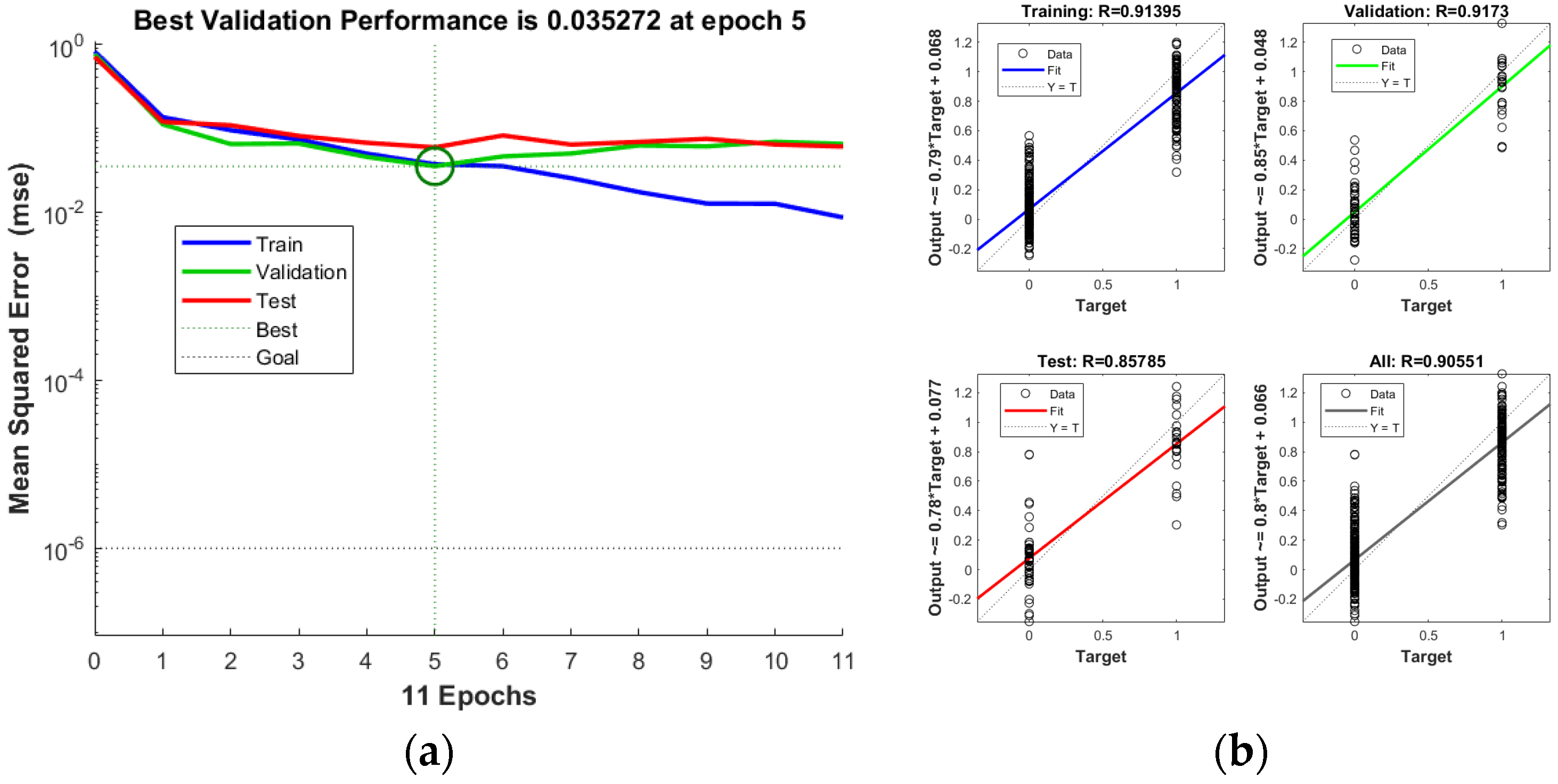
3.4.3. BP Neural Network

To further verify the advantages and disadvantages of spectral index and modeling based on the effective wavelength method, this paper designs a BP neural network model. The whole BP neural network model is composed of an input, hidden layer, output layer, and output. The activation function of the hidden layer is set to tansig, and the activation function of the output layer is set to purelin. The maximum number of iterations in the training parameters is set to 10,000, the target training error is set to 10⁻⁶, and the learning rate is set to 0.01. The entire BP network uses the Levenberg–Marquardt training algorithm, the validation checks are set to 6, and the data classification method is set to random. Finally, after several debugging, the training results of the prediction set of the model are shown in Figure 5b. The effect of the SPA-BP model is slightly better than the BP model that based on spectral index modeling. The TC of the SPA-BP model is 92.3%. The best combination of spectral index is NDSI (R₄₄₅, R₄₃₃), and the TC of NDSI (R₄₄₅, R₄₃₃)-BP model is 89.7%. It can be seen from Figure 6a,b that the SPA-BP model has a total of 11 iterations, and the best verification performance is achieved when the epoch is 5, and the mean square error is 0.0353. The mean square error represents the expected value of the difference between the predicted output and the target output, and the closer it is to 0, the better. The regression value R represents the correlation between the predicted output and the target output. The closer R is to 1, the closer the relationship between the predicted value and the actual value is. The closer R is to 0, the greater the randomness of the relationship between the predicted and output data is. The R of the training set, validation set, and test set of the SPA-BP model after training are 0.914, 0.917, and 0.858, respectively, indicating that there is a strong positive correlation between the predicted classification and the actual classification. It can be seen from Figure 6c,d that the NDSI (R₄₄₅, R₄₃₃)-BP model performed a total of 10 iterations, and achieved the best verification performance at epoch 4, with a mean square error of 0.0599. The R of the training set, validation set, and test set of the SPA-BP model after training is 0.9,0.855, and 0.832, respectively, and the model performance is excellent. The specific training results are shown in Figure 4d,e of the confusion matrix. Figure 4d is the classification result of the SPA-BP model. Among them, 3 of 29 healthy period samples were misjudged as incubation period samples, 2 of 28 incubation period samples were misjudged as healthy period samples, and 21 diseased period samples were misjudged as incubation period samples. Figure 4e is the classification result of the NDSI (R₄₄₅, R₄₃₃)-BP model. Two of the 27 healthy period samples were misjudged as incubation period samples, five of the 29 incubation period samples were misjudged as healthy period samples, and one was misjudged as diseased period samples. Most of the misjudgments between the incubation period and the healthy period of the leaves are the chili peppers of the Shanjiao No. 4 variety of chili pepper, and the number of misjudgments is 5 (a total of 7). Only two are the chili peppers of the Manshanhong variety. The disparity in the duration of the incubation phase and the healthy period of the Manshanhong chili pepper appears to be more significant compared with the Shanjiao No. 4 variety of chili pepper, thus aligning with the hypothesis stated in Section 3.1. Furthermore, akin to the LSSVM algorithm, the primary misjudgment in the samples predominantly occurs between the healthy period sample and the incubation period sample. There is no discernible distinction between samples taken during a healthy time and ones taken during the incubation phase, and the variations between them are extremely minimal. Nevertheless, hyperspectral imaging technology has the capability to catch the internal variations inside the leaves of chili pepper plants. The results demonstrate that the classification model utilizing hyperspectral imaging exhibits superior capability in early diagnosis of chili pepper root rot.

4. Discussion

Overall, this study achieved the expected results. The results of the study were able to demonstrate the potential of hyperspectral imaging in detecting chili root rot. Starting from the laboratory inoculation of chill root rot pathogens, it could be noticed that chili seedlings that were deliberately inflicted with the pathogen were diseased. No symptoms were visible to the unaided eye on the initial day of injection. On the second day following inoculation, both varieties of chili pepper seedlings exhibited characteristic indications of root rot, including leaf wilting, shrinkage of the stem base, and minor stem lodging. By the third day after inoculation, the chili pepper seedlings exhibited severe leaf shrinkage and a dark brown coloration at the stem base, resulting in the collapse and death of the seedlings. The incidence mirrored the findings of Tada Terufumi, who observed a mortality rate above 82% in seedlings three days after being inoculated with root rot [39]. Therefore, according to the period of onset of chili, it is divided into three phases: healthy, incubation and diseased.

Hyperspectral imaging is able to capture differences in the reflectance of chili peppers at different times, differences that are difficult to detect by the human eye. These differences between spectral reflectance are the basis on which classification models can be created. Observing Figure 2, it is not difficult to find a clear difference in the spectral reflectance of healthy and diseased chili pepper leaves in the wavelength ranges of 550 nm, 580 to 680 nm, and 760 to 1000 nm. This significant difference confirms the effectiveness of hyperspectral imaging in identifying leaf lesions [40]. Further analysis showed that chili pepper leaf reflectance was highest in the healthy phase and much lower in the diseased period than in the incubation period. In the range of 580~680 nm, the reflectivity of leaves in the healthy period was low, and the reflectivity in this range gradually decreased with the aggravation of the disease. The near-infrared band spectral reflectance of infected leaves (including the incubation period and the diseased period) was significantly lower than that of healthy leaves.

Hyperspectral cameras capture hundreds of wavelengths, but some wavelengths reflect very little information about the disease, and modelling using all of them would make the model too large. In general, dimensionality reduction of spectral data is necessary. Selecting effective wavelengths and spectral indices are common methods for dimensionality reduction, and strictly speaking, spectral indices are also a form of selecting effective wavelengths. Unlike the direct selection of effective wavelengths, spectral indices construct mathematical equations by combining between different wavelengths. The advantage of using effective wavelength downscaling is that it covers more complete spectral data and the identification accuracy after modelling is generally slightly higher, and the advantage of using spectral index modelling is that fewer wavelength bands are required. It can be seen from this study that the results of modelling using the SPA method are all superior to those modelled using NDSI. But whichever way the modelling is done, the modelling accuracy can be in line with the desired goal.

This study explored the potential application of hyperspectral imaging for chili root rot detection and provided a theoretical basis for the development of a portable chili root rot detector. Future research needs to be carried out in the following areas: comparing the newly created spectral index with the traditional vegetation index is used to validate the excellence of the spectral index created in this study; the reflectance of chili root rot varies between different varieties of chili, and more varieties of chili will be covered in future studies to improve the robustness of the model; and the use of hyperspectral imaging to explore the pathogenesis of chili root rot from a microscopic point of view The study will be carried out in the following years.

5. Conclusions

This work employed hyperspectral imaging to identify chili root rot, demonstrating its significant potential for non-destructive and expedient detection of this disease. The dimensionality of hyperspectral information was reduced using the SPA algorithm and spectral index method, and the reduced spectral and disease information were input into the classification algorithm to obtain the best classification model. The R of the trained SPA-BP model for the training, validation and test sets are 0.91395, 0.9173, and 0.85785, respectively, and the classification accuracy for the prediction set can be up to 92.3%, which is the best result among all classification models. However, from a practical application point of view, the SPA method requires too many bands and is not conducive to the design of low-cost field chili root rot detection instruments. It is worth mentioning that the R of the trained NDSI (R₄₄₅, R₄₃₃)-BP model for the training, validation, and test sets were 0.89591, 0.85459, and 0.83176, respectively. the classification accuracy of the prediction set was 89.7426%, which also achieves a better prediction accuracy and the spectral index method requires only two bands to detect the root rot disease, which It can improve the efficiency of real-time instrumental detection. This study can provide a theoretical basis and technical support for the early detection of chili pepper root rot by hyperspectral imaging technology.

References

1. Rong, H.; Guo, D.; Yang, W.; Dai, W.; Yang, J.; Liou, X. Isolation and identification of the pathogen of capsicum root rot in Tibet. Acta Agric. Boreali Occi Dent. Sin. 2015, 24, 139–143. [Google Scholar]
2. Gustafson, L.L.; Arzul, I.; Burge, C.A.; Carnegie, R.B.; Caceres-Martinez, J.; Creekmore, L.; Dewey, W.; Elston, R.; Friedman, C.S.; Hick, P.; et al. Optimizing surveillance for early disease detection: Expert guidance for Ostreid herpesvirus surveillance design and system sensitivity calculation. Prev. Vet. Med. 2021, 194, 105419. [Google Scholar] [CrossRef]
3. Debnath, O.; Saha, H.N. An IoT-based intelligent farming using CNN for early disease detection in rice paddy. Microprocess. Microsyst. 2022, 94, 104631. [Google Scholar] [CrossRef]
4. Gao, Z.; Khot, L.R.; Naidu, R.A.; Zhang, Q. Early detection of grapevine leafroll disease in a red-berried wine grape cultivar using hyperspectral imaging. Comput. Electron. Agric. 2020, 179, 105807. [Google Scholar] [CrossRef]
5. Shao, Y.; Liu, Y.; Xuan, G.; Shi, Y.; Li, Q.; Hu, Z. Detection and analysis of sweet potato defects based on hyperspectral imaging technology. Infrared Phys. Technol. 2022, 127, 104403. [Google Scholar] [CrossRef]
6. Sharma, M.; Jindal, V. Approximation techniques for apple disease detection and prediction using computer enabled technologies: A review. Remote Sens. Appl. Soc. Environ. 2023, 32, 101038. [Google Scholar] [CrossRef]
7. Daniya, T.; Vigneshwari, S. Rider Water Wave-enabled deep learning for disease detection in rice plant. Adv. Eng. Softw. 2023, 182, 103472. [Google Scholar] [CrossRef]
8. Khan, A.I.; Quadri, S.M.K.; Banday, S.; Latief Shah, J. Deep diagnosis: A real-time apple leaf disease detection system based on deep learning. Comput. Electron. Agric. 2022, 198, 107093. [Google Scholar] [CrossRef]
9. Allen, B.; Dalponte, M.; Ørka, H.O.; Næsset, E.; Puliti, S.; Astrup, R.; Gobakken, T. UAV-Based Hyperspectral Imagery for Detection of Root, Butt, and Stem Rot in Norway Spruce. Remote Sens. 2022, 14, 3830. [Google Scholar] [CrossRef]
10. Adam, E.; Deng, H.; Odindi, J.; Abdel-Rahman, E.M.; Mutanga, O. Detecting the Early Stage of Phaeosphaeria Leaf Spot Infestations in Maize Crop Using In Situ Hyperspectral Data and Guided Regularized Random Forest Algorithm. J. Spectrosc. 2017, 2017, 6961387. [Google Scholar] [CrossRef]
11. Ba, W.; Jin, X.; Lu, J.; Rao, Y.; Zhang, T.; Zhang, X.; Zhou, J.; Li, S. Research on predicting early Fusarium head blight with asymptomatic wheat grains by micro-near infrared spectrometer. Spectrochim. Acta Part A: Mol. Biomol. Spectrosc. 2023, 287, 122047. [Google Scholar] [CrossRef]
12. Chen, B.; Li, S.-K.; Wang, K.-R.; Wang, J.; Wang, F.-Y.; Xiao, C.-H.; Lai, J.-C.; Wang, N. Spectrum Characteristics of Cotton Canopy Infected with Verticillium Wilt and Applications. Agric. Sci. China 2008, 7, 561–569. [Google Scholar] [CrossRef]
13. Abdulridha, J.; Ampatzidis, Y.; Qureshi, J.; Roberts, P. Laboratory and UAV-Based Identification and Classification of Tomato Yellow Leaf Curl, Bacterial Spot, and Target Spot Diseases in Tomato Utilizing Hyperspectral Imaging and Machine Learning. Remote Sens. 2020, 12, 2732. [Google Scholar] [CrossRef]
14. Calamita, F.; Imran, H.A.; Vescovo, L.; Mekhalfi, M.L.; La Porta, N. Early Identification of Root Rot Disease by Using Hyperspectral Reflectance: The Case of Pathosystem Grapevine/Armillaria. Remote Sens. 2021, 13, 2537. [Google Scholar] [CrossRef]
15. Wei, X.; He, J.; Zheng, S.; Ye, D. Modeling for SSC and firmness detection of persimmon based on NIR hyperspectral imaging by sample partitioning and variables selection. Infrared Phys. Technol. 2020, 105, 103099. [Google Scholar] [CrossRef]
16. Galvão, R.K.H.; Araujo, M.C.U.; José, G.E.; Pontes, M.J.C.; Silva, E.C.; Saldanha, T.C.B. A method for calibration and validation subset partitioning. Talanta 2005, 67, 736–740. [Google Scholar] [CrossRef]
17. Li, Y.; Fang, T.; Zhu, S.; Huang, F.; Chen, Z.; Wang, Y. Detection of olive oil adulteration with waste cooking oil via Raman spectroscopy combined with iPLS and SiPLS. Spectrochim. Acta Part A Mol. Biomol. Spectrosc. 2018, 189, 37–43. [Google Scholar] [CrossRef]
18. Tian, H.; Zhang, L.; Li, M.; Wang, Y.; Sheng, D.; Liu, J.; Wang, C. Weighted SPXY method for calibration set selection for composition analysis based on near-infrared spectroscopy. Infrared Phys. Technol. 2018, 95, 88–92. [Google Scholar] [CrossRef]
19. Sun, J.; Zhou, X.; Hu, Y.; Wu, X.; Zhang, X.; Wang, P. Visualizing distribution of moisture content in tea leaves using optimization algorithms and NIR hyperspectral imaging. Comput. Electron. Agric. 2019, 160, 153–159. [Google Scholar] [CrossRef]
20. Song, Y.; Cao, S.; Chu, X.; Zhou, Y.; Xu, Y.; Sun, T.; Zhou, G.; Liu, X. Non-destructive detection of moisture and fatty acid content in rice using hyperspectral imaging and chemometrics. J. Food Compos. Anal. 2023, 121, 105397. [Google Scholar] [CrossRef]
21. Datt, B. A New Reflectance Index for Remote Sensing of Chlorophyll Content in Higher Plants: Tests using Eucalyptus Leaves. J. Plant Physiol. 1999, 154, 30–36. [Google Scholar] [CrossRef]
22. Daughtry, C.S.T.; Hunt, E.R.; McMurtrey, J.E. Assessing crop residue cover using shortwave infrared reflectance. Remote Sens. Environ. 2004, 90, 126–134. [Google Scholar] [CrossRef]
23. Chen, T.; Zhang, J.; Chen, Y.; Wan, S.; Zhang, L. Detection of peanut leaf spots disease using canopy hyperspectral reflectance. Comput. Electron. Agric. 2019, 156, 677–683. [Google Scholar] [CrossRef]
24. Zhang, Y.; Wu, J.; Wang, A. Comparison of various approaches for estimating leaf water content and stomatal conductance in different plant species using hyperspectral data. Ecol. Indic. 2022, 142, 109278. [Google Scholar] [CrossRef]
25. Yao, X.; Zhu, Y.; Tian, Y.; Feng, W.; Cao, W. Exploring hyperspectral bands and estimation indices for leaf nitrogen accumulation in wheat. Int. J. Appl. Earth Obs. Geoinf. 2010, 12, 89–100. [Google Scholar] [CrossRef]
26. Zhao, M.; Cang, H.; Chen, H.; Zhang, C.; Yan, T.; Zhang, Y.; Gao, P.; Xu, W. Determination of quality and maturity of processing tomatoes using near-infrared hyperspectral imaging with interpretable machine learning methods. LWT 2023, 183, 114861. [Google Scholar] [CrossRef]
27. Peerbhay, K.Y.; Mutanga, O.; Ismail, R. Commercial tree species discrimination using airborne AISA Eagle hyperspectral imagery and partial least squares discriminant analysis (PLS-DA) in KwaZulu–Natal, South Africa. ISPRS J. Photogramm. Remote Sens. 2013, 79, 19–28. [Google Scholar] [CrossRef]
28. Cucuzza, P.; Serranti, S.; Capobianco, G.; Bonifazi, G. Multi-level color classification of post-consumer plastic packaging flakes by hyperspectral imaging for optimizing the recycling process. Spectrochim. Acta Part A Mol. Biomol. Spectrosc. 2023, 302, 123157. [Google Scholar] [CrossRef]
29. Cruz-Tirado, J.P.; Lima Brasil, Y.; Freitas Lima, A.; Alva Pretel, H.; Teixeira Godoy, H.; Barbin, D.; Siche, R. Rapid and non-destructive cinnamon authentication by NIR-hyperspectral imaging and classification chemometrics tools. Spectrochim. Acta Part A Mol. Biomol. Spectrosc. 2023, 289, 122226. [Google Scholar] [CrossRef]
30. Zhang, W.; Pan, L.; Lu, L. Prediction of TVB-N content in beef with packaging films using visible-near infrared hyperspectral imaging. Food Control 2023, 147, 109562. [Google Scholar] [CrossRef]
31. Xu, M.; Sun, J.; Yao, K.; Cai, Q.; Shen, J.; Tian, Y.; Zhou, X. Developing deep learning based regression approaches for prediction of firmness and pH in Kyoho grape using Vis/NIR hyperspectral imaging. Infrared Phys. Technol. 2022, 120, 104003. [Google Scholar] [CrossRef]
32. Cheng, L.; Liu, G.; He, J.; Wan, G.; Ma, C.; Ban, J.; Ma, L. Non-destructive assessment of the myoglobin content of Tan sheep using hyperspectral imaging. Meat Sci. 2020, 167, 107988. [Google Scholar] [CrossRef]
33. Wang, Y.; Song, S. Variety identification of sweet maize seeds based on hyperspectral imaging combined with deep learning. Infrared Phys. Technol. 2023, 130, 104611. [Google Scholar] [CrossRef]
34. Wang, T.; Gao, M.; Cao, C.; You, J.; Zhang, X.; Shen, L. Winter wheat chlorophyll content retrieval based on machine learning using in situ hyperspectral data. Comput. Electron. Agric. 2022, 193, 106728. [Google Scholar] [CrossRef]
35. Ma, J.; Cheng, J.; Wang, J.; Pan, R.; He, F.; Yan, L.; Xiao, J. Rapid detection of total nitrogen content in soil based on hyperspectral technology. Inf. Process. Agric. 2022, 9, 566–574. [Google Scholar] [CrossRef]
36. Zhao, J.; Yan, H.; Huang, L. A joint method of spatial–spectral features and BP neural network for hyperspectral image classification. Egypt. J. Remote Sens. Space Sci. 2023, 26, 107–115. [Google Scholar] [CrossRef]
37. Li, Z.; Ni, C.; Wu, R.; Zhu, T.; Cheng, L.; Yuan, Y.; Zhou, C. Online small-object anti-fringe sorting of tobacco stem impurities based on hyperspectral superpixels. Spectrochim. Acta Part A Mol. Biomol. Spectrosc. 2023, 302, 123084. [Google Scholar] [CrossRef]
38. An, J.; Zhang, C.; Zhou, L.; Jin, S.; Zhang, Z.; Zhao, W.; Pan, X.; Zhang, W. Tensor based low rank representation of hyperspectral images for wheat seeds varieties identification. Comput. Electr. Eng. 2023, 110, 108890. [Google Scholar] [CrossRef]
39. Tada, T.; Tanaka, C.; Katsube-Tanaka, T.; Shiraiwa, T. Effects of wounding and relative humidity on the incidence of Phytophthora root and stem rot in soybean seedlings. Physiol. Mol. Plant Pathol. 2021, 116, 101737. [Google Scholar] [CrossRef]
40. Zhang, J.; Tian, Y.; Yan, L.; Wang, B.; Wang, L.; Xu, J.; Wu, K. Diagnosing the symptoms of sheath blight disease on rice stalk with an in-situ hyperspectral imaging technique. Biosyst. Eng. 2021, 209, 94–105. [Google Scholar] [CrossRef]
Figure 1. The processing flow chart of using mask to extract the region of interest.
Agronomy 14 00226 g001
Figure 2. The average spectral curve and leaf status of different varieties of chili pepper leaves at different infection stages: (a) Manshanhong; (b) Shanjiao No. 4.
Agronomy 14 00226 g002
Figure 3. The correlation coefficient distribution of NDSI values was calculated by any two wavelengths at different infection stages of chili pepper leaves.
Agronomy 14 00226 g003
Figure 4. The confusion matrix of the training results of the prediction set of each model (a): SPA-PLS-DA model; (b): SPA-LSSVM model; (c): NDSI (R560, R542)-LSSVM model; (d): SPA-BP model; (e): NDSI (R445, R433)-BP model.
Agronomy 14 00226 g004
Figure 5. Model classification accuracy based on SPA effective wavelength and eight spectral indices (a): LSSVM model; (b): BP neural network.
Agronomy 14 00226 g005
Figure 6. (a) (SPA-BP model), (c) (NDSI (R445, R433)-BP model) are images of the mean square error versus the number of training times, and (b) (SPA-BP model), (d) (NDSI (R445, R433)-BP model) are the gradient plots of the correlation between the predicted values and the actual values, respectively. The “output ~= Numbers*Target + Numbers” in Figures (b,d) characterize the regression line equations, with “ * ” denoting multiplication.
Agronomy 14 00226 g006aAgronomy 14 00226 g006b