Article

Estimation of Spring Maize Planting Dates in China Using the Environmental Similarity Method

1
Institute of Digital Agriculture, Zhejiang Academy of Agricultural Sciences, Hangzhou 310021, China
2
Key Laboratory of Information Traceability for Agricultural Products, Ministry of Agriculture and Rural Affairs of China, Hangzhou 310021, China
3
Key Laboratory of Virtual Geographic Environment, Nanjing Normal University, Ministry of Education, Nanjing 210023, China
4
State Key Laboratory Cultivation Base of Geographical Environment Evolution, Nanjing 210023, China
5
Department of Geography, University of Wisconsin-Madison, Madison, WI 53706, USA
*
Author to whom correspondence should be addressed.
Agronomy 2024, 14(1), 97; https://doi.org/10.3390/agronomy14010097
Submission received: 4 December 2023 / Revised: 25 December 2023 / Accepted: 27 December 2023 / Published: 30 December 2023
(This article belongs to the Topic Advances in Crop Simulation Modelling)

Abstract

:
Global climate change is a serious threat to food and energy security. Crop growth modelling is an important tool for simulating crop food production and assisting in decision making. Planting date is one of the important model parameters. Larger-scale spatial distribution with high accuracy for planting dates is essential for the widespread application of crop growth models. In this study, a planting date prediction method based on environmental similarity was developed in accordance with the third law of geography. Spring maize planting date observations from 124 agricultural meteorological experiment stations in China over the years 1992–2010 were used as the data source. Samples spanning from 1992 to 2009 were allocated as training data, while samples from 2010 constituted the independent validation set. The results indicated that the root mean square error (RMSE) for spring maize planting date based on environmental similarity was 10 days, which is better than that of multiple regression analysis (RMSE = 13 days) in 2010. Additionally, when applied at varying scales, the accuracy of national-scale prediction was better than that of regional-scale prediction in areas with large differences in planting dates. Consequently, the method based on environmental similarity can effectively and accurately estimate planting date parameters at multiple scales and provide reasonable parameter support for large-scale crop growth modelling.

1. Introduction

The increasing global population and the impact of climate change have made food security a pressing global challenge [1,2,3]. Maize (Zea mays L.) is a primary global crop, serving not only as a staple food but also utilized for corn ethanol, animal feed, and various other purposes [4]. China’s maize production constitutes 25.52% of the world’s total output, reaching approximately 277.20 million tons in 2022 from a sowing area of 43.07 million hectares [5,6]. Accurately estimating China’s maize yield is therefore crucial for ensuring global food security.
Process-based crop models serve as primary scientific tools for estimating crop yield, assessing the impact of environmental changes, and guiding adaptive measures under climate change [4,7,8]. Crop productivity is intricately linked to crop phenology [9,10], which is significantly influenced by climate, including changes due to warming trends [11,12,13,14,15]. In the phenological stages of crops, the timing of planting significantly impacts crop productivity [16,17,18]. To adapt to climate change and enhance productivity, farmers must employ various strategies, such as altering planting schedules [19,20,21,22]. Consequently, for most process-based crop models, the planting date (PD) stands as a key input for management decisions [22,23,24]. This aspect has been identified as a primary source of uncertainty in model outcomes [25,26].
There are many methods for estimating planting dates. The first relies on spatial autocorrelation, employing various interpolation techniques like inverse distance weighting (IDW) [27,28], radial basis functions (RBF) [29], and Kriging [30]. However, these methods assume stationary spatial autocorrelation, which might not be fully applicable in cases involving complex geographic processes. For instance, Gerstmann et al. [30] highlighted considerable uncertainty in predictions within mountainous regions. This is because planting dates are influenced by numerous environmental factors such as temperature, precipitation, soil moisture, and labor availability. Therefore, estimating planting dates can rely on these environmental variables. Statistical methods for predicting planting dates include rule-based approaches [19,24,31,32], regression analysis [23,33,34], and machine learning techniques [35]. Typically, these methods involve applying fixed rules, thresholds, or functions across the entire study area. However, the relationships between planting dates and environmental factors vary across locations and over time within different regions [36].
These methods are limited by their reliance on fixed spatial autocorrelation relationships, functions, or rules to model planting date variations. There is a clear need for new techniques in spatially predicting planting dates that do not require the extracted relationships to adhere to stationary conditions. To address these limitations, this paper introduces a method based on geographic environment similarity (the third law of geography) [37] for spatially predicting maize planting dates. The theoretical framework based on geographic environmental similarity is articulated in the third law of geography [37]. It can be summarized simply as: the more alike the geographic environment between two locations, the more similar their geographic features. This principle has found application in various research domains, including soil type mapping [38], assessment of soil organic matter [39], and so on. Therefore, considering the correlation between planting dates and environmental factors, locations sharing similar environmental conditions are likely to have similar planting date values.
In this study, the environmental similarity method was applied to predict spring maize planting date and compared with the multiple linear regression method. Our aim is to find a highly accurate method for predicting planting dates on a large scale and to validate and discuss this method. Section 2 presents the materials and the environmental similarity method of this study. It mainly describes the method setup, evaluation, and validation. The results and discussion are presented in Section 3. The conclusions are presented in Section 4.

2. Materials and Methods

2.1. Study Area and Datasets

The study areas include five primary spring maize cultivation zones in China, delineated based on soil and climate characteristics. These zones consist of northeast China (NE), Inner Mongolia Autonomous Region north of the Great Wall (IMA), northwest China (NW), Loess Plateau China (LP), and southwest China (SW). Planting dates were obtained from observed records at 124 agricultural meteorological experiment stations under the Chinese Meteorological Administration (CMA), spanning the period from 1992 to 2010, resulting in a total of 1520 observation samples (Figure 1). These samples of planting dates have standardized observation guidelines [25]. Therefore, it can be assumed that the planting date is an optimal date in these experiment stations [12,34].
Climate data, including daily mean temperatures, minimum temperatures, and precipitation from 1992 to 2010 across 124 stations, were gathered from the CMA. Missing data at some stations were supplemented using a gridded climate product [40]. Daily climate data were aggregated on a monthly basis (February to June), comprising mean temperature and total monthly precipitation. A 1 km resolution digital elevation model (DEM) facilitated the computation of the slope gradient and relief amplitude using 5 × 5 neighborhood windows. For spatial prediction, climate and topographic factors were resampled to a spatial resolution of 0.25° × 0.25°.

2.2. Method

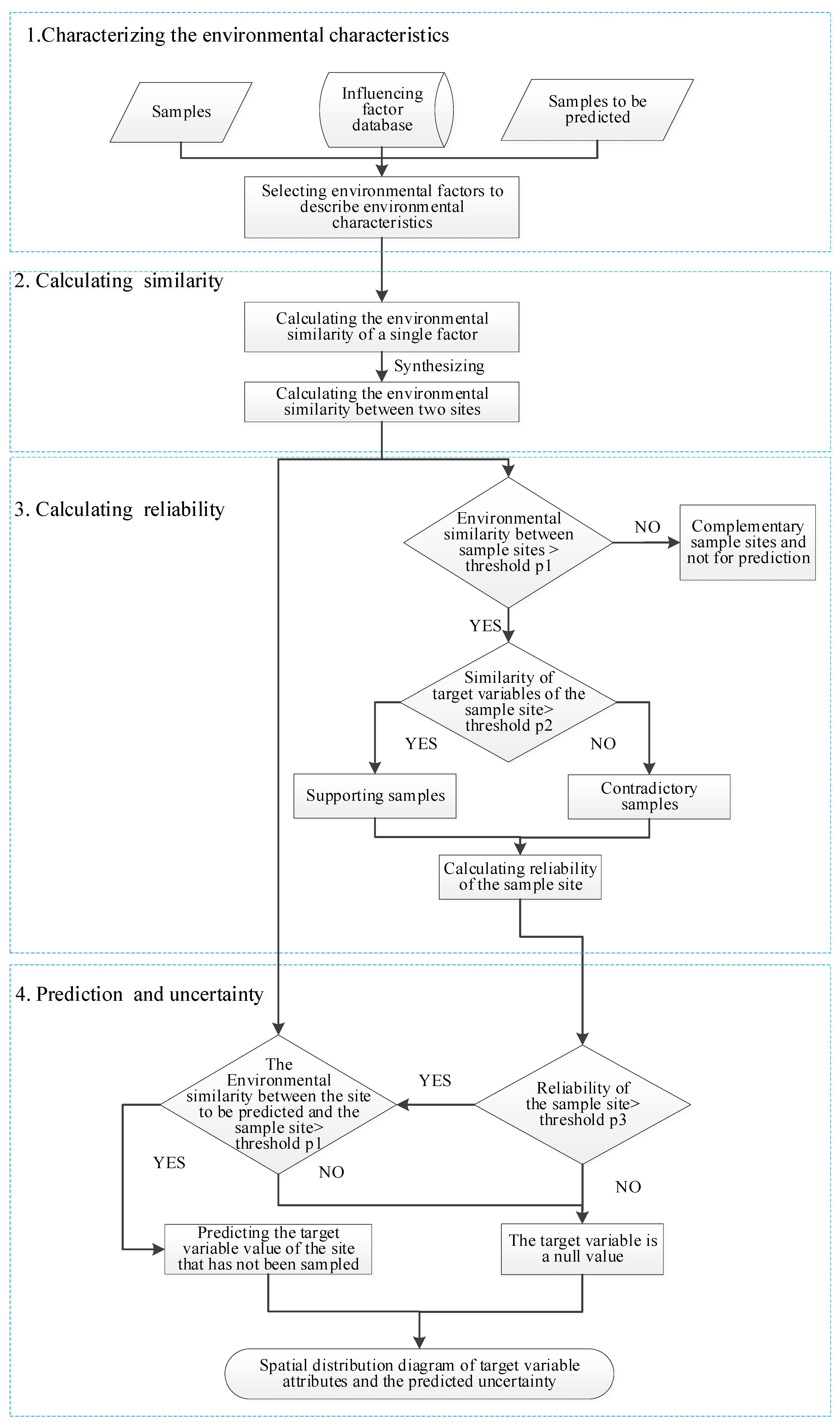
Four sequential steps are involved in spatially predicting PD based on environmental similarity (Figure 2). The initial step involves selecting environmental factors to depict the environmental characteristics related to the target variable (PD). Subsequently, the second step computes the environmental similarity between samples or between a sample and the prediction point. The third step entails assessing the credibility of each sample based on environmental similarity, selecting highly reliable samples for prediction. Finally, the fourth step involves predicting the target variable value and determining uncertainty values for the prediction points based on sample environmental similarity.
(1)
Characterizing the geographic environment associated with spring maize planting dates
Quantifying environmental conditions using planting dates at specific locations is crucial and imperative. Existing studies have primarily focused on establishing the correlation between planting dates and environmental factors in agricultural contexts. To capture the relationship between PD and environmental factors, climate covariates (including monthly mean temperature (T), monthly minimum temperature (Tmin), monthly precipitation (P), growing degree days above 8 °C (GDD8), and growing degree days above 10 °C (GDD10)) from February to June, along with topographic covariates (elevation, slope gradient, relief amplitude (RA)), were employed to characterize the environmental conditions.
(2)
Calculating environmental similarities
Environmental similarities are determined in two steps. Firstly, similarity values are calculated based on individual environmental covariates. In this study, we employed the Gower similarity coefficient [41] (Equation (1)).
E ( e v i , e v j ) = 1 e v i e v j R a n g e v
where E() represents the function evaluating the similarity of the individual environmental variable level; evi and evj are the values of the v-th environmental variable at location i and location j; and R a n g e v represents the value range of the v-th environmental variable.
Secondly, these similarities across all environmental variables are amalgamated into a single variable representing the overall similarity at a specific sample location. For this research, a minimum operator was utilized.
(3)
Calculating the reliability of each sample
The relationship between samples can be categorized into three types: supporting, contradictory, and supplementary samples, based on the similarity in environmental conditions and the target variable (planting dates). When samples share similar environmental conditions and exhibit similar target variable values, they are considered supportive. Higher support from multiple samples enhances the reliability of each individual sample.
The calculation of environmental and target variable similarity between samples constitutes the second step. The environmental similarity threshold (p1) and the target variable similarity threshold (p2) govern the relationships among sample points. A sample with solely contradictory points and lacking supportive ones is assigned a reliability of 0. If neither supportive nor contradictory points exist for a sample, its reliability is considered unknown and set as a value of “NA” (Equation (2)).
r i = k = 1 n s T S i , k n s × n s n s + n c   ,   n s + n c > 0   and   n s 0   0 ,   n c > 0   and   n s = 0   N A ,   n s + n c = 0
where r i represents the reliability of sample i; n s   and   n c represent the number of support samples and the number of contradictory samples for sample i, respectively; and T S i , k is the similarity of target variable between samples I and k.
(4)
Predicting planting date values and determining uncertainty
To establish the reliability threshold (p3) for samples, only those with high reliability are chosen for prediction. The planting date value at unsampled locations is forecasted using Equation (3).
V j = i = 1 n S j i × V i i = 1 n S j i
where n ' is the number of samples that met the prediction conditions; S j i is the environmental similarity between the unvisited location point j and the sample i; and V i is the target variable value (planting date) of the sample i.
The prediction uncertainty at each location correlates inversely with its environmental similarities and reliability with regard to existing samples. It is represented by the following equation:
U j = 1 m a x ( S j 1   ×   r 1 , S j 2   ×   r 2 ,   ,   S j n   ×   r n )
Equation (4) indicates that the prediction uncertainty at unvisited location j is affected by the environmental similarity (Sjn′) and reliability (rn′) at the sample points used in the prediction. Uncertainty is a measure of the degree of reliability in the environmental similarity model’s prediction results. The lower the uncertainty, the more credible the planting dates simulated by the model. The uncertainty value has no unit and is between 0 and 1. Uncertainty values closer to 1 mean that the model simulation results are less reliable, and values closer to 0 mean that the simulation results are reliable.

2.3. Evaluation and Validation

An independent validation sample set was utilized to assess prediction accuracy. In order to be consistent with the spatial prediction of the planting date of one year, samples spanning from 1992 to 2009 were allocated as training data, while samples from 2010 constituted the independent validation set. Table 1 presents the statistical values depicting the planting dates (day of the year) of spring maize in China for both the training and validation samples.
Four indices were used to evaluate prediction accuracy, including root mean square error (RMSE), mean absolute error (MAE), coefficient of determination ( R 2 ), and L5. The RMSE, MAE, and R 2 were defined as follows:
R M S E = i = 1 n y i ^ y i 2 n
M A E = 1 n i = 1 n y i ^ y i
R 2 = 1 i = 1 n y i y i ^ 2 i = 1 n ( y i y ¯ ) 2
where n represents validation points numbers, y i represents the PD value at location i, y i ^ represents the predicted value at location i, and y i ¯ and y i ^ ¯ are the means of y i and y i ^ , respectively. If the RMSE and MAE are close to 0 or R 2 is close to 1, then the model performs well.
Considering the planting date’s uniformity within farmers’ sowing periods and the vast crop area, slight variations occur in planting dates, especially under decentralized management practices in China. To better gauge predictive accuracy, this paper introduces a new metric named L5. L5 represents the percentage of sample points where the disparity between the predicted and actual planting dates is within 5 days. The calculation formula is as follows:
L5 = N5/N × 100
where N5 represents the number of sample points with an absolute value of less than 5 days between the predicted and the actual value. N represents the total number of sample points. If L5 is close to 100%, then the model performs well.
To compare the outcomes of environmental similarity prediction, same variables were used to predict planting dates using a multiple linear regression model [34]. To mitigate multicollinearity effects among the covariates, a principal component analysis (PCA) [42,43] was executed on the standardized environmental covariate values before constructing the multiple linear regression model (Table 2).
The regression process involved fitting the model using sequential principal components. The initial five principal components (PC1, PC2, PC3, PC4, and PC5) captured 86% of the variance in environmental covariates and were consequently chosen for constructing the multiple linear regression model (Equation (8)):
PD = 114.91 − 11.45 PC1 + 0.94 PC2 − 0.01 PC3 + 1.72 PC4 + 0.44 PC5 (R2 = 0.57)

3. Results and Discussion

3.1. Independent Validation Results

Table 3 shows the independent sample validation accuracies for both methods. Overall, the environmental similarity method exhibited lower RMSE (10 days) and MAE (8 days) values compared to the multiple regression method (RMSE = 13 days, MAE = 9 days). The L5 metric in the independent validation for the environmental similarity method stood at 37.5%, surpassing the multiple regression results (L5 = 31.9%). These findings suggest that the environmental similarity method outperformed the multiple regression method in accuracy.
Figure 3 shows the 1:1 validation scatterplot comparing predicted versus actual planting dates generated by both methods. Different colors on the scatterplot denote distinct maize growing zones. The coefficient of determination (R2) attained 0.64 with the environmental similarity method, surpassing the multiple linear regression method (R2 = 0.48). Regarding specific regions, predictions in the NE, IMA, and NW zones slightly underestimated the actual values (some independent validation points fell below the 1:1 line), potentially linked to the selection of environmental factors in the prediction process. Conversely, the LP and SW zones displayed the most accurate predictions, with independent validation points distributed on both sides of the 1:1 line, on average.
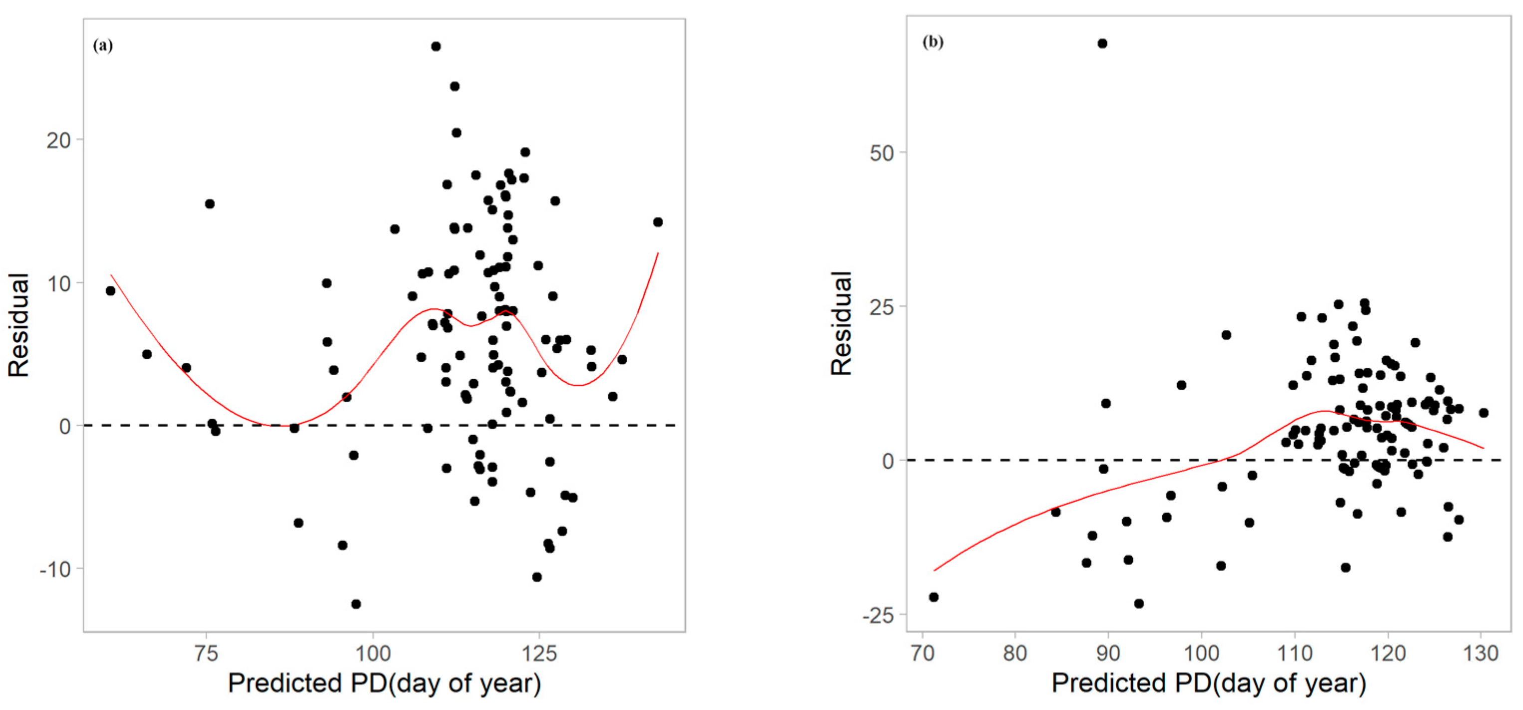
Figure 4 shows the scatter plots of the residual-predicted values of the validation sample points obtained from the two prediction methods, where Figure 4a,b correspond to the environmental similarity method and the multiple linear regression method, respectively. From the distribution of residual values, the range of residuals of the validation sample points obtained from the environmental similarity method was significantly smaller than that of the multiple regression method. From the distribution of the residual-predicted value scatter plot, for the environmental similarity method, it can be seen that the residuals are centered on 0 and scattered, and there are underestimation phenomena (residual values greater than 0) in more validation points, indicating that the choice of environmental variables in the prediction is reasonable, and the results of the prediction are better than those of the multiple linear-regression-based prediction method.

3.2. Predicting Spatial Distribution of Planting Dates

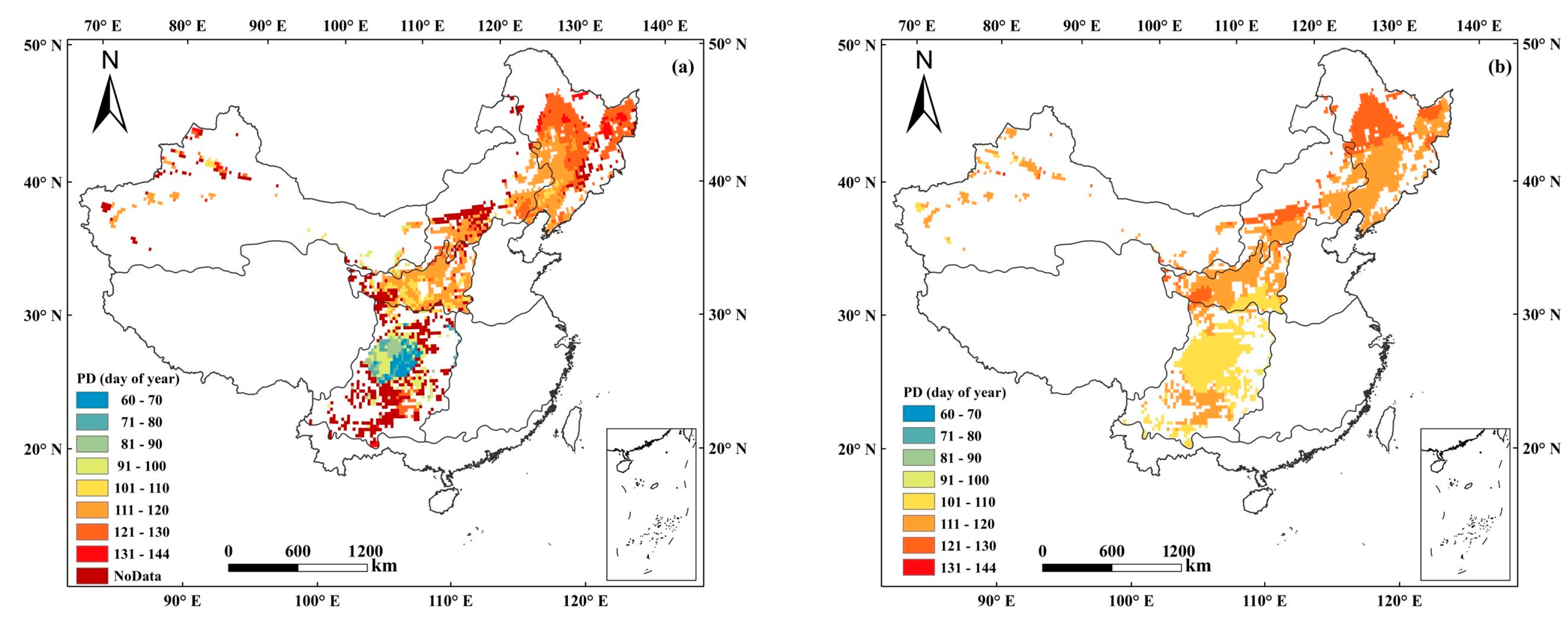
Figure 5a, b illustrates the spatial distributions of predicted spring maize planting dates in 2010 using two different spatial methods. The environmental similarity method predicted planting dates within a range of 60–144 days of the year, while the multiple linear regression method forecasted dates between 97–130 days of the year. Generally, planting dates showed a latitudinal delay, being progressively postponed from southwest to northeast. This trend aligns with considerations of temperature and precipitation, where higher temperatures in the southwest prompt earlier planting compared to the cooler northeast. Notably, the Sichuan Basin exhibited earlier planting due to higher spring temperatures within the basin compared to the adjacent hilly regions. Overall, while both methods depicted consistent spatial planting patterns, the environmental similarity method revealed stronger spatial heterogeneity in planting date variations within each region compared to the multiple linear regression method.
To ensure prediction accuracy using the environmental similarity method, samples were selected based on both environmental similarity and sample point credibility. Consequently, only samples meeting specific conditions were utilized for prediction, resulting in null values in certain regions of the spatial distribution prediction map of planting dates (Figure 5a). These null values primarily appeared in border areas with limited sample representation, indicating a lack of suitable sample points for prediction. Thus, some survey sample sites in the area should be added in a future study. In contrast, the multiple linear regression method utilized the regression model based on available covariates at each point, bypassing sample selection. Consequently, the method does not ensure sample point credibility, potentially affecting the reasonableness of predicted results.

3.3. Uncertainty Analysis of Environmental Similarity-Based Predictions

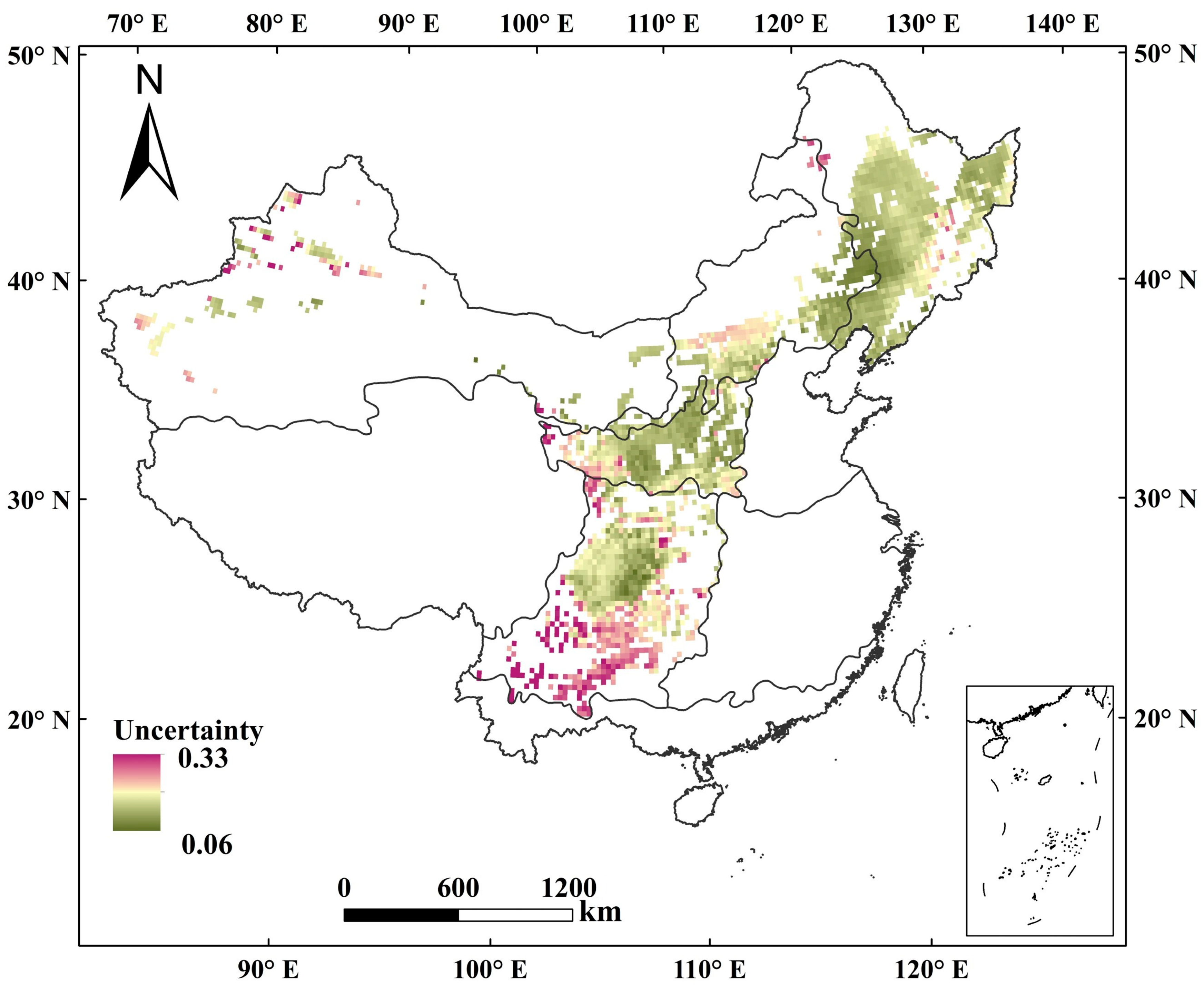
Figure 6 shows the spatial distribution of predicted uncertainty. Overall, the boundaries of each zone exhibited high uncertainty levels. Variations in uncertainty were evident among zones, with lower uncertainty predominantly observed in flatter plains, such as the northeastern plains and the Sichuan Basin in the southwest. Conversely, higher uncertainty prevailed in the northwestern and southwest zones of the Loess Plateau, and along the border of the Inner Mongolia Autonomous Region north of the Great Wall zone. Particularly, the southern region of the southwest zone exhibited the highest uncertainty due to sparse and scattered samples (Figure 1). Limited sample representation in these areas contributed to heightened uncertainty levels overall. Enhancing predictive accuracy necessitates augmenting sample numbers in high-uncertainty regions.

3.4. Comparison of National-Scale and Regional-Scale Prediction

Comparison of the above prediction results shows that the multiple linear regression prediction method was too smooth when predicting over a large area. In contrast, the environmental similarity prediction method could better reflect the spatial heterogeneity at the national scale (the entire Chinese spring maize growing region). Despite variations among growing areas, the natural environmental conditions within each region are relatively homogeneous. Therefore, applying the environmental similarity prediction method to each of the five spring maize zones prompts the query: how do the resulting predictions differ from those made at the national scale?
At the regional scale, covering five cultivation zones, the environmental similarity prediction method was applied, using environmental factor data consistent with the national-scale prediction. The regional scale predictions used samples from 1992 to 2009 as training data, with 2010 samples used as independent validation for each of the five spring maize zones (Table 4).
The validation accuracy of the planting date in five spring maize growing zones is shown in Table 5. The national-scale results were predicted using national data, and then the zonal results are extracted based on each regional scale. The LP zone had the highest accuracy in predicting spring maize planting dates, with RMSE and MAE of 6 and 4 days, respectively, and the proportion of sites with a difference of 5 days between the predicted value and the observed value reached 73.6% (L5 = 73.6%). Conversely, the northeast zone displayed the lowest precision, with an RMSE and MAE of 11 and 10 days, respectively, and 20.8% of sites within 5 days of the observed values (L5 = 20.8%). Overall, the regional-scale predicted accuracy RMSE was between 6 and 10 days, and on the national scale, the RMSE was 10 days. Notably, differences in accuracy between the regional and national scales across planting zones were insignificant, particularly in the NE and IAM zones, where predictions were nearly identical. The LP zone exhibited slightly lower national-scale accuracy compared to regional-scale predictions, while the SW and NW zones showed slightly higher national-scale accuracy compared to regional-scale predictions.
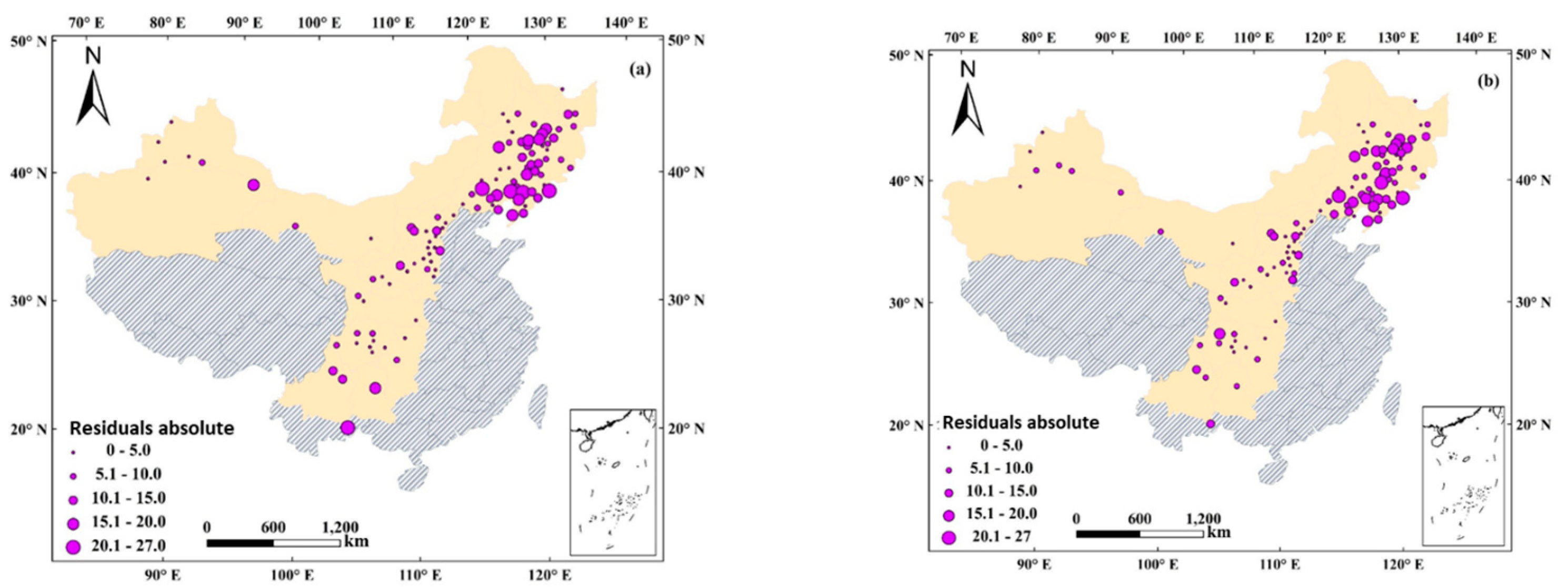
Figure 7 shows the distribution of the absolute residuals for predicted spring maize planting dates in the 2010 validation sample points. Figure 7a represents the residuals at the regional scale, while Figure 7b represents those at the national scale. The spatial representation of sample points with significant differences becomes more evident from these maps. Both regional- and national-scale predictions yielded residuals within 0–27 days. Notably, the NE zone exhibited larger residuals compared to other zones. Overall, national-scale predictions performed better than regional-scale ones. Regional scale predictions, segregated into distinct zones, encountered limitations where sample points at zone boundaries might resemble those in neighboring zones, resulting in fewer predictive sample points and reduced prediction accuracy. Conversely, national-scale predictions, free from boundary constraints, allowed more similar sample points to contribute, thereby enhancing prediction accuracy.

3.5. Advantages and Limitations of the Environmental Similarity Method

Most of the studies used temperature thresholds to predict planting dates [22,24]. The temperature thresholds were set based on field experiments or expert knowledge. When the air temperature or cumulative temperature reaches the set thresholds, the date at this time is the planting date. In addition, considering regional characteristics, rule-based models can incorporate soil temperature, soil moisture, and precipitation to formulate rules for global sowing date prediction [19,31]. Therefore, the SAGE data set [24] of crop calendars was widely used. However, the spatial coverage is relatively limited, and there is only one value for planting date in an administrative zone [31]. Despite the improvements in spatial resolution made by Iizumi et al. [31], their study did not take into account topography and day-length factors. The environmental-similarity-based approach proposed in this study integrates factors such as climate, topography, and sunshine duration (day length), and the predicted planting dates have strong spatial heterogeneity (Figure 5).
This study has some limitations. First, the environmental characterization of planting date is important in the predictive process. Therefore, factors such as soil characteristics, field work capacity, and labor availability should be taken into account in future research. Second, modelling changes in planting dates and the impact on crop yields under future climate change is also an area for future research.

4. Conclusions

This study explored spatial variations in planting dates and environmental data using an environmental similarity prediction method for Chinese spring maize. Comparison of validation accuracy using independent samples indicates superior performance of the environmental similarity method over the multiple linear regression method. In the future, if only the weather conditions are known, the environmental similarity method can be used to predict planting date. Therefore, the environmental similarity method can provide decision-making guidance to farmers in selecting planting dates under the influence of global change. Notably, the environmental similarity method exhibited high accuracy with sampled data and quantified prediction uncertainty at unsampled locations. Employing the environmental similarity method reduces sampling and analytical costs, focusing intensive sampling efforts on under-represented regions. In areas with large differences of planting dates, the precision of the national-scale prediction was better than that of the regional-scale prediction, which sets clear boundaries at the regional boundaries and separates the sample points, so that some sample points that should be used as extrapolations were excluded, which resulted in a slightly lower precision. Future research will involve predicting temporal planting date variations and determining the necessary sampling points to influence prediction outcomes.

Author Contributions

Conceptualization, M.S., A.-X.Z. and T.M.; methodology, M.S. and A.-X.Z.; software, M.S.; validation, X.F.; formal analysis, M.S. and Z.R.; investigation, M.S.; resources, A.-X.Z.; data curation, X.D.; writing—original draft preparation, M.S.; writing—review and editing, A.-X.Z. and T.M.; visualization, X.F.; supervision, T.M.; project administration, Z.R.; funding acquisition, M.S., X.F., and X.D. All authors have read and agreed to the published version of the manuscript.

Funding

This research was funded by the Three Agriculture Nine Party Science and Technology Collaboration Program of Zhejiang Province (Grant No. 2023SNJF041); the Design of Sample Points for Soil Products of the Third Soil Census in Zhejiang Province (Grant No. 2023R28T60D02); and Key Research and Development Program of Zhejiang Province (Grant No. 2020C02023).

Informed Consent Statement

Not applicable

Data Availability Statement

Data are contained within the article.

Conflicts of Interest

The authors declare no conflict of interest.

Abbreviations

PDPlanting date
NENortheast China
IMAInner Mongolia Autonomous Region north of the Great Wall
NWNorthwest China
LPLoess Plateau China
SWSouthwest China
CMAChinese Meteorological Administration
TiMonthly average temperature, the i is the month number
TminiMonthly average minimum temperature, the i is the month number
PiMonthly precipitation, the i is the month number
GDD8Growing degree days above 8 ℃
GDD10Growing degree days above 10 ℃
RARelief amplitude
DEMDigital elevation model
RMSERoot mean square error
MAEMean absolute error
R2Coefficient of determination
LonLongitude
LatLatitude
PCAPrincipal component analysis

References

  1. Foley, J.A.; Ramankutty, N.; Brauman, K.A.; Cassidy, E.S.; Gerber, J.S.; Johnston, M.; Mueller, N.D.; O’Connell, C.; Ray, D.K.; West, P.C.; et al. Solutions for a cultivated planet. Nature 2011, 478, 337–342. [Google Scholar] [CrossRef] [PubMed]
  2. Godfray, H.C.J.; Beddington, J.R.; Crute, I.R.; Haddad, L.; Lawrence, D.; Muir, J.F.; Pretty, J.; Robinson, S.; Thomas, S.M.; Toulmin, C. Food Security: The Challenge of Feeding 9 Billion People. Science 2010, 327, 812–818. [Google Scholar] [CrossRef] [PubMed]
  3. Rosenzweig, C.; Elliott, J.; Deryng, D.; Ruane, A.C.; Müller, C.; Arneth, A.; Boote, K.J.; Folberth, C.; Glotter, M.; Khabarov, N.; et al. Assessing agricultural risks of climate change in the 21st century in a global gridded crop model inter-comparison. Proc. Natl. Acad. Sci. USA 2014, 111, 3268–3273. [Google Scholar] [CrossRef] [PubMed]
  4. Peng, B.; Guan, K.; Chen, M.; Lawrence, D.M.; Pokhrel, Y.; Suyker, A.; Arkebauer, T.; Lu, Y. Improving maize growth processes in the community land model: Implementation and evaluation. Agric. For. Meteorol. 2018, 250–251, 64–89. [Google Scholar] [CrossRef]
  5. FAO. Food and Agriculture Organization of the United Nations (FAO), FAO Statistical Databases. 2022. Available online: http://faostat.fao.org (accessed on 1 December 2023).
  6. National Bureau of Statistics. National Data Bank (In Chinese). 2023. Available online: http://www.stats.gov.cn/ (accessed on 1 December 2023).
  7. Estes, L.D.; Beukes, H.; Bradley, B.A.; Debats, S.R.; Oppenheimer, M.; Ruane, A.C.; Schulze, R.; Tadross, M. Projected climate impacts to South African maize and wheat production in 2055: A comparison of empirical and mechanistic modeling approaches. Glob. Chang. Biol. 2013, 19, 3762–3774. [Google Scholar] [CrossRef]
  8. Lobell, D.B.; Asseng, S. Comparing estimates of climate change impacts from process-based and statistical crop models. Environ. Res. Lett. 2017, 12, 015001. [Google Scholar] [CrossRef]
  9. Craufurd, P.Q.; Wheeler, T.R. Climate change and the flowering time of annual crops. J. Exp. Bot. 2009, 60, 2529–2539. [Google Scholar] [CrossRef] [PubMed]
  10. Siebert, S.; Ewert, F. Spatio-temporal patterns of phenological development in Germany in relation to temperature and day length. Agric. For. Meteorol. 2012, 152, 44–57. [Google Scholar] [CrossRef]
  11. He, L.; Asseng, S.; Zhao, G.; Wu, D.R.; Yang, X.Y.; Zhuang, W.; Jin, N.; Yu, Q. Impacts of recent climate warming, cultivar changes, and crop management on winter wheat phenology across the Loess Plateau of China. Agric. For. Meteorol. 2015, 200, 135–143. [Google Scholar] [CrossRef]
  12. Tao, F.; Zhang, S.; Zhang, Z.; Rötter, R.P. Maize growing duration was prolonged across China in the past three decades under the combined effects of temperature, agronomic management, and cultivar shift. Glob. Chang. Biol. 2014, 20, 3686–3699. [Google Scholar] [CrossRef]
  13. Tao, F.; Zhang, Z.; Xiao, D.; Zhang, S.; Rötter, R.P.; Shi, W.; Liu, Y.; Wang, M.; Liu, F.; Zhang, H. Responses of wheat growth and yield to climate change in different climate zones of China, 1981–2009. Agric. For. Meteorol. 2014, 189–190, 91–104. [Google Scholar] [CrossRef]
  14. van Bussel, L.G.J.; Stehfest, E.; Siebert, S.; Müller, C.; Ewert, F. Simulation of the phenological development of wheat and maize at the global scale. Glob. Ecol. Biogeogr. 2015, 24, 1018–1029. [Google Scholar] [CrossRef]
  15. Koimbori, J.K.; Wang, S.; Pan, J.; Guo, L.; Li, K. Yield Response of Spring Maize under Future Climate and the Effects of Ad-aptation Measures in Northeast China. Plants 2022, 11, 1634. [Google Scholar] [CrossRef] [PubMed]
  16. Kucharik, C.J. Contribution of Planting Date Trends to Increased Maize Yields in the Central United States. Agron. J. 2008, 100, 328. [Google Scholar] [CrossRef]
  17. Twine, T.E.; Kucharik, C.J.; Foley, J.A. Effects of Land Cover Change on the Energy and Water Balance of the Mississippi River Basin. J. Hydrometeorol. 2004, 5, 640–655. [Google Scholar] [CrossRef]
  18. Xu, F.; Wang, B.; He, C.; Liu, D.L.; Feng, P.; Yao, N.; Zhang, R.; Xu, S.; Xue, J.; Feng, H.; et al. Optimizing Sowing Date and Planting Density Can Mitigate the Impacts of Future Climate on Maize Yield: A Case Study in the Guanzhong Plain of China. Agronomy 2021, 11, 1452. [Google Scholar] [CrossRef]
  19. Dobor, L.; Barcza, Z.; Hlásny, T.; Árendás, T.; Spitkó, T.; Fodor, N. Crop planting date matters: Estimation methods and effect on future yields. Agric. For. Meteorol. 2016, 223, 103–115. [Google Scholar] [CrossRef]
  20. Rosenzweig, C.; Parry, M.L. Potential impact of climate change on world food supply. Nature 1994, 367, 133–138. [Google Scholar] [CrossRef]
  21. Tubiello, F.N.; Donatelli, M.; Rosenzweig, C.; O Stockle, C. Effects of climate change and elevated CO2 on cropping systems: Model predictions at two Italian locations. Eur. J. Agron. 2000, 13, 179–189. [Google Scholar] [CrossRef]
  22. Waha, K.; van Bussel, L.G.J.; Müller, C.; Bondeau, A. Climate-driven simulation of global crop sowing dates. Glob. Ecol. Biogeogr. 2011, 21, 247–259. [Google Scholar] [CrossRef]
  23. Deryng, D.; Sacks, W.J.; Barford, C.C.; Ramankutty, N. Simulating the effects of climate and agricultural management practices on global crop yield. Glob. Biogeochem. Cycles 2011, 25. [Google Scholar] [CrossRef]
  24. Sacks, W.J.; Deryng, D.; Foley, J.A.; Ramankutty, N. Crop planting dates: An analysis of global patterns. Glob. Ecol. Biogeogr. 2010, 19, 607–620. [Google Scholar] [CrossRef]
  25. Elliott, J.; Müller, C.; Deryng, D.; Chryssanthacopoulos, J.; Boote, K.J.; Büchner, M.; Foster, I.; Glotter, M.; Heinke, J.; Iizumi, T.; et al. The Global Gridded Crop Model Intercomparison: Data and modeling protocols for Phase 1 (v1.0). Geosci. Model Dev. 2015, 8, 261–277. [Google Scholar] [CrossRef]
  26. Frieler, K.; Lange, S.; Piontek, F.; Reyer, C.P.O.; Schewe, J.; Warszawski, L.; Zhao, F.; Chini, L.; Denvil, S.; Emanuel, K.; et al. Assessing the impacts of 1.5 °C global warming–simulation protocol of the Inter-Sectoral Impact Model Intercomparison Project (ISIMIP2b). Geosci. Model Dev. 2017, 10, 4321–4345. [Google Scholar] [CrossRef]
  27. Ma, Y.P.; Wang, S.L.; Zhang, L. A Preliminary Study on a Regional Growth Simulation Model of Winter Wheat in North China Based on Scaling-up Approach I. Potential Production Level. ACTA Agron. Sin. 2005, 31, 697–705. [Google Scholar]
  28. Liu, Z.; Zan, X.L.; Liu, W.; Li, S.; Zhang, X.; Zhu, D. Filling and comparison of the growth period data of agricultural meteorological stations. Resour. Sci. 2019, 41, 176–184. [Google Scholar]
  29. Yang, Y.; Yang, J.Y.; Li, S.M.; Zhang, X.; Zhu, D. Comparison of spatial interpolation methods for maize growth period. Trans. CSAE 2009, 25, 163–167. [Google Scholar]
  30. Gerstmann, H.; Doktor, D.; Glaser, C.; Möller, M. PHASE: A geostatistical model for the Kriging-based spatial prediction of crop phe-nology using public phenological and climatological observations. Comput. Electron. Agric. 2016, 127, 726–738. [Google Scholar] [CrossRef]
  31. Iizumi, T.; Kim, W.; Nishimori, M. Modeling the Global Sowing and Harvesting Windows of Major Crops Around the Year. Geosci. Model Dev. 2019, 11, 99–112. [Google Scholar] [CrossRef]
  32. Mathison, C.; Deva, C.; Falloon, P.; Challinor, A.J. Estimating sowing and harvest dates based on the Asian summer monsoon. Earth Syst. Dyn. 2018, 9, 563–592. [Google Scholar] [CrossRef]
  33. Parker, P.S.; Shonkwiler, J.S.; Aurbacher, J. Cause and Consequence in Maize Planting Dates in Germany. J. Agron. Crop. Sci. 2016, 203, 227–240. [Google Scholar] [CrossRef]
  34. Sheng, M.; Zhu, A.-X.; Rossiter, D.G.; Liu, J. How Much Are Planting Dates for Maize Affected by the Climate Trend? Lessons for Scenario Analysis Using Land Surface Models. Agronomy 2019, 9, 316. [Google Scholar] [CrossRef]
  35. Gümüşçü, A.; Tenekeci, M.E.; Bilgili, A.V. Estimation of wheat planting date using machine learning algorithms based on available climate data. Sustain. Comput. Inform. Syst. 2019, 28, 100308. [Google Scholar] [CrossRef]
  36. Sheng, M.; Liu, J.; Zhu, A.-X.; Rossiter, D.G.; Zhu, L.; Peng, G. Evaluation of CLM-Crop for maize growth simulation over Northeast China. Ecol. Model. 2018, 377, 26–34. [Google Scholar] [CrossRef]
  37. Zhu, A.-X.; Turner, M. How is the Third Law of Geography different? Ann. GIS 2022, 28, 57–67. [Google Scholar] [CrossRef]
  38. Zhu, A.-X.; Liu, J.; Du, F.; Zhang, S.J.; Qin, C.Z.; Burt, J.; Behrens, T. Scholten. Predictive soil mapping with limited sample data. Eur. J. Soil Sci. 2015, 66, 535–547. [Google Scholar] [CrossRef]
  39. Liu, F.; Rossiter, D.G.; Song, X.-D.; Zhang, G.-L.; Yang, R.-M.; Zhao, Y.-G.; Li, D.-C.; Ju, B. A similarity-based method for three-dimensional prediction of soil organic matter concentration. Geoderma 2016, 263, 254–263. [Google Scholar] [CrossRef]
  40. Zhang, X.-J.; Tang, Q.; Pan, M.; Tang, Y. A Long-Term Land Surface Hydrologic Fluxes and States Dataset for China. J. Hydrometeorol. 2014, 15, 2067–2084. [Google Scholar] [CrossRef]
  41. Gower, J.C. A General Coefficient of Similarity and Some of Its Properties. Biometrics 1971, 27, 857. [Google Scholar] [CrossRef]
  42. Sarbu, C.; Pop, H.F. Principal component analysis versus fuzzy principal component analysis A case study: The quality of daube water (1985–1996). Talanta 2005, 65, 1215–1220. [Google Scholar] [CrossRef]
  43. Shrestha, S.; Kazama, F. Assessment of surface water quality using multivariate statistical techniques: A case study of the Fuji river basin, Japan. Environ. Model. Softw. 2007, 22, 464–475. [Google Scholar] [CrossRef]
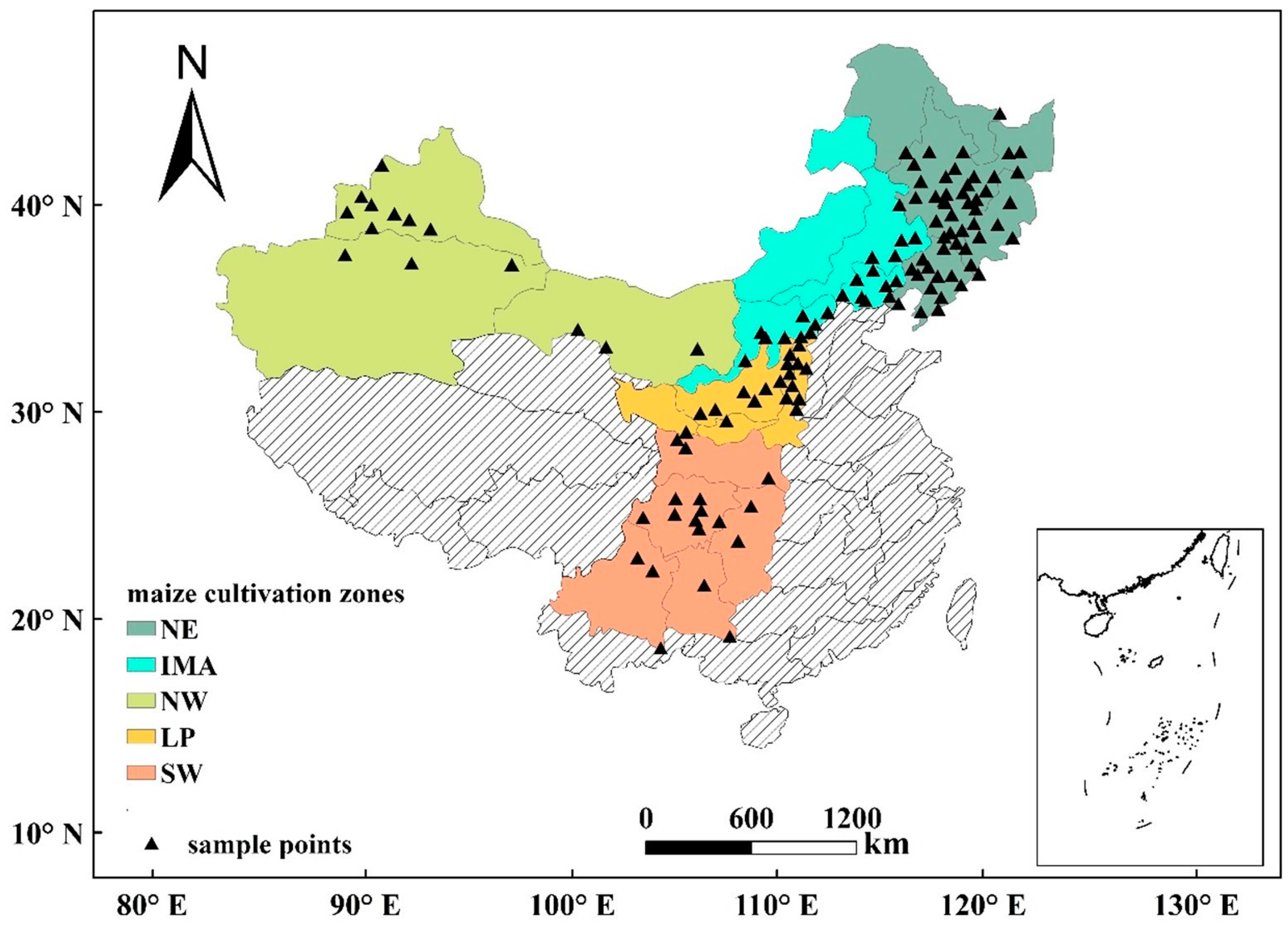
Figure 1. Spring maize cultivation zones of China. The sample points are the locations of agricultural meteorological stations in the cultivation zones.
Agronomy 14 00097 g001
Figure 2. Flowchart of spatially predicting PD based on environmental similarity.
Agronomy 14 00097 g002
Figure 3. Scatterplot of actual versus predicted planting dates using independent validation sample points for spring maize of China: (a) environmental similarity method; (b) multiple line regression method. The dashed line in the plot represents the 1:1 line.
Agronomy 14 00097 g003
Figure 4. The scatter plots of the residual-predicted values of the validation sample points obtained from the two prediction methods: (a) environmental similarity method; (b) multiple line regression method.
Agronomy 14 00097 g004
Figure 5. Predicted spatial distribution of planting dates (day of year) for spring maize in 2010: (a) using environmental similarity method; (b) multiple linear regression method.
Agronomy 14 00097 g005
Figure 6. The spatial distribution of predicted planting dates uncertainty using the environmental similarity method.
Agronomy 14 00097 g006
Figure 7. The distribution of the absolute value of the residuals of the predicted spring maize sowing dates for the 2010 validation sample points: (a) regional-scale prediction; (b) national-scale prediction.
Agronomy 14 00097 g007
Table 1. The summary statistics of planting dates (day of year) of spring maize for the training and validation samples. Min = minimum value. Med = median value. Max = maximum value. SD = standard deviation.
MinMedMeanMaxSD
Training (n = 1404)3911711516715.4
Validation (n = 116)4912312015717.5
Table 2. Eigenvalues, variance contributions, and variable loadings on principal component analysis for spring maize.
VariablesPC1PC2PC3PC4PC5
T20.89−0.21−0.12−0.090.19
Tmin20.91−0.20−0.09−0.090.15
P20.550.180.34−0.08−0.50
T30.92−0.14−0.20−0.090.11
Tmin30.95−0.12−0.12−0.100.06
P30.57−0.120.41−0.10−0.30
T40.910.05−0.21−0.040.05
Tmin40.960.04−0.07−0.080.04
P40.59−0.150.47−0.12−0.12
T50.790.33−0.260.060.06
Tmin50.920.28−0.05−0.010.05
P50.62−0.090.53−0.11−0.14
T60.570.62−0.230.29−0.19
Tmin60.750.560.110.140.01
P60.43−0.080.64−0.260.29
GDD80.920.340.030.040.00
GDD100.900.390.030.06−0.01
Lon−0.440.210.580.150.48
Lat−0.870.350.040.12−0.16
Elevation0.27−0.72−0.51−0.17−0.02
RA0.47−0.530.180.620.00
Slop0.51−0.470.090.660.03
Eigenvalue12.192.552.091.150.84
% of Variance55121054
Cumulative %5567778286
Note: Bold and underlined values indicate strong and moderate loadings, respectively. Ti means the monthly average temperature (i is the month number). Tmini means the monthly average minimum temperature (i is the month number). Pi means the monthly precipitation (i is the month number).
Table 3. Comparison of validation accuracy of independent samples for planting dates in spring maize area of China.
IndictorsMethodology for Spatial Prediction of
Planting Dates
Environmental Similarity MethodMultiple Line Regression Method
RMSE (days)1013
MAE (days)89
R20.640.48
L5(%)37.531.9
Table 4. The summary statistics of spring maize planting dates (day of year) of each five cultivation zones for the training and validation samples. Min = minimum value. Med = median value. Max = maximum value. SD = standard deviation.
Cultivation ZonesType of SamplesNumber of SamplesMinMedMeanMaxSD
NEtraining6511041211221467.6
validation491191311311435.9
IAMtraining2111021181191679.6
validation191131241251427.3
LPtraining216981151141407.0
validation191081161171284.9
SWtraining17939908715721.9
validation1849889115723
NWtraining147881131141389.8
validation11981181181389.8
Table 5. The validation accuracy of independent samples for planting dates in spring maize area of China with regional scale and national scale.
ZonesIndictorsRegional ScaleNational Scale
NERMSE (days)1111
MAE (days)1010
R20.160.16
L5 (%)20.825
IAMRMSE (days)1011
MAE (days)89
R20.040.04
L5 (%)52.636.8
LPRMSE (days)67
MAE (days)45
R20.020.09
L5 (%)73.663.2
SWRMSE (days)108
MAE (days)76
R20.820.85
L5 (%)44.441.2
NWRMSE (days)86
MAE (days)65
R20.580.65
L5 (%)63.644.4
MeanRMSE (days)1010
MAE (days)88
R20.680.64
L5 (%)42.637.5
Disclaimer/Publisher’s Note: The statements, opinions and data contained in all publications are solely those of the individual author(s) and contributor(s) and not of MDPI and/or the editor(s). MDPI and/or the editor(s) disclaim responsibility for any injury to people or property resulting from any ideas, methods, instructions or products referred to in the content.