Combining UAV Multi-Source Remote Sensing Data with CPO-SVR to Estimate Seedling Emergence in Breeding Sunflowers

Abstract

In order to accurately obtain the seedling emergence rate of breeding sunflower and to assess the quality of sowing as well as the merit of sunflower varieties, a method of extracting the sunflower seedling emergence rate using multi-source remote sensing information from unmanned aerial vehicles is proposed. Visible and multispectral images of sunflower seedlings were acquired using a UAV. The thresholding method was used to segment the excess green image of the visible image into vegetation and non-vegetation, to obtain the center point of the vegetation to generate a buffer, and to mask the visible image to achieve weed removal. The components of color models such as the hue–saturation value (HSV), green-relative color space (YCbCr), cyan-magenta-yellow-black (CMYK), and CIELAB color space (L*A*B) models were compared and analyzed. The A component of the L*A*B model was preferred for the optimization of K-means clustering to segment sunflower seedlings and mulch using the genetic algorithm, and the segmentation accuracy was improved by 4.6% compared with the K-means clustering algorithm. All told, 10 geometric features of sunflower seedlings were extracted using segmented images, and 10 vegetation indices and 48 texture features of sunflower seedlings were calculated based on multispectral images. The Pearson’s correlation coefficient method was used to filter the three types of features, and the geometric feature set, the vegetation index set, the texture feature set, and the preferred feature set were constructed. The construction of a sunflower plant number estimation model using the crested porcupine optimizer–support vector machine is proposed and compared with the sunflower plant number estimation models constructed based on decision tree regression, BP neural network, and support vector machine regression. The results show that the accuracy of the model based on the preferred feature set is higher than that of the other three feature sets, indicating that feature screening can improve the accuracy and stability of models; assessed using the CPO-SVR model, the accuracy of the preferred feature set was the highest, with an R² of 0.94, an RMSE of 5.16, and an MAE of 3.03. Compared to the SVR model, the value of the R² is improved by 3.3%, the RMSE decreased by 18.3%, and the MAE decreased by 18.1%. The results of the study can be cost-effective, accurate, and reliable in terms of obtaining the seedling emergence rate of sunflower field breeding.

1. Introduction

Sunflower is one of the five major oilseed crops in China. It is known for its strong barrenness and drought-resistant characteristics, being suitable for growth in areas with long sunshine periods and low rainfall. It has a strong ability to adapt to the ecological environment and is the preferred crop for improving medium and low-salinity land [1]. Therefore, sunflower is suitable for cultivation in the northern and northwestern regions of China, and it has also become an important cash crop with regional characteristics and advantages in China. The seedling emergence rate is an important indicator of seed quality, soil conditions, and sowing management level [2]. A higher seedling emergence rate usually indicates strong seed germination ability, suitable soil and environmental conditions, and proper planting management, while a seedling emergence rate indicates that there may be problems with seed quality, environmental discomfort, pests and diseases, improper sowing, or the influence of other factors. Calculating the seedling emergence rate of the sunflower can help optimize planting density, assess the suitability of soil and environmental conditions, guide rational irrigation and water management, and provide a scientific basis for breeding.

The traditional method of obtaining the sunflower emergence rate mainly relies on manual field sampling and manual estimation, which are time-consuming, laborious, and have low accuracy, and it is difficult to quickly obtain the emergence rate information for large planting areas [3,4]. With the rapid development of UAV remote sensing technology, the calculation of the crop emergence rate has become highly efficient and fast [5,6]. However, in UAV remote sensing images, the presence of weeds and mulch in the field can affect the accuracy of sunflower plant segmentation, which in turn has an impact on the accurate acquisition of the sunflower seedling emergence rate. The commonly used methods for weed removal and mulch segmentation are corrosion and expansion, color features analysis, the threshold method, support vector machine supervised classification, and deep learning segmentation [7], and their advantages and disadvantages are shown in

Table 1. Advantages and disadvantages of different segmentation methods.

Segmentation Method	Advantage	Shortcoming
Expansion, corrosion	Suitable for objects with distinctive morphological features, improving segmentation quality by removing noise and small targets	Poor segmentation on complex backgrounds, difficult to handle overlapping or dense areas.
Color features	Segmentation of objects by analyzing color features (e.g., HSV, lab space), simple calculation, good real-time performance	Sensitive to light conditions and difficult to segment accurately when color features are similar.
The threshold method	Algorithms are simple and easy to implement	Sensitive to light changes and noise, threshold selection needs to be manually adjusted.
Support vector machine-supervised classification	Good classification of multidimensional features	Requires large amounts of labeled data, complex feature selection, and engineering.
Deep learning segmentation	High-precision segmentation of complex scenes	Complex network structure requires a large amount of training data and high computational power, high training cost.

. Li Jinyang removed weed noise by morphological corrosion and expansion operations, and the average error between the number of measured seedlings and the number of estimated seedlings was calculated to be 0.43% using this method [8]. Zhu Sheng et al. performed color feature extraction and principal component analysis on the acquired low altitude visible light images of paddy fields and compared and analyzed them using various machine learning methods such as convolutional neural network and support vector machine. The results showed that the convolutional neural network achieved a classification accuracy of 92.41% for the images [9]. Ning Jifeng and others improved the DeepLabv3+ network by adding learning channel attention and spatial attention features oriented towards the semantic segmentation of the ground cover to achieve the segmentation of the ground cover in the multi-spectral remote sensing image of UAVs [10]. Liang Changjiang et al. analyzed the histograms of RGB and HSV components of ground film, tobacco seedlings, and soil in UAV images and compared the segmentation algorithms such as manual threshold segmentation, iterative threshold segmentation, and big law segmentation. The results show that the iterative threshold segmentation algorithm had the highest recognition rate of 71% [11].

The key to obtaining the seedling emergence rate information lies in the accurate calculation of the number of crop plants in the field, which is usually achieved using UAV remote sensing images, combined with morphological characterization and deep learning methods, for the effective extraction of the number of crop plants [12,13]. Jiang Jiale et al. used remote sensing images acquired by a high-resolution RGB camera carried by a UAV to extract color features and morphological features of cotton at the seedling stage to construct a model for estimating the number of cotton plants. The model constructed based on the morphological parameters (with an R² of 0.9355) had a better fitting effect than that of the model based on the RGB vegetation index (with an R² of 0.9036) [3]. Zheng Xiaolan used spectral information, spatial location, and mathematical morphology information, combined with field survey data, introduced the Hough transform and other mathematical morphology methods to extract the center line of cotton seedling ridges in the field, and constructed a model for estimating the cotton plant using support vector machine regression with R² of 0.9456 [14]. Zhang Hongming et al. constructed a FE-YOLO seedling detection model, and based on the size of the corn seedling and the spatial texture features, constructed a lightweight feature extraction network and fused multiple sensory fields and spatial attention mechanism and the results showed that the model accuracy reached 92% [15]. Liu et al. established three field corn seedling count estimation models as corner point detection model, linear regression model, and deep learning model, respectively, and utilized UAV visible light images taken at different dates and locations to validate the three corn seedling counting models. The model accuracies were 99.78%, 99.9%, and 98.45% for the corn seedling recognition rate, respectively [16]. Oh et al. acquired UAV visible light images of cotton during the seedling stage and used the yolov3 algorithm to separate, localize, and count the cotton, and the RMSE of their model was less than 0.6, and the results showed that the stability of the model was good [17]. However, the deep learning method requires a large number of photos to construct the datasets, and the data preparation and processing are cumbersome.

Currently, there is a wide range of research on plant number extraction for crops grown without mulch, such as cotton, corn, and oilseed rape, but there are still fewer studies on sunflower plant number estimation in complex farmland environments grown with mulch and many weeds. Erosion and swelling methods are commonly used to remove weeds in remote sensing images, but this method is prone to misclassify vulnerable seedlings as weeds and remove them when dealing with large areas of weeds under the mulch. Thresholding and clustering methods are commonly used for the segmentation of mulch and crops, but the selection of segmentation thresholds and clustering centers is more difficult under different light conditions and weeds, resulting in lower image segmentation accuracy. In this paper, we investigated a method to effectively remove weeds and segment the mulch while protecting weak seedlings, and at the same time, optimize the machine learning model to improve the estimation accuracy of the seedling emergence rate of breeding the sunflower to evaluate the merits of sunflower varieties. A method for constructing sunflower buffer zones is proposed to effectively remove weeds and combine color space components with the optimized K-means clustering method for accurate segmentation of mulch and seedlings. A sunflower plant estimation model was constructed based on multiple feature sets and multiple machine learning algorithms, which were trained and validated, and finally, the seedling emergence rate of each sunflower variety was obtained using the optimal estimation model.

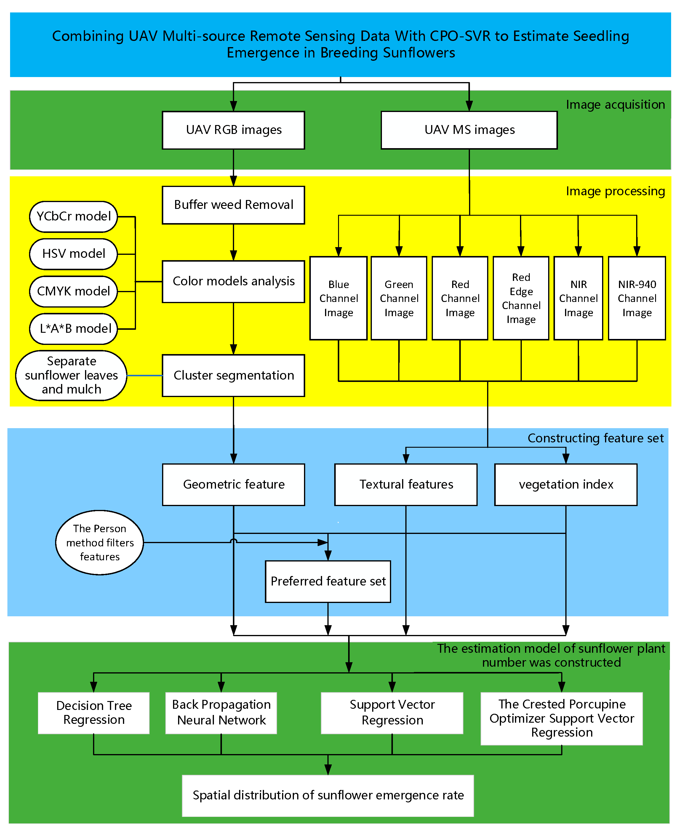
2. Materials and Methods

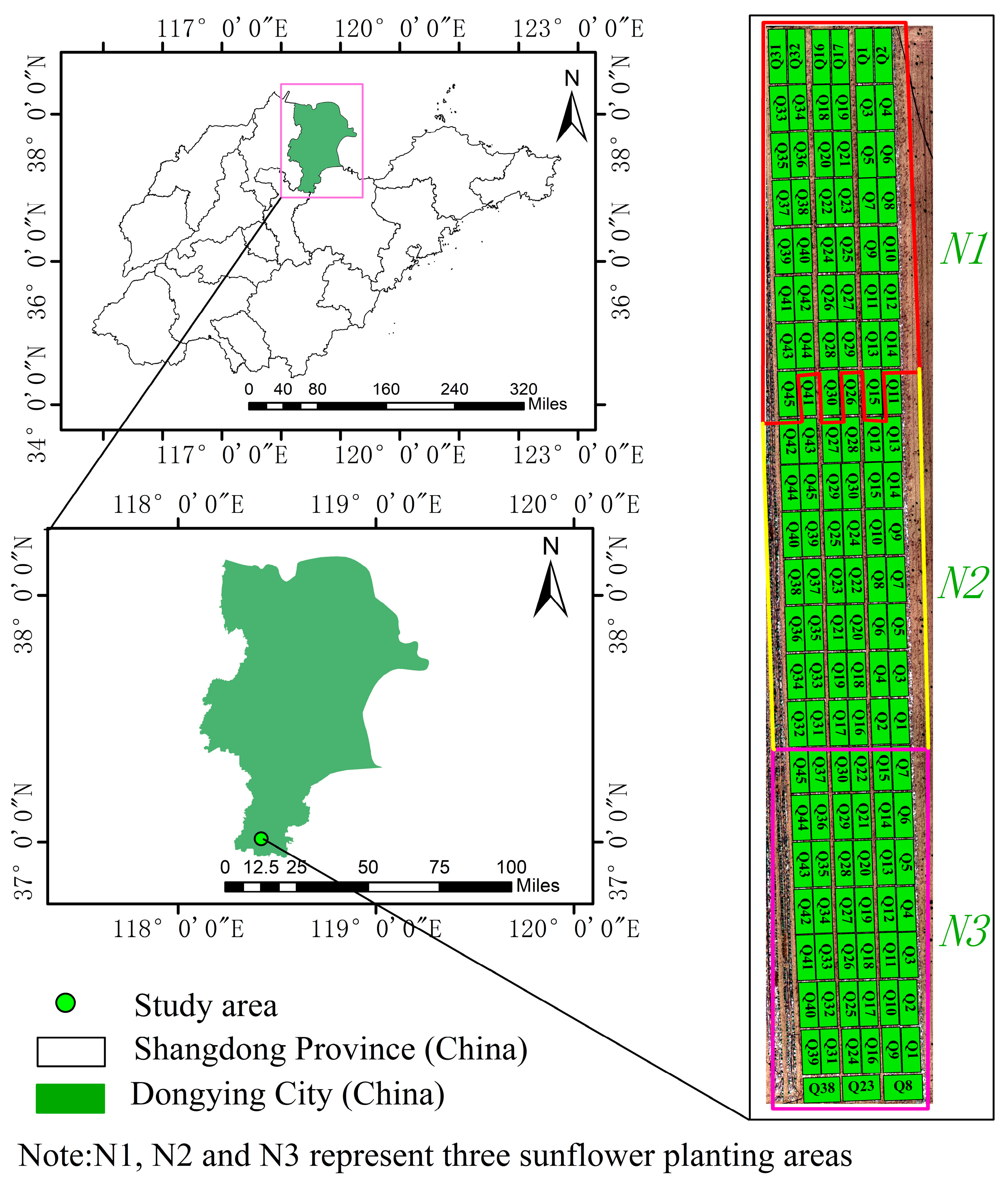
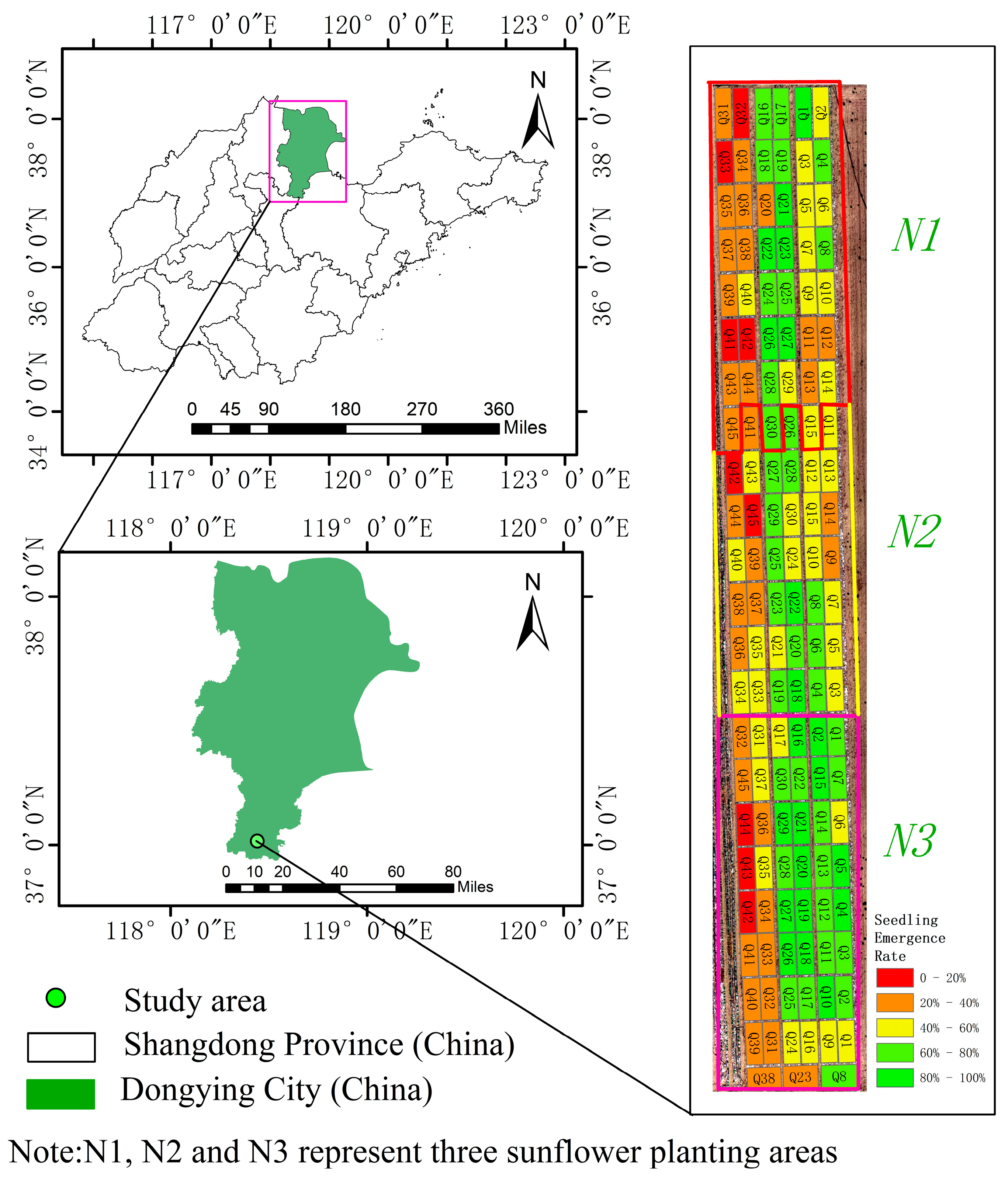
2.1. Overview of the Sunflower Breeding Research Area

The study area is located at the Dongying Base, Shandong Academy of Agricultural Sciences, Guangrao County, Dongying City, Shandong Province, China. The geographical coordinates of Guangrao County are 36°56′~37°21′N, 118°17′~118°57′E, which is located in the warm temperate zone with four distinct seasons. The main sunflower varieties include 30 oil sunflower varieties (such as YK23-1 and YK23-2) and 15 food sunflower varieties (such as JK118 and JK202). A total of 45 sunflower varieties were planted in the whole study area, and each variety was repeatedly planted three times. The planting areas were divided into N1, N2, and N3, and a total of 135 sunflower test plots were set up, as shown in Figure 1. Each experimental plot was planted with 4 rows; the length of the plot was 5 m, the width was 1.8 m, the row spacing was 0.6 m, and the plant spacing was 0.2 m.

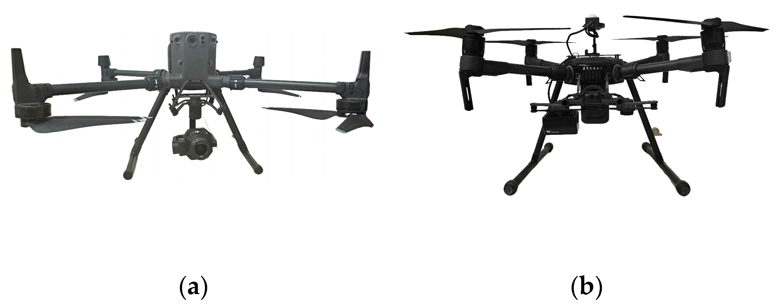
2.2. Sunflower UAV Remote Sensing Image Data Acquisition

The UAV remote sensing image test data were collected on 18 April 2023 (10:00-14:00), as shown in Figure 2 using DJI M300 (DJI, Shenzhen, China) equipped with Zenmuse P1 (DJI, Shenzhen, China) to collect visible remote sensing images, DJI M210 (DJI, Shenzhen, China) equipped with Yusense MS600pro (Yusense, Inc., Qingdao, China) to collect multispectral remote sensing images. The effective pixel value of Zenmuse P1 is 45 megapixels, and the MS600pro multispectral camera (Yusense, Inc., Qingdao, China) has 6 channels, which are blue light (450 mm), green light (555 mm), red light (660 mm), red edge (710 mm), near-infrared 1 (840mm), and near-infrared 2 (940 mm). The weather was clear during the aerial photography; the UAVs flew at an altitude of 30 m, with a heading overlap of 80%, a side overlap of 80%, and a flight speed of 2.3 m/s. The multispectral camera was calibrated using a whiteboard before and after the acquisition. The PIX4Dmapper software (Version 4.4.12, Pix4D S.A., Prilly, Switzerland) was used to stitch and correct the UAV images after acquisition.

It is important to ensure the UAV visible and multispectral images’ precise alignment and to solve the problem of changes in orientation, size, and shape of the captured images due to a variety of factors (light, wind speed, lens distortion, etc.) during the UAV acquisition process, which can lead to deviation, stretching, and distortion between the actual position on the ground and the corresponding position in the images. Therefore, in this paper, ENVI Classic 5.3 software (Version 5.3, Harris Geospatial Solutions, Boulder, CO, USA) was used to perform the calibration of UAV images. The UAV visible and multispectral images were imported into the software, and using the visible image as a baseline, a number of corresponding Ground Control Points (GCPs) were manually selected on the two images, and the alignment was optimized by evaluating the root mean square error (RMSE).

2.3. Research Program

In this experiment, visible images and multispectral images of sunflower seedlings at the 2~4 leaf stage were collected, and a sunflower buffer was constructed to remove weeds from the visible image mask. The color model was used to extract the color components of the masked image, combined with the clustering algorithm to segment the mulch and seedlings to extract the geometric features of the sunflower. The multispectral image was used to calculate a variety of vegetation indices and texture features, and the geometric features, vegetation indices, and texture features were screened by correlation analysis to construct the feature set. A variety of machine regression algorithms were used to construct the estimation model of the number of sunflower plants, obtain the number of sunflower plants that emerged from the study area, and calculate the number of sunflower plants that emerged from the study area. The number of sunflower plants in the study area was obtained, and the sunflower seedling emergence rate was calculated. The technical route is shown in Figure 3.

2.4. Sunflower Visible Image Preprocessing

2.4.1. Weeds Removal

The excess green index mainly reflects the green component of vegetation, is sensitive to changes in the degree of vegetation cover, and can better distinguish between vegetated and non-vegetated areas. A buffer is an area that creates a uniform distance around a particular point, line, or surface, which is called a “graphic buffer” [18].

Figure 4a shows the visible image of the sunflower, revealing that there were large areas of weeds under the mulch and between the ridges. Weeds and the sunflower present similar spectral information in the grayscale image of the vegetation index, as shown in Figure 4b, which affects the sunflower seedling count. To remove the large areas of weeds, the excess green index image was threshold segmented to obtain binarized images of vegetated and non-vegetated areas. The ArcGIS (Version 10.8, Esri, Redlands, CA, USA) was used to convert the binarized image into a point vector file. The sunflower seedlings were connected to adjacent points in the direction of the ridge to generate a centerline vector file. A buffer analysis was performed on the centerline, and the buffer was used to remove the large-area weeds by masking the visible-light image, as shown in Figure 4c. Since the maximum diameter of the outer circle of the sunflower is approximately 0.2 m, the buffer distance is set to 0.2 m, as shown in Figure 4d; this method can effectively remove the weeds with a large area between the ridges and under the mulch.

2.4.2. Choice of Color Model and Segmentation Algorithm

To address the issue of poor segmentation effect caused by difficulty in threshold selection in the threshold segmentation processing method, this paper selects four color space models: hue–saturation value (HSV), green-relative color space (YCbCr), cyan-magenta-yellow-black (CMYK), and CIELAB color space (L*A*B). The K-means clustering algorithm to segment the groundcover and sunflower [19].

The HSV model represents color as three parameters: hue, saturation, and luminance. H represents hue, which is represented by 0 to 360° on the hue ring, counting counterclockwise from red, with red at 0, green at 120°, and blue at 240°. It is applicable to the separation of objects with a specific color, such as a green seedling. S represents the saturation of a color, i.e., the intensity of a color, and is expressed as the proportion of colored components in the hue [20]. In the YCbCr model, Y represents the luminance information, Cb represents the blue chromaticity component, and Cr represents the red chromaticity component. The Cb component is sensitive to the changes in blue and green, and the green plants have distinctive features in the Cb component, which can be distinguished from the background [21]. Compared to the RGB model, YCbCr is better suited for image compression because it effectively separates luminance and chrominance information and reduces data redundancy. The CMYK model consists of C for cyan, M for magenta, Y for yellow, and K for black, with magenta being poor at recognizing green crops and allowing for better separation of background and plant [22]. CMYK works by subtracting color compared to the RGB model and is suitable for converting digital images to physical prints. Black (K) is added to enhance the contrast and depth of the image, reducing inaccuracies caused by mixing colored inks. The three color components in the L*A*B model consist of L for luminance, A for chromaticity from green to red, and B for chromaticity from blue to yellow. Component A is highly sensitive to green and is not affected by light changes, so component A can effectively separate green vegetation from other color backgrounds.

The K-means clustering method is a simple and intuitive algorithm which is easy to understand and implement and has high computational efficiency. The algorithm is a clustering algorithm based on sample sets. Its basic idea is to divide the sample set into k subsets to form k classes. It then divides n samples into k classes, calculates the distance between the samples and their class center, sums all distances, and minimizes them. The goal of K-means clustering is to minimize the loss function, to obtain the optimal division [23]. The distance from a sample to the class center is the square of the Euclidean distance, as shown in Equation (1):

$$d\left(x_i-x_j\right)={‖x_i-x_j‖}^2$$

(1)

where $x_i$ and $x_j$ are two samples in the sample space, and $d\left(x_i-x_j\right)$ is the Euclidean distance between samples $x_i$ and $x_j$.

The sum of the distance between the sample and the center of the class to which it belongs is the loss function, as shown in Equation (2):

$$J\left(C\right)=\sum _{j=1}^k\sum _{i=1}^n{‖x_i-u_j‖}^2$$

(2)

where $k$ represents the number of clusters and $n$ is the total number of samples. $x_i$ denotes the sample belonging to the $j$-th cluster; $u_j$ represents the center of the $j$-th cluster. When the objective function J reaches its minimum, the algorithm converges, and the optimal clustering result is obtained.

However, the results of the K-means clustering algorithm are highly influenced by clustering centers; different clustering centers will lead to different segmentation results and will fall into the local optima. To address this issue, the K-means clustering algorithm is optimized using genetic algorithm (GA). Genetic algorithm can perform a global search in the search space, which avoids local optimal solutions and finds globally optimal clustering results. This method uses Python executed in Visual Studio Code (Version 1.82, Microsoft, Redmond, WA, USA) and obtains the final image segmentation result.

The pixel error rate is a metric used to evaluate how much image segmentation results differ from the true labels and is usually defined as the number of misclassified pixels in a segmented image as a proportion of the actual number of pixels. The value of pixel error rate ranges from 0 to 1, with closer to 0 indicating better segmentation and closer to 1 indicating worse segmentation. The actual pixel count of sunflower seedlings was extracted by defining areas of interest in ENVI software, and the pixel number of sunflower seedlings obtained by the segmentation method was calculated using the Quick Stats function of ENVI software.

$$P={\displaystyle \frac{|N_1-N_2|}{N_1}}\times 100\%$$

(3)

where P is the pixel error rate, N₁ is the actual number of pixels in the sunflower, and N₂ is the number of pixels in the computed sunflower.

2.5. Sunflower Feature Extraction

2.5.1. Sunflower Geometric Feature Extraction

After the split of mulch and sunflower was completed, 10 geometric feature parameters of the sunflower seedling plants were calculated. The correlation between geometric features and the number of plants was obtained by using Pearson’s method, which was used as the basis for the selection of modeling features. This process is shown in

Table 2. Sunflower geometric characterization parameters.

Geometric Feature	Symbolic	Geometric Feature	Symbolic
Area	a1	External Circle Perimeter	a6
Perimeter	a2	The ratio of the area of an external rectangle to its area	a7
External Rectangle Area	a3	The ratio of the perimeter of a rectangle to the perimeter of an externally connected circle	a8
External Rectangle Perimeter	a4	External circle area-to-area ratio	a9
External Circle Area	a5	The ratio of perimeter to circumference of an external circle	a10

.

2.5.2. Sunflower Vegetation Index Extraction

Vegetation indices are combinations of reflectance at certain specific wavelengths in response to plant leaf pigmentation and nutrient status, and data involving two or more bands helps minimize the effects of soil type and light variations. Multi-spectral images can provide more comprehensive and richer spectral information. In this study, six bands of multi-spectral images were selected to calculate 10 vegetation indices commonly used in breeding studies for sunflower seedling estimation. BNDVI reduces the effect of atmospheric scattering in certain conditions and is more effective for assessing the growth status of vegetation. GNDVI is more sensitive to photosynthetic efficiency and biomass of vegetation. NDRE and SIPI are highly sensitive to crop nitrogen and chlorophyll content and are widely used in precision agriculture and crop health monitoring. EVI, through the computation of the three wavelength bands (blue, red, and near-infrared), improves vegetation signal saturation in high-biomass areas. RB-NDVI and GR-NDVI highlight vegetation against other backgrounds (e.g., bare soil or urban buildings). OSAVI enhances the accuracy of vegetation signals using the effect of soil background through an optimization factor. NDVI is extensively used for vegetation growth monitoring, drought monitoring, and ecological research. MCARI detects chlorophyll changes, which is good for crop disease and growth monitoring. Vegetation index grayscale images were generated by the Band Math function in ENVI software (Version 5.3, Harris Geospatial Solutions, Boulder, CO, USA), with the calculation formula shown in

Table 3. List of vegetation index characteristics.

Vegetation Index	Definition	References
Blue Normalized Difference Vegetation Index	$\mathrm{B}\mathrm{N}\mathrm{D}\mathrm{V}\mathrm{I}=\left(\mathrm{N}\mathrm{I}\mathrm{R}-\mathrm{B}\mathrm{L}\mathrm{U}\mathrm{E}\right)/\left(\mathrm{N}\mathrm{I}\mathrm{R}+\mathrm{B}\mathrm{L}\mathrm{U}\mathrm{E}\right)$	[24]
Green Normalized Difference Vegetation Index	$\mathrm{G}\mathrm{N}\mathrm{D}\mathrm{V}\mathrm{I}=\left(\mathrm{N}\mathrm{I}\mathrm{R}-\mathrm{G}\mathrm{R}\mathrm{E}\mathrm{E}\mathrm{N}\right)/\left(\mathrm{N}\mathrm{I}\mathrm{R}+\mathrm{G}\mathrm{R}\mathrm{E}\mathrm{E}\mathrm{N}\right)$	[25]
Normalized Difference Red Edge Index	$\mathrm{N}\mathrm{D}\mathrm{R}\mathrm{E}=\left(\mathrm{N}\mathrm{I}\mathrm{R}-\mathrm{R}\mathrm{E}\right)/\left(\mathrm{N}\mathrm{I}\mathrm{R}+\mathrm{R}\mathrm{E}\right)$	[26]
Enhanced Vegetation Index	$\mathrm{E}\mathrm{V}\mathrm{I}=2.5\left(\mathrm{N}\mathrm{I}\mathrm{R}-\mathrm{R}\mathrm{E}\mathrm{D}\right)/\left(\mathrm{N}\mathrm{I}\mathrm{R}+6\mathrm{R}\mathrm{E}\mathrm{D}-7.5\mathrm{B}\mathrm{L}\mathrm{U}\mathrm{E}+1\right)$	[27]
Red-Blue Normalized Difference Vegetation Index	$\mathrm{R}\mathrm{B}-\mathrm{N}\mathrm{D}\mathrm{V}\mathrm{I}=\mathrm{N}\mathrm{I}\mathrm{R}-\left(\mathrm{R}\mathrm{E}\mathrm{D}+\mathrm{B}\mathrm{L}\mathrm{U}\mathrm{E}\right)/\mathrm{N}\mathrm{I}\mathrm{R}+\left(\mathrm{R}\mathrm{E}\mathrm{D}+\mathrm{B}\mathrm{L}\mathrm{U}\mathrm{E}\right)$	[28]
Red-Green Normalized Difference Vegetation Index	$\mathrm{G}\mathrm{R}-\mathrm{N}\mathrm{D}\mathrm{V}\mathrm{I}=\mathrm{N}\mathrm{I}\mathrm{R}-\left(\mathrm{R}\mathrm{E}\mathrm{D}-\mathrm{G}\mathrm{R}\mathrm{E}\mathrm{E}\mathrm{N}\right)/\mathrm{N}\mathrm{I}\mathrm{R}-\left(\mathrm{R}\mathrm{E}\mathrm{D}+\mathrm{G}\mathrm{R}\mathrm{E}\mathrm{E}\mathrm{N}\right)$	[29]
Optimization of Soil-Adjusted Vegetation Index	$\mathrm{O}\mathrm{S}\mathrm{A}\mathrm{V}\mathrm{I}=\left(\mathrm{N}\mathrm{I}\mathrm{R}-\mathrm{R}\mathrm{E}\mathrm{D}\right)/\left(\mathrm{N}\mathrm{I}\mathrm{R}+\mathrm{R}\mathrm{E}\mathrm{D}+0.16\right)$	[30]
Normalized Difference Vegetation Index	$\mathrm{N}\mathrm{D}\mathrm{V}\mathrm{I}=\left(\mathrm{N}\mathrm{I}\mathrm{R}-\mathrm{R}\mathrm{E}\mathrm{D}\right)/(\mathrm{N}\mathrm{I}\mathrm{R}+\mathrm{R}\mathrm{E}\mathrm{D})$	[31]
Modified Chlorophyll Absorption Reflectance Index	$\mathrm{M}\mathrm{C}\mathrm{A}\mathrm{R}\mathrm{I}=\left[\left(\mathrm{R}\mathrm{E}-\mathrm{R}\right)-0.2\times \left(\mathrm{R}\mathrm{E}-\mathrm{G}\right)\right]\times \left(\mathrm{R}\mathrm{E}/\mathrm{R}\right)$	[32]
Structure-Independent Pigment Index	$\mathrm{S}\mathrm{I}\mathrm{P}\mathrm{I}=\left(\mathrm{N}\mathrm{I}\mathrm{R}-\mathrm{B}\right)/\left(\mathrm{N}\mathrm{I}\mathrm{R}-\mathrm{R}\right)$	[33]

.

2.5.3. Sunflower Texture Feature Extraction

For vegetation monitoring and agricultural research, there is a close relationship between texture characteristics and the number of plants. Dense vegetation typically exhibits more complex texture characteristics, such as higher textural roughness. Sparse vegetation, on the other hand, exhibits simple texture features and higher uniformity. In this paper, we use the Gray-Level Co-occurrence Matrix (GLCM) to calculate the texture features of six channels of multi-spectral images, including mean (MEA), variance (VAR), homogeneity (HOM), contrast (CON), heterogeneity (HOM), and contrast (CON), dissimilarity (DIS), entropy (ENT), second moment (SEM), and correlation (COR). Mean represents the average pixel gray levels in an image, reflecting the overall brightness of the image, with mulch film being brighter in light relative to plant leaves. Variance measures the degree of dispersion in the distribution of pixel gray levels in an image. Symmetry reflects the homogeneity of the texture. Contrast indicates the degree of variation between the gray levels in an image. Dissimilarity measures the degree of difference in the gray levels between different regions of an image, i.e., the degree to which neighboring regions are of the image. Entropy indicates the uncertainty or information content of the image, with higher values indicating a more complex image texture. Second-order moments measure the frequency or probability of occurrence of pixel pairs in an image; correlation measures the linear relationship between the gray values of pixel pairs in an image. The surface of the leaf has rich texture and color variations, while the surface of the mulch is relatively smooth and uniform, so the mean of the mulch is larger than that of the leaf, the homogeneity of the mulch is higher than that of the leaf, the variance of the leaf is higher than that of the mulch, the contrast of the leaf is higher than that of the mulch, the phase anisotropy of the leaf is higher than that of the mulch, the entropy of the leaf is higher than that of the mulch, the second moment of the mulch is higher than that of the leaf. The correlation of the mulch is higher than that of the leaf. The correlation of ground film is higher than the correlation of leaves.

2.6. Pearson’s Correlation Analysis

In statistics, Pearson’s correlation analysis is based on Pearson’s correlation coefficient (PCC) to measure the correlation between two variables X and Y with a value between −1 and 1. The greater the absolute value of the correlation coefficient, the stronger the correlation between the two. This method is widely used for variable screening and can effectively reduce redundant variables. Assuming that there are n different samples, Pearson’s phase relation value (r) can be calculated by Equation (4):

$$r={\displaystyle \frac{{\sum }_{i=1}^n\left(X_i-\overline{X}\right)\left(Y_i-\overline{Y}\right)}{\sqrt{{\sum }_{i=1}^n{\left(X_i-\overline{X}\right)}^2}\sqrt{{\sum }_{i=1}^n{\left(Y_i-\overline{Y}\right)}^2}}}$$

(4)

where $X_i$ and $Y_i$ are the measured values of the two input variables, and $\overline{X}$ and $\overline{Y}$ are their average values. In this study, Pearson’s correlation analysis was completed by data-processing software Origin (Version 2023, OriginLab Corporation, Northampton, MA, USA).

2.7. Construction of a Model for Estimating the Number of Sunflower Plants

In this paper, four feature sets were established with the vegetation index, texture features, and geometric features of the sunflower seedling stage. These feature sets include the geometric feature set, vegetation index set, texture feature set, and preferred feature set. The number of plants in the sample points was used as the output to construct the plant estimation model. A total of 350 sample points were selected from UAV remote sensing images to obtain feature data, and the training and test sets were created with a 2:1 ratio.

• Decision tree regression (DTR) is a recursive process in which the algorithm begins at the root node and selects the optimal feature to split the dataset into two subsets. This selection is typically based on some partitioning criterion, such as minimizing the squared error, such that the squared error of the partitioned subset is minimized. The process is repeated recursively on each subset until the stopping condition is met. The decision tree regression algorithm was implemented using the Scikit-learn (Version 1.3.0) package in Python and executed in Visual Studio Code software (Version 1.82, Microsoft, Redmond, WA, USA). The parameters of the algorithm were set as follows: max_depth is 3.
• The back propagation neural network (BPNN) is an artificial neural network model based on the backpropagation algorithm, adapting to different data distributions and features, with strong adaptive ability, used to solve regression problems. BPNN consists of input, hidden, and output layers; it learns complex relationships between input data and predicts output values through connections between neurons across multiple layers. It optimizes the model fit by continuously adjusting connection weights and using gradient descent to minimize the prediction error. The BP Neural Network Regression algorithm was implemented using the TensorFlow (Version 2.16.1) library in Python and executed in Visual Studio Code (Version 1.82, Microsoft, Redmond, WA, USA). The parameters of the algorithm were set as follows: activation is relu, the loss is mean_squared_error, the optimizer is adam, epochs is 300, and the batch_size is 10.
• The support vector regression (SVR) can handle nonlinear relationships through the kernel function, mapping the original linearly indivisible data into the high-dimensional space, realizing the linear separability, and making the model more flexible. It is applicable to various types of data so that the effect of the data processing in high-dimensional space is significant. SVM’s objective function is a convex function; there are no local minima, which makes the training process more reliable. This ensures the stability of model training and convergence, providing a reliable foundation for practical applications. The SVM algorithm was implemented using the Scikit-learn (Version 1.3.0) package in Python and executed in Visual Studio Code (Version 1.82, Microsoft, Redmond, WA, USA). The parameters of the algorithm were set as follows: kernel is rbf, C parameter is 15.0, and gamma is 0.5.
• The crested porcupine optimizer support vector regression (CPO-SVR) algorithm efficiently searches the hyperparameter space, including the kernel function and regularization parameters. The global search capability makes finding the optimal hyperparameters in support vector regression faster and more reliable. In SVR models, there are often complex nonlinear relationships, and the CPO algorithm helps the model fit the data better, capture the complex relationships between features, and improve the predictive performance of the model [34]. The CPO-SVR algorithm was implemented using the Scikit-learn (Version 1.3.0) package in Python and executed in Visual Studio Code (Version 1.82, Microsoft, Redmond, WA, USA). The parameters of the algorithm were set as follows: pop_size is 10, dim is 2, and the kernel is rbf.

2.8. Evaluation of the Estimation Accuracy of Sunflower Plant Number Models

The coefficient of determination (R²), root mean square error (RMSE), and mean absolute error (MAE) are used to evaluate the model, and the value of R² ranges from 0 to 1. A higher value of R² indicates that the model explains the variability of the dependent variable better, meaning the model fits well. R² ranges from 0 to 1; a higher value of R² indicates that the model can explain the variability of the dependent variable better, meaning the model has a better fit. RMSE assesses the difference between the predicted and actual observed values, a smaller value of RMSE indicates that the model has a better fit. MAE is a commonly used goodness-of-fit metric to assess the difference between the predicted and the actual values. A smaller MAE indicates a better fit. The calculation formulas are as follows:

$$R^2={\displaystyle \frac{{\sum }_i\left(\widehat{y_i}-\overline{y}\right)}{{\sum }_i\left(y_i-\overline{y}\right)}}$$

(5)

$$RMSE=\sqrt{{\displaystyle \frac{{\sum }_i{\left(\widehat{y_i}-y_i\right)}^2}{n}}}$$

(6)

$$MAE={\displaystyle \frac{{\sum }_i\left|\widehat{y_i}-y_i\right|}{n}}$$

(7)

where n denotes the total number of samples; $\widehat{y_i}$ denotes the estimated number of sunflower plants; $y_i$ denotes the number of sunflower plants measurements; and $\overline{y}$ denotes the mean of the number of sunflower plants measurements.

3. Results

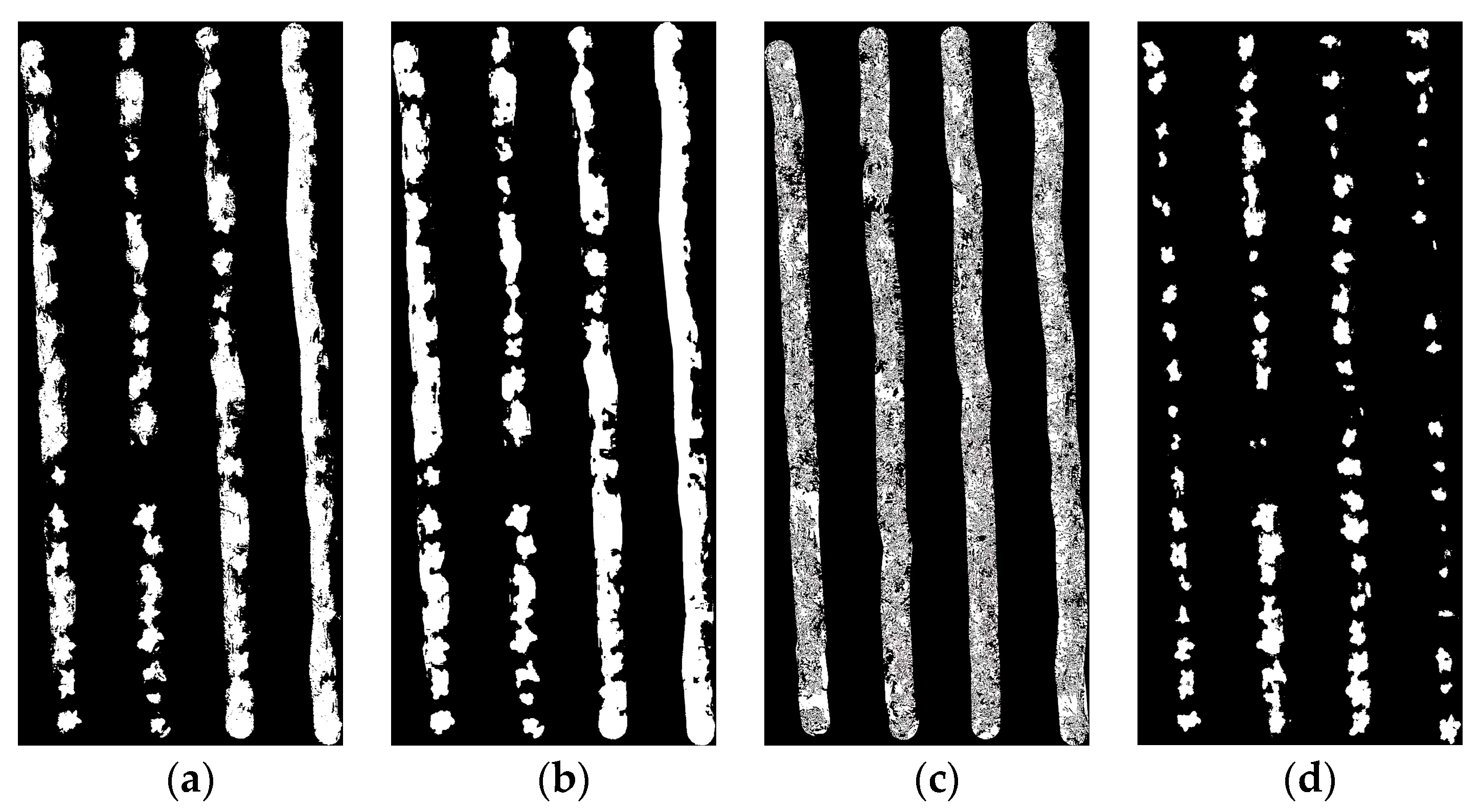
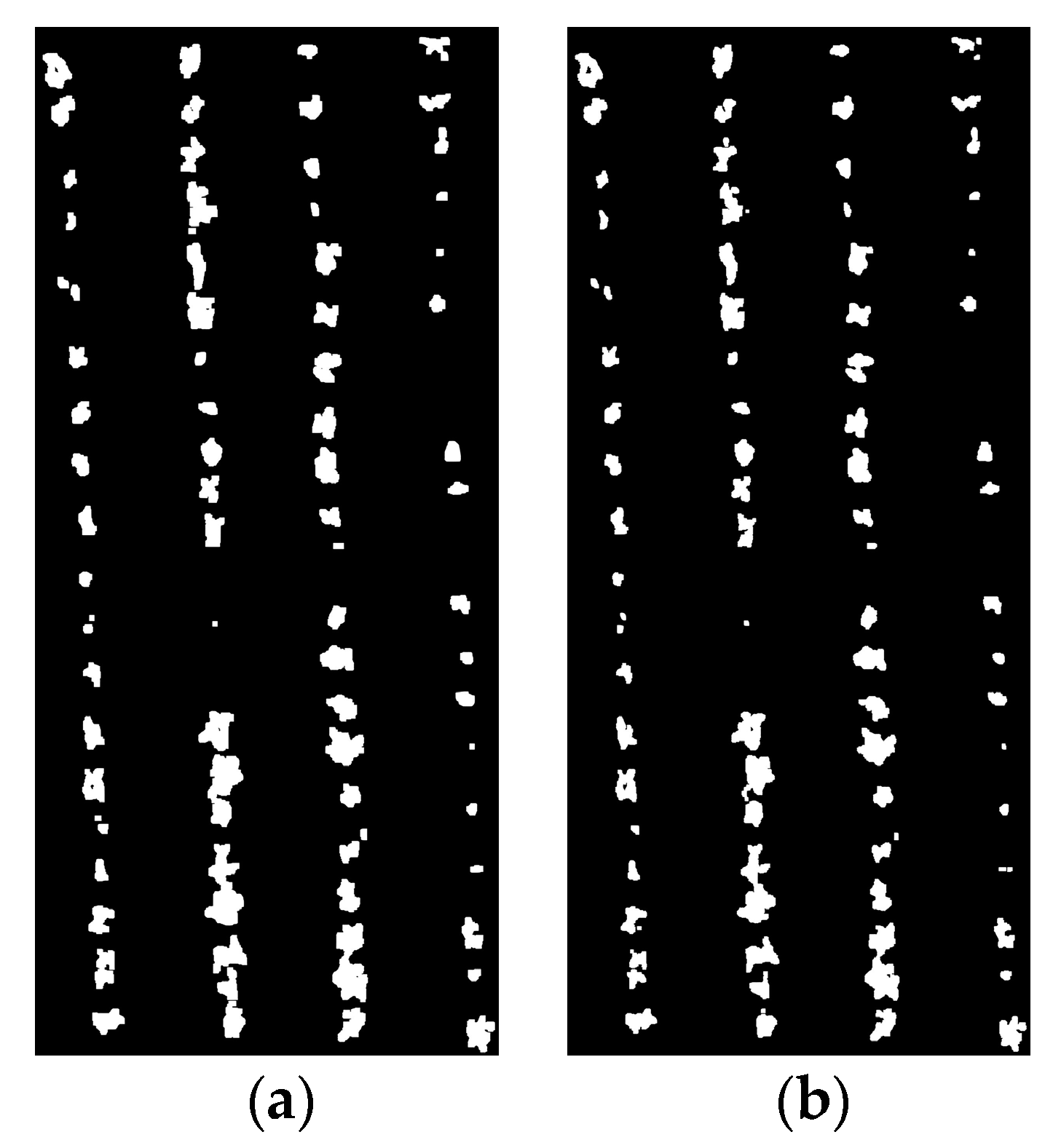
3.1. Segmentation of Sunflower Seedlings and Mulch Film

In this study, the S component in the HSV model, the Cb component in the YCbCr model, the M component in the CMYK model, and the A component in the L*A*B model were extracted. The K-means clustering method is used to segment the image of four color model components of the visible image after masking.

As shown in Figure 5, the A component of L*A*B has the best segmentation effect using the K-means clustering algorithm, and the other three segmentation performances are poor and cannot separate the seedlings from the ground film. A component of L*A*B was selected to segment the sunflower seedlings from the ground film. To further improve the segmentation accuracy, K-means clustering was optimized using a genetic algorithm, and the pixel error rate was calculated for comparative analysis.

In order to make the contour of sunflower leaves smoother, corrosion and expansion are used to remove the noise around the leaves. The denoising result after segmentation is shown in Figure 6, and the number of pixel points of sunflower seedlings in the images of Figure 6a and Figure 6b is 57,414 and 54,950, respectively, and the actual number of sunflower pixel points is 53558. The segmentation accuracy of the K-means clustering algorithm and GA-K-means clustering algorithm for the A-component image of the L*A*B model is calculated, and the pixel error rates are 7.2% and 2.6%. Thus, the optimization of the K-means clustering algorithm using the genetic algorithm can improve the accuracy of segmentation of mulch and seedlings by 4.6%.

3.2. Sunflower Characterization Screening

Pearson’s method is applicable to a variety of data types and feature distributions. It effectively identifies the linear relationship between features. When there is a clear linear correlation in the dataset, it can more accurately filter out the features with a strong correlation.

In order to solve the redundancy of features, this study uses Pearson’s method to calculate the correlation between geometric features, vegetation indices, texture features, and the number of sunflower plants, respectively, as shown in

Table 4. Correlation between characteristics and number of sunflower plants.

Geometric Feature	Correlation	Vegetation Index	Correlation	Texture Features	Correlation
a1	0.844 **	BNDVI	0.824 **	Red-HOM	0.815 **
a2	0.940 **	GRNDVI	0.088	Red-SEM	0.813 **
a3	0.854 **	NRI	−0.752 **	Red-COR	0.821 **
a4	0.942 **	MCARI	0.811 **	Blue-HOM	0.820 **
a5	0.079	NDVI	0.825 **	Blue-SEM	0.817 **
a6	0.932 **	EVI	0.811 **	Blue-COR	0.831 **
a7	0.0255	NDRE	0.827 **	Green-HOM	0.817 **
a8	−0.266 **	OSAVI	0.819 **	Green--SEM	0.819 **
a9	0.006	GNDVI	0.820 **	Redge-HOM	0.816 **
a10	−0.271 **	SIPI	0.827 **	Redge-SEM	0.814 **

Note: ** at the 0.01 level (two-tailed), the correlation is significant.

.

As shown in Table 4, the correlation between geometric features a1, a2, a3, a4, and a6, and the number of plants was greater than 0.8, with the correlation between a2, a4, and a6 and the number of plants being 0.940, 0.942, and 0.932, respectively.The correlation between the other features and the number of plants was less than 0.3, indicating a lower correlation. The characteristics of vegetation indices are shown in Table 4. The correlation between GRNDVI and the number of plants was less than 0.2, and a negative correlation between NRI and the number of plants was shown, while the absolute value of the correlation between the other vegetation indices and the number of plants was greater than 0.7. The correlation between SIPI, NDRE, and NDVI and the number of plants was 0.827, 0.827, and 0.825, respectively, indicating a strong correlation.

In this study, the correlation between 48 kinds of texture features and the number of plants was calculated. To ensure that the number of features in the feature set was the same, the top 10 texture features with correlation were selected. The correlation between 10 kinds of texture features and the number of plants was greater than 0.8. Among these, the correlation between Blue-COR and the number of plants was the highest at 0.831. The geometric features, vegetation indices, and texture features were comprehensively analyzed, and the top 10 features with a higher correlation with the number of plants were selected. The geometric features, including a1, a2, a3, a4, and a6; the vegetation indices, including NDVI, SIPI, and NDRE; and the texture features, including Red-COR and Blue-COR, were analyzed together to select the top 10 features with higher correlation with the number of plants to form the preferred feature set.

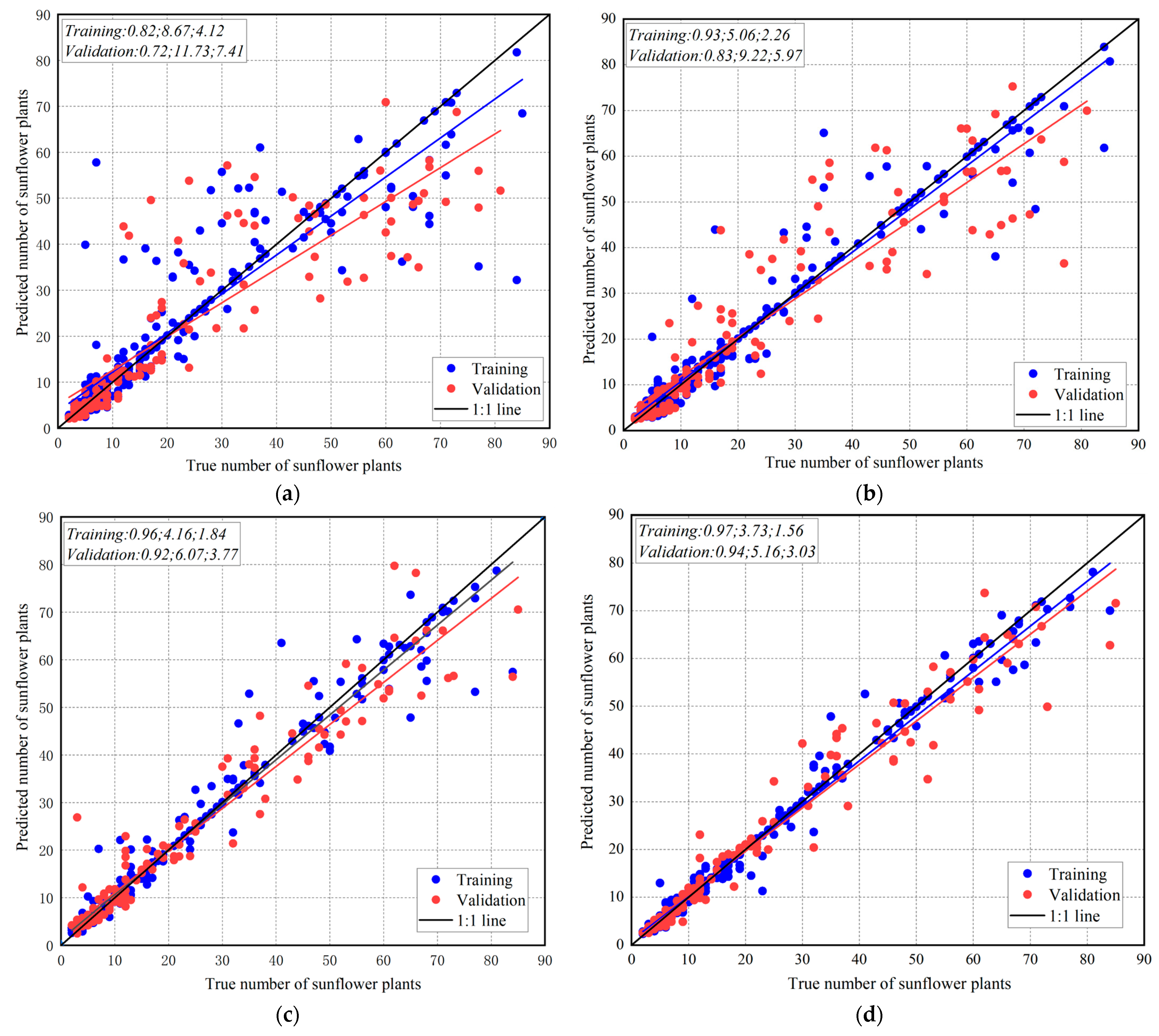
3.3. Analysis of the Results of the Model for Estimating the Number of Sunflower Plants

In this study, four feature sets were used as input variables to estimate the number of sunflower plants using DTR, BPNN, SVM, and CPO-SVR. Feature set A is the vegetation index set containing 10 vegetation indices, and feature set B is the geometric feature set containing 10 geometric features. Feature set C is the texture feature set containing 10 texture features, and feature set D is the preferred feature set, which contains a total of 10 features of a1, a2, a3, a4, a6, NDVI, SIPI, NDRE, Red-COR, and Blue-COR.

As shown in

Table 5. Evaluation of a model for estimating the number of sunflower plants.

Model	Feature Set	Training			Validation
		R2	RMSE	MAE	R2	RMSE	MAE
DTR	Texture Feature Set (A)	0.73	10.60	6.30	0.71	11.90	7.52
	Vegetation Index Set (B)	0.76	10.33	6.48	0.72	11.47	7.05
	Geometric Feature Set (C)	0.91	6.43	4.16	0.84	7.93	4.93
	Preferred Feature Set (D)	0.92	5.97	3.92	0.88	7.60	4.97
BPNN	Texture Feature Set (A)	0.67	11.70	7.69	0.66	13.03	8.19
	Vegetation Index Set (B)	0.70	11.13	6.95	0.70	12.27	7.12
	Geometric Feature Set (C)	0.89	6.84	4.52	0.89	7.38	4.55
	Preferred Feature Set (D)	0.89	6.66	4.29	0.89	7.36	4.45
SVR	Texture Feature Set (A)	0.71	11.51	6.95	0.70	11.33	6.97
	Vegetation Index Set (B)	0.74	10.09	5.81	0.73	12.09	7.55
	Geometric Feature Set (C)	0.93	5.43	3.27	0.90	6.11	3.69
	Preferred Feature Set (D)	0.93	5.41	3.24	0.91	6.32	3.70
CPO-SVR	Texture Feature Set (A)	0.82	8.67	4.12	0.72	11.73	7.41
	Vegetation Index Set (B)	0.93	5.06	2.26	0.83	9.22	5.97
	Geometric Feature Set (C)	0.96	4.16	1.84	0.92	6.07	3.77
	Preferred Feature Set (D)	0.97	3.73	1.56	0.94	5.16	3.03

, when comparing the effects of different feature sets on model accuracy, feature set D was superior to the other three feature sets, while the plant number estimation model constructed with feature set A as the input variable had the lowest accuracy. In SVR, the R² value of the plant number estimation model accuracy constructed with feature sets A and D as input variables differed by 0.21, the RMSE value differed by 5.01, and the MAE value differed by 3.27. When comparing the effects of different algorithms on the model accuracy, the accuracy of the SVR model was better than that of the other two algorithms. Using feature set D as the input variable, the R² value of SVR increased by 0.03, the RMSE value decreased by 1.28, and the MAE value decreased by 1.27, compared to DTR, and the model accuracy is greatly improved. The above study shows that the model accuracy of the three machine learning algorithms with feature set D as the input variable is better than that of feature sets A, B, and C as the input variable, respectively, indicating that the combination of features can improve the model stability and estimation accuracy.

To further improve the accuracy and stability of the model, sunflower plants were estimated using CPO-SVR. The CPO-SVR algorithm had the lowest accuracy for the plant estimation model with the feature set A as the input variable, which had an R² of 0.72. In contrast, the R² of the models with C and D as the input variables were both greater than 0.9. The model using feature set D as the input variable achieved the highest accuracy, with an R² of 0.94, an RMSE of 5.16, and an MAE of 3.03. This represents an increase in the value of 3.3%, a decrease in the RMSE by 18.3%, and a decrease in the MAE by 18.1% compared to the SVR model. As shown in Figure 7, the regression of true versus predicted strain values for the CPO-SVR model is plotted.

3.4. Analysis of Seedling Emergence of Sunflower Varieties

Figure 8 shows that sunflower varieties, including Q31~Q45, had poorer seedling emergence than the other varieties, and the varieties with better seedling emergence included Q20, Q22, and Q27. Figure 9 shows the spatial distribution of the sunflower emergence rate in the sunflower breeding plots, showing that the sunflower emergence rate in the N3 planting area was higher than in the other two areas. Overall, the number of sunflower plots with more than 80% emergence was 21, with N3-Q27 plots having the highest emergence rate of 100% and N3-Q42 plots having the lowest emergence rate of 5.8%.

4. Discussion

In order to improve sunflower seedling emergence, field mulching is performed after sowing, leading to a large number of weeds growing under the mulch between the ridges. In order to eliminate the effect of weeds on the statistics of crop emergence rate, Dai et al. [5] found that using morphological operations to remove weeds is ineffective for large weed areas, and there is the misoperation of removing cotton seedlings as weeds, which affects the calculation of emergence rate. In this study, the buffer zone method is used to remove weeds, which solves the problem of morphological feature changes caused by corrosion and expansion denoising treatment, resulting in more accurate denoising. Zhao et al. [18] also confirmed that the buffer zone method can effectively remove weeds in large inter-row areas.

In order to better identify sunflower leaves and achieve the segmentation of leaves and mulch, first, the sunflower visible image is color transformed; Liu Shuai Bing [16] and Xu Xin [35] et al. showed that the visible image can be more effective in identifying crop leaves by color transformation. This study shows that the A component in the L*A*B model performs best in recognizing sunflower leaves. This is because the L*A*B color space simulates the human eye’s perception of color, and green is typically easier to distinguish in the visual system, especially in low-saturation environments. Since the sunflower seedlings in the UAV images were weak and the leaves were less saturated with green, the A component recognized the leaves more effectively, consistent with the findings of Niu Yaxiao et al. [19].

In selecting the segmentation algorithm, threshold segmentation requires choosing a threshold value based on experience, and the different selection of the threshold value will lead to poor segmentation performance. Zhang Xinliang [36] et al. research confirms this viewpoint and concludes that the K-means clustering algorithm is better than threshold segmentation. Therefore, in this study, the visible image of sunflower was transformed into L*A*B color space to extract the A component, and a genetic algorithm was used to optimize the K-means clustering algorithm to realize the segmentation of mulch and sunflower, compared to the K-means clustering algorithm, which effectively overcame the problem of the weak global search ability and sensitivity of the center of clustering of the K-means clustering algorithm, which the segmentation accuracy improved by 4.6%. Li Kai et al. [23] studied the optimization of the K-means clustering algorithm using particle swarm algorithm to segment cotton leaves and background, and the segmentation accuracy was improved by 5.41% compared to the traditional K-means clustering algorithm. Both the genetic algorithm and particle swarm algorithm are population-based global optimization algorithms. They iteratively update individuals or particles in the population by using a fitness function to evaluate the quality of the solution and include randomness to avoid falling into a local optimum.

In this study, we established four feature sets, geometric features, vegetation indices, texture features, and preferred features, and constructed a sunflower plant number estimation model using DTR, BPNN, SVR, and CPO-SVR machine learning algorithms. We calculated the correlation between each feature and the number of plants. To ensure that the number of features in the established feature sets is the same, the number of features in each feature set is 10, which was used to compare the effect of the feature sets on the estimation accuracy of the model. Regarding the correlation between the features, it has less impact on the performance of the selected machine learning algorithm used to build the model. This is because the SVR model primarily focuses on the support vectors, and even if there are highly correlated features, the model mainly relies on the support vectors for prediction, thereby reducing the impact of feature redundancy. Meanwhile, we used the radial basis function (RBF) kernel to map the input features into a high-dimensional space. In this space, linear correlations between features are weakened or eliminated. The segmentation process of the DTR model involves selecting an optimal feature at each node for segmentation. Even if two features are highly correlated, the decision tree selects one for segmentation based on the segmentation criterion (mean square error) without relying on multiple correlated features simultaneously. This selection process makes the correlation between features have less impact on the model performance. During BPNN training, linear correlations between features are converted into a nonlinear relationship by the activation function (ReLU), which helps reduce the negative impact of feature correlation on the model. Additionally, the backpropagation algorithm adjusts the weights in the network by calculating the error gradient. Even if the features are correlated, the BP neural network, by continuously adjusting the weights, eventually reduces the effect of redundant features and, thus, improves the generalization ability of the model. Therefore, feature correlation has minimal effect on model accuracy.

In this study, four feature sets combined with four machine learning algorithms were used to construct a model for estimating the number of sunflower plants. The results show that among the four feature sets, the model accuracy of the preferred feature set is higher than that of the other three feature sets, followed by the geometric feature set, while the texture feature set has the lowest model accuracy. The reason for this is that the preferred feature set retains the features that have the closest relationship with the number of sunflower plants, and the estimation model can more accurately capture the key information in the data. The geometric features (e.g., area and perimeter) in the preferred feature set align line with the studies by Dai [5] and Zheng [14] et al. These features are primarily used for crop plant number estimation. However, vegetation indices and texture features have been used relatively less in plant count estimation studies. The study results showed that the accuracy of the sunflower plant number estimation model based on geometric features was higher than that of the model based on vegetation indices and texture features, which may be due to the interference of ground cover during the vegetation index and texture feature extraction, resulting in lower model accuracy. The sunflower estimation model was constructed using the preferred feature set as input variables combined with the CPO-SVR algorithm. Compared to the SVR model, the R² value is improved by 3.3%, the RMSE is reduced by 18.3%, and the MAE is reduced by 18.1%. The improvement in the estimation accuracy is attributed to the combination of the CPO algorithm’s global search ability, which makes process parameter selection and model tuning more flexible and effective, eliciting the CPO-SVR’s best performance in terms of accuracy. By using the model to calculate the seedling emergence rate of each sunflower variety, we found that the highest seedling emergence rate was 100% in plot N3-Q27 and the lowest was 5.8% in plot N3-Q42. The research results provide technical support and a scientific basis for sunflower breeding.

In this study, only machine learning methods were used to estimate the number of sunflower seedling plants and deep learning methods were not used to count the number of sunflower plants; a large amount of data training in deep learning can mitigate the influence of weeds and mulch on the estimation results of sunflower seedlings, and reduce the need of image preprocessing. Therefore, the next step in this research will be to use deep learning algorithms to construct a model for estimating the number of sunflower seedlings.

5. Conclusions

(1)

By using the threshold method to process the EXG image to obtain the center point of sunflower seedlings to build a graphic buffer, masking UAV visible images can effectively remove weeds relative to morphological operations; this method can avoid the removal of weak seedlings mistaken for weeds.

(2)

The A component of the L*A*B model has the best recognition capability for sunflowers, and the segmentation accuracy of the A component image for segmenting mulch and seedlings using the genetic algorithm optimized K-means clustering improved by 4.6% compared to the segmentation accuracy of K-means clustering, which indicates that this method improves the segmentation accuracy of seedlings and mulch.

(3)

In the CPO-SVR model, the model using the preferred feature set as input variables achieved the highest accuracy, with an R² of 0.94, an RMSE of 5.16, and an MAE of 3.03. Compared to the SVR model, the R² value increased by 3.3%, the RMSE was reduced by 18.3%, and the MAE was reduced by 18.1%. Using this model, the highest seedling emergence rate of 100% was calculated for the N3-Q27 plot, and the lowest for the N3-Q42 plot was 5.8%, indicating that this model can provide technical support for sunflower breeders in screening varieties.

References

1. Han, D.; Yao, Y.-T.; Chen, C.; Wang, F.; Peng, H.; Hou, M.-M.; Zhong, F.-L.; Jin, Q. Evaluation on the Synergistic Effect of Sunflower and Subsurface Drainage on Reducing Salinity in Coastal Saline Alkali Land. Water Sav. Irrig. 2023, 7, 90–95. [Google Scholar]
2. Cvejic, S.; Radanovic, A.; Dedic, B.; Jockovic, M.; Jocic, S.; Miladinovic, D. Genetic and Genomic Tools in Sunflower Breeding for Broomrape Resistance. Genes 2020, 11, 152. [Google Scholar] [CrossRef] [PubMed]
3. Jiang, J.; Li, R.; Ma, X.; Li, M.; Liu, Y.; Lu, Y.; Ma, F. Estimation of the quantity of drip-irrigated cotton seedling bas ed on color and morphological features of UAV captured RGB images. Cotton Sci. 2022, 34, 508–522. [Google Scholar]
4. Lin, Y.D.; Chen, T.T.; Liu, S.Y.; Cai, Y.L.; Shi, H.W.; Zheng, D.K.; Lan, Y.B.; Yue, X.J.; Zhang, L. Quick and accurate monitoring peanut seedlings emergence rate through UAV video and deep learning. Comput. Electron. Agric. 2022, 197, 11. [Google Scholar] [CrossRef]
5. Dai, J.; Xue, J.; Zhao, Q.; Wang, Q.; Chen, B.; Zhang, G.; Jiang, N. Extraction of cotton seedling growth information using UAV visible light remote sensing images. Trans. Chin. Soc. Agric. Eng. 2020, 36, 63–71. [Google Scholar]
6. Ranđelović, P.; Đorđević, V.; Milić, S.; Balešević-Tubić, S.; Petrović, K.; Miladinović, J.; Đukić, V. Prediction of Soybean Plant Density Using a Machine Learning Model and Vegetation Indices Extracted from RGB Images Taken with a UAV. Agronomy 2020, 10, 1108. [Google Scholar] [CrossRef]
7. Yang, S.; Lin, F.; Xu, P.; Wang, P.; Wang, S.; Ning, J. Planting Row Detection of Multi-growth Winter Wheat Field Based on UAV Remote Sensing Image. Trans. Chin. Soc. Agric. Mach. 2023, 54, 181–188. [Google Scholar]
8. Li, J.; Wei, J.; Kang, Y.; Xu, X.; Qi, L.; Shi, W. Research on soybean seedling number estimation based on UAV remote sensing technology. J. Chin. Agric. Mech. 2022, 43, 83–89. [Google Scholar]
9. Zhu, S.; Deng, J.; Zhang, Y.; Yang, C.; Yan, Z.; Xie, Y. Study on distribution map of weeds in rice field based on UAV remote sensing. J. South China Agric. Univ. 2020, 41, 67–74. [Google Scholar]
10. Ning, J.; Ni, J.; He, Y.; Li, L.; Zhao, Z.; Zhang, Z. Convolutional Attention Based Plastic Mulching Farmland Identification via UAV Multispectral Remote Sensing Image. Trans. Chin. Soc. Agric. Mach. 2021, 52, 213–220. [Google Scholar]
11. Liang, C.; Wu, X.; Wang, F.; Song, Z.; Zhang, F. Research on recognition algorithm of field mulch film based on unmanned aerial vehicle. Acta Agric. Zhejiangensis 2019, 31, 1005–1011. [Google Scholar]
12. Garcia, H.; Flores, H.; Khalil-Gardezi, A.; Roberto, A.; Chavez, L.; Peña, V.M.; Mancilla, O. Digital Count of Corn Plants Using Images Taken by Unmanned Aerial Vehicles and Cross Correlation of Templates. Agronomy 2020, 10, 469. [Google Scholar] [CrossRef]
13. Machefer, M.; Lemarchand, F.; Bonnefond, V.; Hitchins, A.; Sidiropoulos, P. Mask R-CNN Refitting Strategy for Plant Counting and Sizing in UAV Imagery. Remote Sens. 2020, 12, 3015. [Google Scholar] [CrossRef]
14. Zheng, X.; Zhang, X.; Cheng, J.; Ren, X. Using the multispectral image data acquired by unmanned aerial vehicle to build an estimation model of the number of seedling stage cotton plants. J. Image Graph. 2020, 25, 520–534. [Google Scholar]
15. Zhang, H.; Fu, Z.; Han, W.; Yang, G.; Niu, D.; Zhou, X. Detection Method of Maize Seedlings Number Based on Improved YOLO. Trans. Chin. Soc. Agric. Mach. 2021, 52, 221–229. [Google Scholar]
16. Liu, S.; Yin, D.; Feng, H.; Li, Z.; Xu, X.; Shi, L.; Jin, X. Estimating maize seedling number with UAV RGB images and advanced image processing methods. Precis. Agric. 2022, 23, 1604–1632. [Google Scholar] [CrossRef]
17. Oh, S.; Chang, A.J.; Ashapure, A.; Jung, J.H.; Dube, N.; Maeda, M.; Gonzalez, D.; Landivar, J. Plant Counting of Cotton from UAS Imagery Using Deep Learning-Based Object Detection Framework. Remote Sens. 2020, 12, 2981. [Google Scholar] [CrossRef]
18. Zhao, X.; Huang, Y.; Wang, Y.; Chu, D. Estimation of maize seedling number based on UAV multispectral data. Remote Sens. Nat. Resour. 2022, 34, 106–114. [Google Scholar]
19. Niu, Y.; Zhang, L.; Han, W. Extraction Methods of Cotton Coverage Based on Lab Color Space. Trans. Chin. Soc. Agric. Mach. 2018, 49, 240–249. [Google Scholar]
20. Zhang, X.; Zhou, X.; Zhao, R.; Chen, Y.; Zhou, P. Comparative study of crop row extraction methods based on three different color Spaces. Jiangsu Agric. Sci. 2023, 51, 211–219. [Google Scholar]
21. Mao, Z.; Liu, Y. Corn tassel image segmentation based on color features. Transducer Microsyst. Technol. 2017, 36, 131–137. [Google Scholar]
22. Xu, L.; Liu, D.; Zhao, Y.; Wang, L.; Xiao, J.; Qi, H.; Zhang, Y. Leaf color of autumn foliage plants based on color patterns. Jiangsu Agric. Sci. 2018, 46, 142–145. [Google Scholar]
23. Li, K.; Zhang, J.; Feng, Q.; Kong, F.; Han, S.; Jianzai, W. Image segmentation method for cotton leaf undercomplex background and weather conditions. J. China Agric. Univ. 2018, 23, 88–98. [Google Scholar]
24. Lee, G.; Hwang, J.; Cho, S. A Novel Index to Detect Vegetation in Urban Areas Using UAV-Based Multispectral Images. Appl. Sci. 2021, 11, 3472. [Google Scholar] [CrossRef]
25. Pan, F.; Li, W.; Lan, Y.; Liu, X.; Miao, J.; Xiao, X.; Xu, H.; Lu, L.; Zhao, J. SPAD inversion of summer maize combined with multi-source remote sensing data. Int. J. Precis. Agric. Aviat. 2018, 1, 45–52. [Google Scholar] [CrossRef]
26. Zheng, H.B.; Ma, J.F.; Zhou, M.; Li, D.; Yao, X.; Cao, W.X.; Zhu, Y.; Cheng, T. Enhancing the Nitrogen Signals of Rice Canopies across Critical Growth Stages through the Integration of Textural and Spectral Information from Unmanned Aerial Vehicle (UAV) Multispectral Imagery. Remote Sens. 2020, 12, 957. [Google Scholar] [CrossRef]
27. Benedetti, Y.; Callaghan, C.T.; Ulbrichová, I.; Galanaki, A.; Kominos, T.; Abou Zeid, F.; Ibáñez-Alamo, J.D.; Suhonen, J.; Díaz, M.; Markó, G.; et al. EVI and NDVI as proxies for multifaceted avian diversity in urban areas. Ecol. Appl. 2023, 33, 17. [Google Scholar] [CrossRef]
28. Zhou, J.; Yungbluth, D.; Vong, C.N.; Scaboo, A.; Zhou, J. Estimation of the Maturity Date of Soybean Breeding Lines Using UAV-Based Multispectral Imagery. Remote Sens. 2019, 11, 2075. [Google Scholar] [CrossRef]
29. Kang, Y.; Nam, J.; Kim, Y.; Lee, S.; Seong, D.; Jang, S.; Ryu, C. Assessment of Regression Models for Predicting Rice Yield and Protein Content Using Unmanned Aerial Vehicle-Based Multispectral Imagery. Remote Sens. 2021, 13, 1508. [Google Scholar] [CrossRef]
30. Liu, L.; Peng, Z.; Zhang, B.; Han, Y.; Wei, Z.; Han, N. Monitoring of Summer Corn Canopy SPAD Values Based on Hyperspectrum. J. Soil Water Conserv. 2019, 33, 353–360. [Google Scholar]
31. Tahir, M.; Naqvi, S.; Lan, Y.; Zhang, Y.; Wang, Y.; Afzal, M.; Cheema, M.; Amir, S. Real time estimation of chlorophyll content based on vegetation indices derived from multispectral UAV in the kinnow orchard. Int. J. Precis. Agric. Aviat. 2018, 1, 24–31. [Google Scholar]
32. Zhu, W.; Li, S.; Zhang, X.; Li, Y.; Sun, Z. Estimation of winter wheat yield using optimal vegetation indices from unmanned aerial vehicle remote sensing. Trans. Chin. Soc. Agric. Eng. 2018, 34, 78–86. [Google Scholar]
33. Yan, H.; Zhuo, Y.; Li, M.; Wang, Y.; Guo, H.; Wang, J.; Li, C.; Ding, F. Alfalfa yield prediction using machine learning and UAV multispectral remote sensing. Trans. Chin. Soc. Agric. Eng. 2022, 38, 64–71. [Google Scholar]
34. Mohamed, A.-B.; Reda, M.; Mohamed, A. Crested Porcupine Optimizer: A new nature-inspired metaheuristic. Knowl.-Based Syst. 2024, 284, 111257. [Google Scholar]
35. Xu, X.; Li, H.; Feng, Y.; Ma, X.; Shen, S.; Qiao, X. Wheat Seedling Identification Based on K-means and Harris Corner Detection. J. Henan Agric. Sci. 2020, 49, 164–171. [Google Scholar]
36. Zhang, X.; Xia, Y.; Xia, N.; Zhao, Y. Cotton image segmentation based on K-means clustering and marker watershed. Transducer Microsyst. Technol. 2020, 39, 147–149. [Google Scholar]
Figure 1. Geographic location of the study area.
Agronomy 14 02205 g001
Figure 2. UAV image acquisition equipment: (a) DJI M300 with Zenmuse P1; (b) DJI M210 with multi-spectral Sensor.
Agronomy 14 02205 g002
Figure 3. Technology roadmaps.
Agronomy 14 02205 g003
Figure 4. Sunflower buffer for weed removal: (a) sunflower visible light image; (b) excess green index binarized image; (c) constructing a sunflower graphic buffer; (d) weed removal. Note: The red boxes in (b) are weeds. The red area in (c) is the sunflower graphic buffer.
Agronomy 14 02205 g004
Figure 5. K-means clustering segments of each color component: (a) HSV-S; (b) YCbCr-Cb; (c) CMYK-M; (d) L*A*B-A. Note: The white area is the sunflower seedling, and the black area is the background.
Agronomy 14 02205 g005
Figure 6. Algorithm for dividing sunflower seedlings and mulch: (a) K-means clustering; (b) GA-K mean clustering. Note: The white area is the sunflower seedling, and the black area is the background.
Agronomy 14 02205 g006
Figure 7. Training and validation of sunflower plants using the CPO-SVR model with four feature sets. Note: (a) texture feature set; (b) vegetation index set; (c) geometric feature set; (d) preferred feature set. The blue line is the training set fitting line, and the red line is the test set fitting line.
Agronomy 14 02205 g007
Figure 8. Number of seedlings of sunflower varieties.
Agronomy 14 02205 g008
Figure 9. Distribution of seedling emergence in sunflower breeding plots.
Agronomy 14 02205 g009