Abstract
The application of intelligent process-based crop model parameter optimization algorithms can effectively improve both the model simulation accuracy and applicability. Based on measured values of soil N2O emission flux in wheat fields from 2020 to 2022, and meteorological data from 1971 to 2022, five parameters of the N2O emission flux module in the APSIM model were optimized using the variable step Fruit Fly algorithm (VSS-FOA). The optimized parameters were the soil nitrification potential, the range of concentrated KNH4 of ammonia and nitrogen at semi-maximum utilization efficiency, the proportion of nitrogen loss to N2O during the nitrification process, the denitrification coefficient, and the Power term P for calculating the denitrification water coefficient. Contrasting the optimized parameters using the VSS-FOA algorithm versus the default values supplied with the model substantially improved the goodness-of-fit to field measurements with the overall R2 increasing from 0.41 to 0.74, and a decrease in NRMSE from 17.1% to 11.4%. This work demonstrates that the VSS-FOA algorithm affords a straightforward mechanism for the optimization of parameters in models such as APSIM to enhance the accuracy of model N2O emission flux estimates.
1. Introduction
Crop growth models utilize empirical and mathematical relationships to simulate the growth and development of crops under different conditions and are some of the most important tools used in agricultural decision making [1,2]. Process-based crop models, in particular, play an extremely important role in simulating the underlying physiological processes of crops based on assumptions about the weather, soil, abiotic stress, variety, and management conditions [3,4]. Several widely-used crop models have been successfully used to assist in sustainable crop production, such as DSSAT [5], CROPWAT [6], and APSIM [7]. Importantly, different input parameter values in each model have different effects on prediction outcomes for different crop varieties and soils [8,9]. The performance of crop models when simulating all aspects of a cropping system is thus sensitive to parameter calibration, and parameter estimation can be quite challenging [10]. Therefore, the parameters of a crop model need to be well-calibrated in order to achieve the highest possible simulation accuracy [11,12].
There are several ways to optimize crop model parameters [13,14,15]. Seidel et al. reported that nearly 50% of 211 respondents used trial-and-error methods to find the best-fitting parameters [16], and Harrison et al. pointed out that manual parameterization techniques allow for the calibration of fewer parameters [17]. Traditional manual trial-and-error methods have the following drawbacks, however. The manual calibration of parameters is time-consuming, requires expertise, and is often error-prone, which leads to low optimization accuracy and efficiency when handled in a nonalgorithmic way [18].
Using an intelligent optimization algorithm to calibrate the model provides an advantage in terms of the optimization speed and automation [19]. Cui et al. used the Nelder–Mead simplex method and DREAM-Zs optimization techniques to adjust key parameters of spring wheat seed growth in the next-generation APSIM model. Their results show that the two methods achieve the same optimization results, but the DREAM-Zs algorithm performs better in terms of the convergence speed. [18]. Bandara et al. also analyzed the DE algorithm and found that the variety parameters in the APSIM-sugarcane model were globally optimized enough to approximate the observed biomass and to obtain more accurate validation results [20].
As noted, the fast and accurate estimation of parameters determines the ability of a model to simulate complicated soil processes. In this study, we demonstrate the ability of the VSS-FOA algorithm to quickly and efficiently improve parameter estimates (vs. defaults supplied with the model) when using the APSIM to simulate N2O emissions arising from both denitrification and nitrification reactions [21]. Field measurements from 2020 to 2022 of N2O emission flux from dryland wheat were obtained from one of the most important agricultural regions in China. Wheat cultivation in this region is extensive. Excess nitrogen fertilization is not uncommon, leading to the potential for increased N2O emission flux. Successful application of models such as APSIM would add to our knowledge of the extent of the N2O emission flux from this region arising from current agricultural practices.
2. Materials and Methods
2.1. Study Area and Trial Design
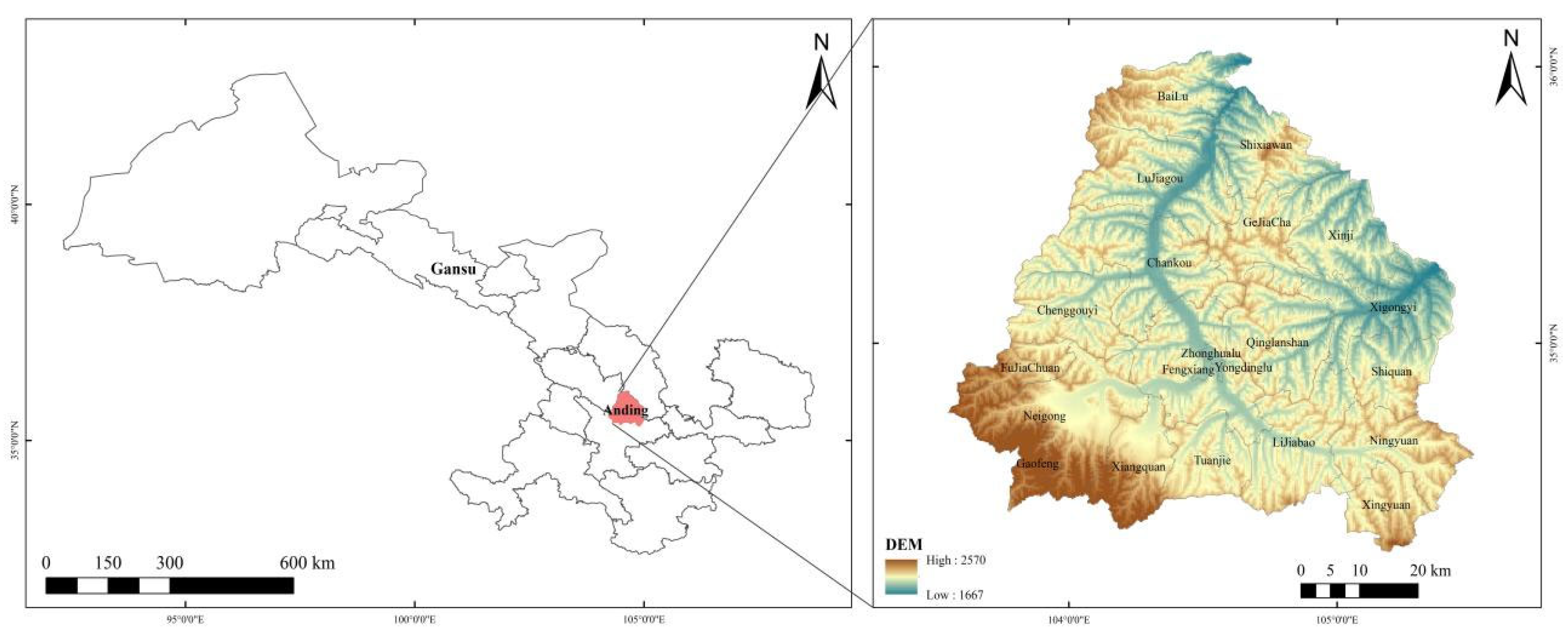
The study area was located in Dingxi Anjiapo Test Station, Gansu Province, which is a semi-arid agroclimate area in the middle of Gansu Province. It has a temperate continental climate, with an altitude of about 2000 m and an annual average temperature of about 6.4 °C. The average annual frost-free period is about 140 days and the average annual rainfall is 394 mm. The specific location of the test area is shown in Figure 1.
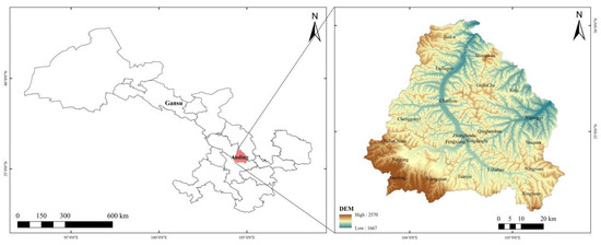
Figure 1.
The province in China where the research station is located.
Field experiments were conducted at Dingxi Anjiapo Test Station from 2020 to 2022. Dingxi No. 35 spring wheat was sown in mid-late March and harvested in August. Nitrogen in the form of urea at 110 kg · N · hm−2 (MN) was applied to each cell. In 2022, three fertilization gradients were added: ① no fertilizer (CK); ② low-concentration (LN) urea with nitrogen content of 55 kg·N·hm−2; and ③ high-concentration (HN) urea with nitrogen content of 220 kg·N·hm−2.
2.2. Data Source and N2O Gas Measurement Method
The meteorological data of the Anding District of Dingxi city from 1971 to 2022 were obtained from the Gansu Meteorological Bureau. Meteorological data contained daily temperature (°C), daily minimum temperature (°C), daily maximum temperature (°C), daily solar radiation (MJ·m−2), and daily precipitation (mm). In addition, the main soil property parameters of the study area were obtained as well. A crop variety module was created according to the experimental spring wheat variety used.
In order to determine the emission of N2O gas, static box-gas chromatography was used in the test area. Stainless steel bases were installed in the experimental area. A non-vented bottomless steel box was placed on the base. The static box was then wrapped with insulation sponge to ensure stable temperature during sample collection. Additionally, the top of the static box was equipped with two air stirring fans and the side of the box was equipped with a power plug for the fan, a gas sampling interface, and a temperature measurement interface. N2O gas collection was conducted every 20 days during the wheat growth season with a fixed sampling time from 9:00 a.m. to 11:00 a.m. (during which the atmospheric temperature was close to the daily average). A 100 mL sample was collected immediately following placement of the steel box (time = zero) using a syringe and sampling was repeated (100 mL) every 8 min for a total of 40 min. Simultaneously, the temperature inside the box was measured using a JM624 portable digital thermometer. Immediately after sampling, the sample was brought back to the laboratory for the concentration of N2O measurement using a gas chromatograph to determine the characteristics of N2O flux changes. The calculation of N2O emission flux refers to the calculation method of greenhouse gas emission intensity given by Timothy et al. [22].
2.3. Optimization Algorithm
The Drosophila Optimization Algorithm (Fruit Fly Optimization Algorithm, FOA) is a natural heuristic optimization algorithm [23]. It is a new swarm intelligence optimization algorithm based on the bionic principle of drosophila foraging behavior. The principle is easy to understand and easy to implement.
The algorithm simulates fly foraging behavior and food location through two mechanisms, olfactory and visual, thus enabling both global search and local search [24]. The basic process of the FOA includes five main steps: initialization of the population, olfactory search, visual search, fitness evaluation, and location update. First, the algorithm randomly generates the initial population, simulating the position of the Drosophila population. Next, the flies sense the location of food and move to a new location. The flies then complete local search visually, and the suitability of each position is determined by assessing its fitness score. The better the fitness value, the better the position. The algorithm then takes the position with the best fitness value as the current optimal position and updates the position of the Drosophila population from there. This process is repeated until the termination condition is met or the maximum number of iterations is reached.
The advantages of the traditional FOA algorithm lie in its simplicity and ease of realization, as well as its strong global search ability. However, due to the use of fixed steps, the traditional FOA algorithm has some limitations in dealing with complex optimization problems [25]. A fixed step size may cause the algorithm to ignore the complexity of the search space during the search. If the step size is too large, the global optimal solution may be bypassed; if the step size is too small, it may lead to a slow convergence rate, or even fall into a local optimum.
To overcome these limitations, the VSS-FOA algorithm introduces a dynamic step-size tuning mechanism [26]. It adjusts the step size according to the number of iterations or fitness values. A larger global search is used to cover the search space quickly, to reduce step size in later iterations, and to perform better local search in order to accurately find the global optimal solution. This method of dynamically adjusting the step size enables the VSS-FOA algorithm to balance global and local search better, and improve the adaptability and flexibility of the algorithm. Specifically, the VSS-FOA algorithm increases and reduces the step size even without improvement in the fitness function, ensuring that the algorithm can jump out of a local optimum and gradually approach the global optimum. Although the implementation complexity of VSS-FOA algorithm is slightly higher than the traditional FOA algorithm, it shows higher efficiency and accuracy in complex optimization problems, as well as stronger adaptability, and is able to search for the global optimal solution more effectively. Therefore, the VSS-FOA algorithm demonstrates significant advantages in practical applications, especially in complex optimization scenarios such as crop models.
The particular procedure of the FOA is outlined below:
- 1.
- Determine drosophila population size . Optimize the maximum number of iterations, , and the random initialization positions, and , of the drosophila population.
- 2.
- Set the random direction and distance of each Drosophila individual searching for food through smell. is the initial step parameter of an individual.
- 3.
- Since the specific location of the food remains unknown, the distance from the origin to each individual fruit fly must be calculated. Then, the determination of the value of the taste concentration can be obtained according to the value of this distance.
- 4.
- Si is then substituted into the fitness function to determine flavor concentration (Smelli).
- 5.
- The individual fruit fly with the highest taste concentration is then found.
- 6.
- The optimal value of the flavor concentration among the individual flies and the location coordinates are retained, and the flies are then assumed to fly to that location to perform visual search.
- 7.
- Redetermine the step parameter.
Here, is the initial step, stands for the current number of iterations, and stands for the maximum number of iterations. As the number of iterations increases, the value of the step parameter in the iteration process changes. In the initial iteration of the algorithm, the ability of this algorithm is most outstanding in global search because the step size parameter reaches its maximum value. However, with the increase in iteration times of the optimization algorithm with variable step size, the step size parameter gradually decreases, the local search ability of the algorithm gradually increases, and the search accuracy begins to improve. A dynamic balance between global optimization and local optimization is achieved.
- 8.
- Update the position of the individual flies.
- 9.
- Verify that the termination conditions are met. If reached, the iteration ends and the optimal solution is found. Otherwise, repeat (3)–(8) until the current number of iterations is equal to the maximum number of iterations or the fitness value reaches the predetermined threshold.
2.4. The APSIM Model
The APSIM model contains a series of modules designed to simulate biological and physical processes in agricultural systems that cover crop growth, soil moisture, carbon and nitrogen dynamics, changing climate, and the effects of management interventions and their interactions [27]. The APSIM model simulates the emission of N2O during nitrification and denitrification [21]. Nitrification and denitrification are considered to be the most important ways to release N2O from farmland soils [28,29]. Nitrification follows the reaction of crop dynamics to available ammonium in soil, and the nitrification rate (Rnit) is modeled as [30]:
The denitrification rate is combined with the ratio of N2 to N2O released during denitrification. N2O emissions can be predicted as follows [31,32].
The symbols and abbreviations in Equations (9)–(11) are explained in Table 1.

Table 1.
Formula symbols.
2.5. Parameter Optimization
2.5.1. The Fitness Function
In this study, the mean square error (Mean Squared Error, MSE), namely the mean square difference between the simulated value and measured value, was used as the fitness as follows:
In Formula (12), n represents the number of samples, yr represents the actual emission measurement of N2O, and ys is the simulated value of N2O output by the model.
2.5.2. Parameter Optimization Process
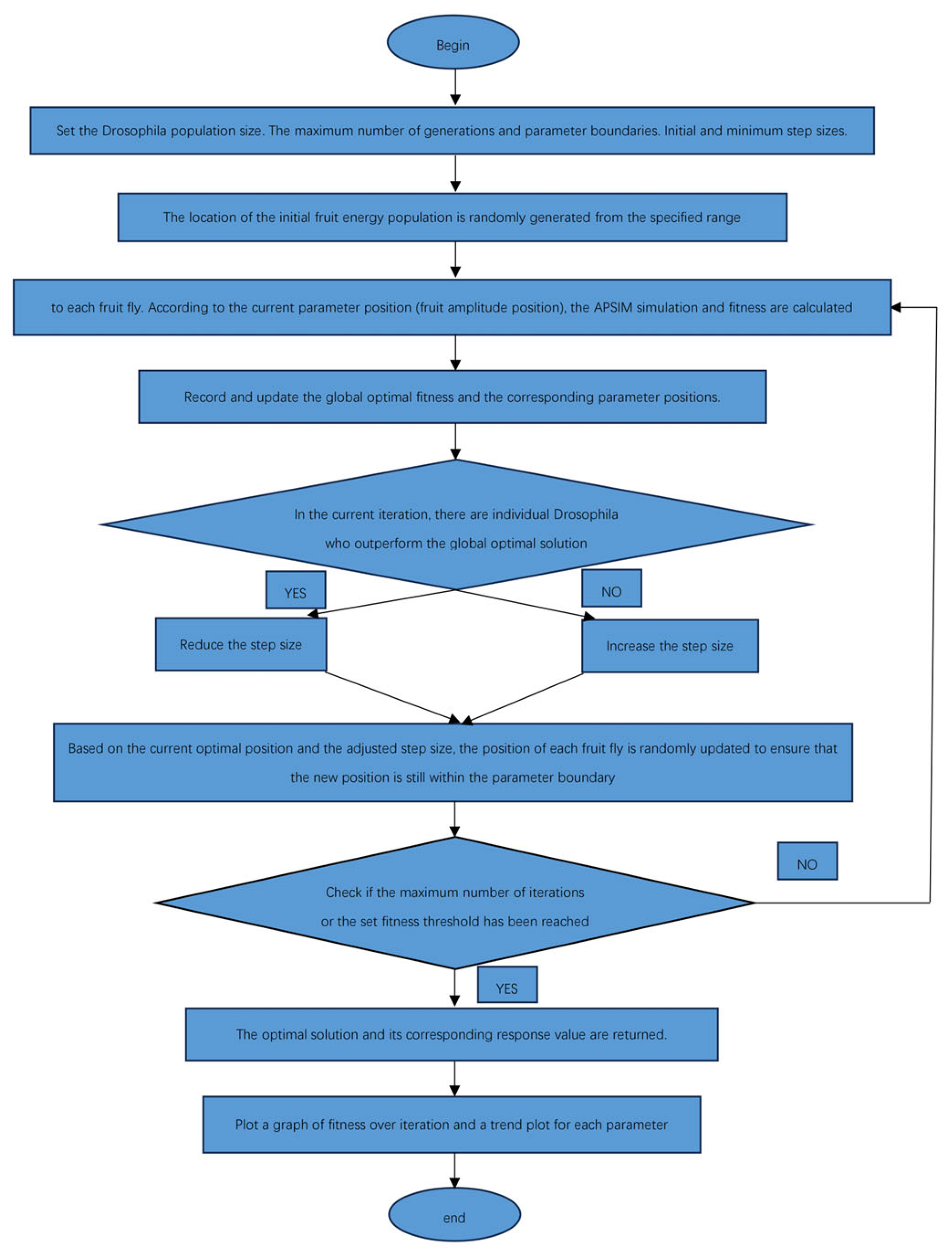
Figure 2 shows the flow chart for the VSS-FOA algorithm, which was adopted to optimize the parameters of N2O emission flux in the APSIM model. The specific steps are as follows:

Figure 2.
The variable step size FOA.
- Define the parameters and ranges.
Five parameters of soil N2O emission model in dry wheat fields were selected to optimize, along with minimum and maximum boundaries for each. The default values and ranges of the parameters in the model are shown in Table 2.

Table 2.
The parameter ranges that need to be adjusted.
- Initialize the algorithm.
The parameter position of the initial flight population is set to be randomly and evenly distributed in the above range, with a population size N of 20, a maximum number of iterations T of 200, an initial step size S0 of 10, and the final step size Sf of 0. We set the initialized no_improvement count (no_improvement_count) to 0, the no_improvement threshold (no_improvement_threshold) to 5, and the global optimal fitness value (best_smell_concentration_global) to infinity. The initial population position matrix was then randomly generated .
- Compute the fitness function.
For each parameter value, the expression in Formula (12) is used to compute the fitness function.
- Optimization.
First, at the beginning of each iteration, the step size is calculated based on the current number of iterations, and the step size is gradually reduced from initial_step_size to final_step_size. Then, for each individual fly in the population, its parameters are extracted and simulations are run to calculate the fitness, which is stored in an array (smell_concentration). In each current population, the individual fly with the smallest fitness value is found to be the best for each current iteration, meaning this fly has found the best parameter values.
The algorithm then determines whether the current best fitness value is better than the global optimal fitness value. If the current best fitness value is better than the global optimal fitness value, the global optimal fitness value is updated and the no_improvement counter no_improvement_count is reset to 0. Also, if the current step size is greater than the final step size, we multiply the step size by 0.9 to reduce it. If the current optimal fitness value does not improve the global optimal fitness value, the no_improvement counter (no_improvement_count) increments by 1. When no_improvement_count reaches the preset threshold no_improvement_threshold, the step size is multiplied by 1.1 to increase it.
During each iteration, the position of each fly in the population is updated for the adjusted step size while being restricted to remaining within the parameter boundaries. In this way, the algorithm gradually adjusts the step size and updates the fly position, while avoiding falling into a local optimal solution.
- Termination conditions.
If the maximum number of iterations is reached or the fitness value reaches a predetermined threshold, the algorithm is terminated, and the optimal position and corresponding fitness value are output.
- Data visualization.
Drawing fitness histories and paths taken toward optimality allow us to determine if any further step size adjustments are needed.
2.5.3. Model Calibration
The root mean square error (RMSE) and the standard root mean square error (NRMSE) were the two indicators used to measure the accuracy of the model by evaluating the agreement between the simulated values from the model and the measured values. The RMSE denotes the mean discrepancy between the simulated outcomes and the empirical data [33], and is frequently used as an important indicator of model error. A smaller RMSE value indicates higher accuracy [34]. NRMSE is a standard statistic used to calculate the error between simulated and measured values by comparing their relative differences.
The formulas used for model testing are in Formulas (13) and (14):
where is the number of observed points, is the maximum of the observed value, and is the minimum of the observed value. In Formula (13), the variables are the observed values, and the variables are the simulated values.
2.5.4. Scenario Design for Nitrogen Application Rates
The APSIM model with optimized parameters was used to simulate the N2O emission flux response values under different nitrogen fertilizer rates in 2022. The FerOnEvent (event fertilization) component was added to the Manager folder module in the APSIM model, setting the fertilization event as wheat sowing and nitrogen fertilizer rate at 0 kg·N·hm−2, 55 kg·N·hm−2, 220 kg·N·hm−2, simulated N2O emissions flux.
3. Results
3.1. Optimization Results
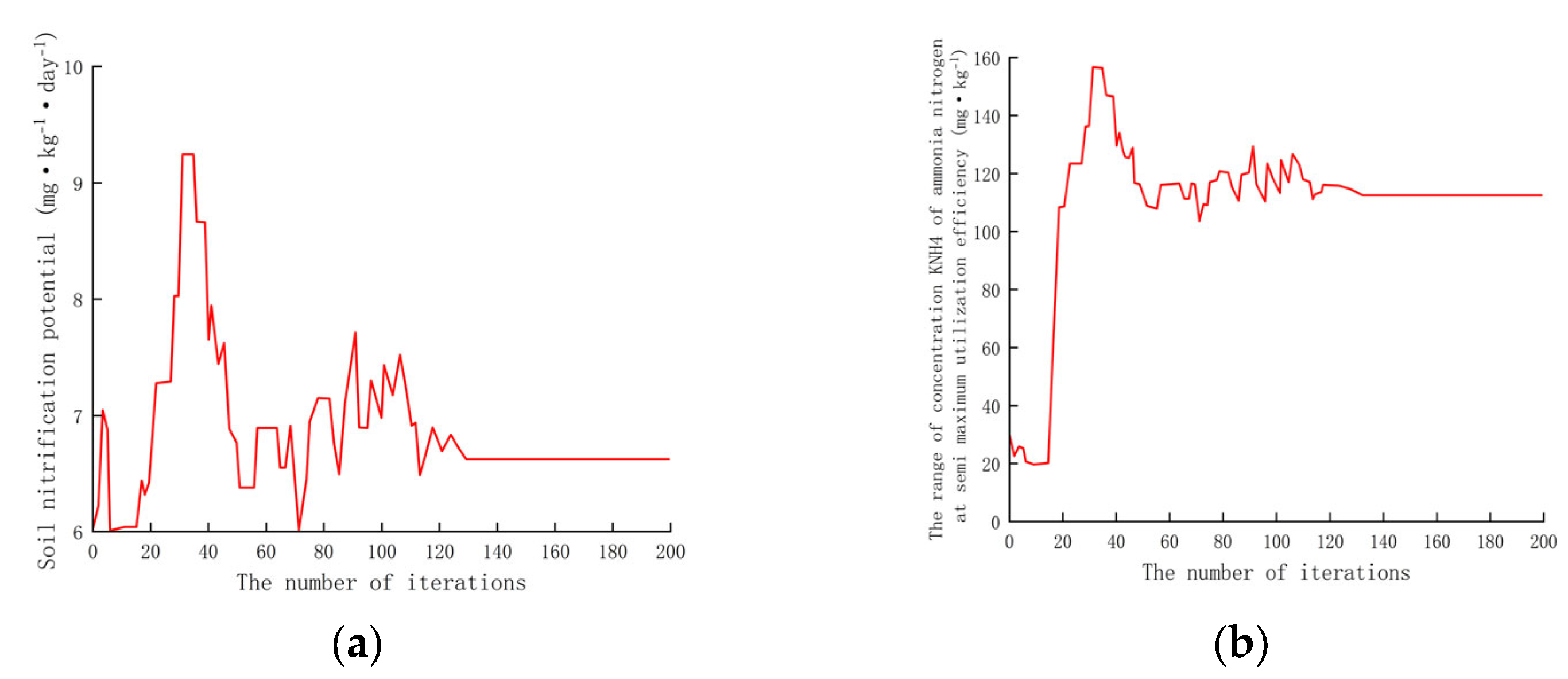
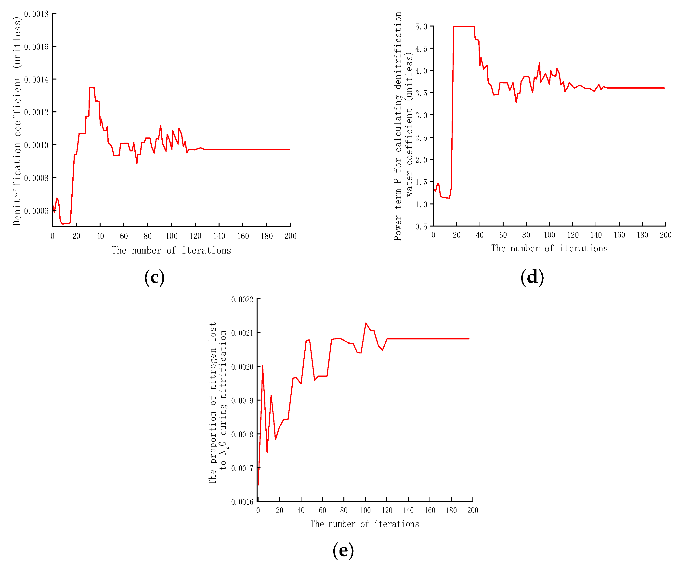
During the course of the optimization run, we observed that when the global search number T reached about 125, the algorithm started to converge and the fitness value stabilized, meaning that a further search did not significantly affect the results.
Given the meta-heuristic randomness of the algorithm, each run may produce different optimization results as well. Therefore, multiple runs of the program are required in order to obtain more reliable and stable optimization results. We, therefore, ran the algorithm five times to reduce the influence of random factors on the final outcome. After each program run, the optimization results were recorded and analyzed, and the average of the five runs was taken as the final optimization result.
The default values of the five parameters to be optimized are shown in Table 3. To analyze the effect of the optimization on the chosen parameters, we created a plot (Figure 3). From the plot we can see that nitrification_pot, nh 4_at_half_pot, nit_N2O_frac, dnit_rate_coeff, and dnit_wf_power fluctuated greatly at the beginning of the iteration, but gradually stabilized as the number of iterations increased. The trend in the fitness values during the optimization process is very consistent. With an increasing number of iterations, the fitness value is reduced from 4 to 0.3.

Table 3.
Comparison between default and optimized values of model parameters to be optimized.
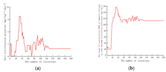
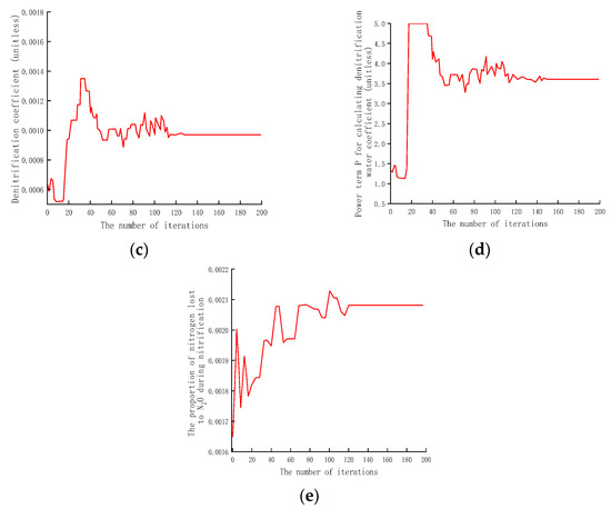
Figure 3.
The changes in 5 parameter values during the iterative optimization process. (a) The change in soil nitrification potential; (b) the change in the range of concentrations in KNH4 of ammonia and nitrogen at semi-maximum utilization efficiency; (c) the change in denitrification coefficient; (d) the change in the power term P for calculating denitrification water coefficient; and (e) the change in the proportion of nitrogen loss to N2O during the nitrification process.
3.2. Model Calibration Results
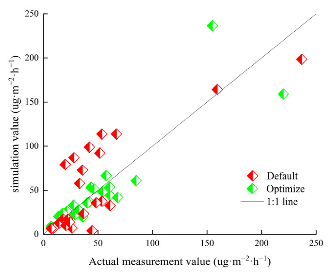
After the optimization using the VSS-FOA algorithm, wheat field soil N2O emissions’ flux were simulated to ascertain the accuracy of the model. The model performance was significantly improved after parameter optimization with the VSS-FOA algorithm compared to using the APSIM default parameters, as shown in Table 4. The optimized R2 increased from 0.413 to 0.739, and the NRMSE decreased from 17.1% to 11.4%.

Table 4.
Comparison of results before and after parameter optimization.
The effects of using the default values, optimized values, and measured values of soil N2O emissions flux in the sample wheat field are shown in Figure 4. The results show that after parameter optimization, the fitting curve of the simulated values and measured values is closer to the 45-degree line than with using the defaults alone, indicating the enhanced consistency of the model predictions with the observed values. Parameter optimization significantly improved the reliability and accuracy of the model with respect to the actual emission simulation.

Figure 4.
Comparison of default, measured, and optimized N2O emission flux from 2020–2022.
3.3. Simulation of N2O Emission Flux at Different Nitrogen Application Rates
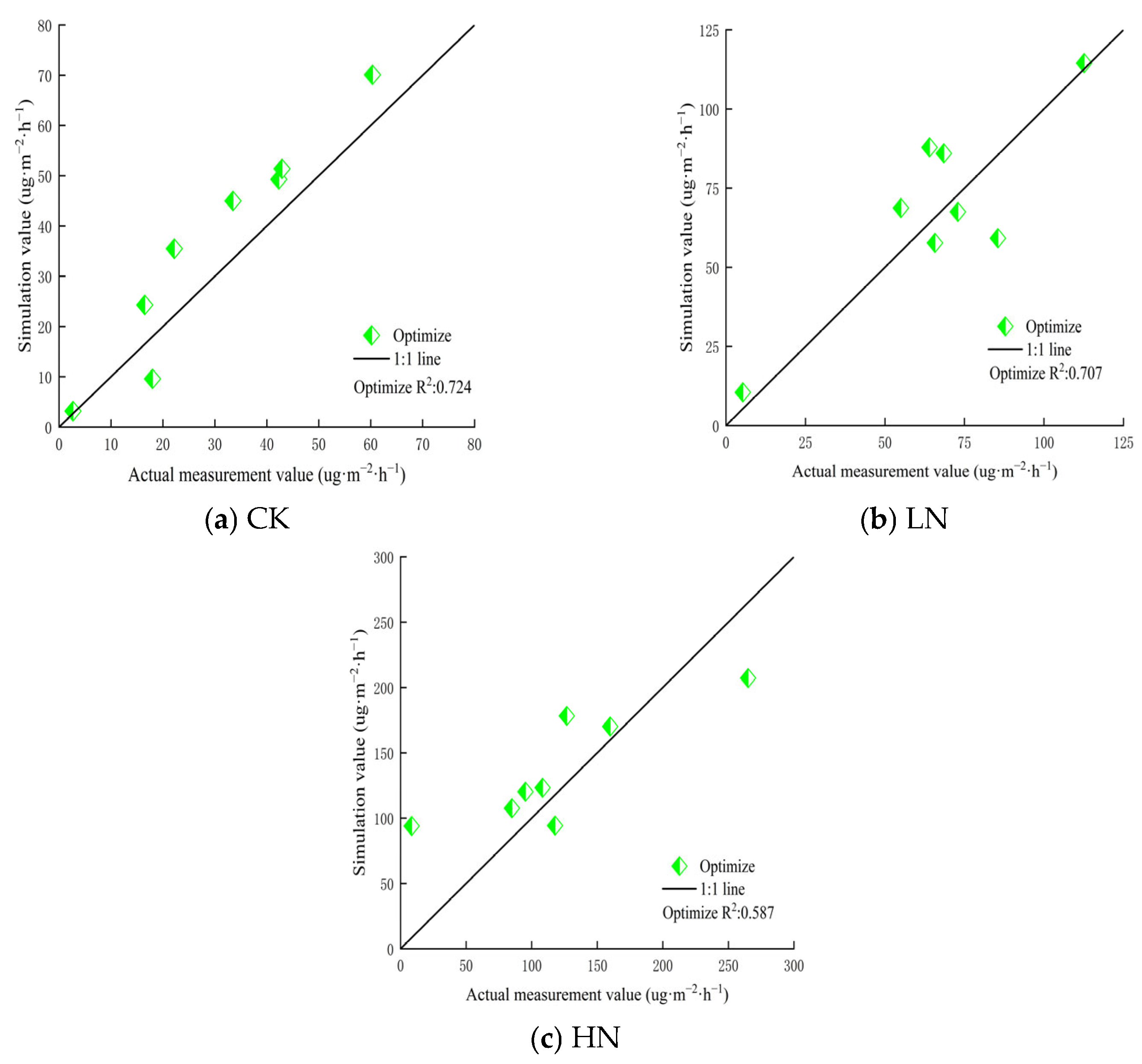
The fits of the simulated and measured values under CK, LN, and HN are shown in Figure 5. After the five parameters of the APSIM model were optimized using the VSS-FOA algorithm, however, the degree of fit between the two was significantly improved under the three different nitrogen rates. Specifically, the simulated value of the model of N2O emissions’ flux has the best agreement under CK treatment, with an R2 value of 0.724. Under HN treatment, the simulated value of the model is also somewhat consistent with the measured value, with an R2 value of 0.587.
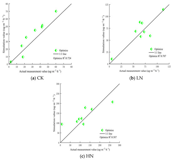
Figure 5.
The simulation results of N2O emissions’ flux under different nitrogen application rates in 2022.
4. Discussion
4.1. Model Optimization Effects
N2O emission flux in fields are influenced by multiple factors such as the soil pH and nitrogen fertilization [35], and the APSIM model has been widely validated and applied globally to provide reliable predictions for it in different climates and soil conditions [36]. This broad applicability, coupled with its high parametric ability to model complex crop ecosystems, makes it an ideal tool for studying and simulating N2O emission flux and their management strategies. In this study, five parameters related to N2O emission flux were optimized by the VSS-FOA algorithm, which improved the applicability and parameter rate efficiency of the model in dry farmland compared to default parameter values. The process of parameter optimization fully considers crop growth patterns and multiple environmental factors and can improve the accuracy of N2O emission flux prediction in the APSIM model while not affecting predictions about other important biochemical processes during crop growth and development. Compared to the default parameter values of the APSIM model, the R² increased from 0.413 to 0.739 and the NRMSE decreased from 17.1% to 11.4%, indicating that the model optimized by the VSS-FOA algorithm showed had accuracy and consistency with the measured value of N2O emission flux in the study area.
Rafique et al. proposed an algorithm calibration method for global optimal parameters of constrained models. Applying this algorithm to DayCent model calibration, the residual difference between the simulated and observed values in N2O emission flux was greatly reduced, and the coefficient of determination between the observed and simulated values of N2O emission flux was significantly improved [37]. In this study, however, the VSS-FOA algorithm was more flexible and efficient. We effectively enhanced the global search capability as well as the local search accuracy by introducing a dynamic step size adjustment mechanism. In the early stage of optimization, the algorithm uses larger steps for the global search to quickly cover the search space, but gradually reduces the step size in the later iteration to avoid falling into a local optimum. This approach not only simplifies the optimization process, but also improves the efficiency and accuracy of dealing with complex optimization problems and is especially suitable for complex scenarios that require global optimization and a localized fine search.
Tang et al. found that among many crop models, the APSIM model was more effective in simulating wheat field N2O emission flux [38], and Li et al. optimized the APSIM model by adjusting the ratio of nitrate nitrogen converted to N2O-N (K2 value) and optimizing only one parameter in the model [39]. In contrast, the VSS-FOA algorithm used in this study jointly optimized all five parameters in the model, improving the model’s direct applicability to the study area.
In terms of the overall optimization of the model, even the R2 and model prediction indicators showed improvement after calibration and optimization. The fit of the model is high at low values (<100 µg·hm−2·h−1), but individual higher values are not well simulated. This is because the algorithm considers the overall performance of the model and cannot change other parameter requirements because of one or two extreme data points; only the minimum fitness function is calculated in the optimization result.
4.2. Study Limitations and Perspectives
This study has presented some novel results in N2O emission simulation and optimization, but it still has some limitations. Three years of soil N2O emission data from the study area were used for optimization and validation, and because climate, soil properties, and field management practices can vary significantly from year to year, such short-time-span data may not adequately capture these changes. Therefore, in order to improve the stability and universal applicability of the model, future studies need to increase the intensity of the sampling effort.
5. Conclusions
In this study, a VSS-FOA algorithm was used to optimize N2O emission flux parameters in the APSIM model, and the effects of different nitrogen rates on soil N2O emission flux were simulated. The applicability of the APSIM model is improved through the calibration of model parameters, which lays a foundation for the localized application of the model.
The parameters of soil N2O emission flux optimization in the dry wheat field studied were a soil nitrification potential of 6.63, a range of concentration of ammonia and nitrogen at semi-maximum utilization efficiency of 112.4, proportion of nitrogen loss to N2O during nitrification of 0.002, denitrification coefficient of 0.0009, and power term P for calculating denitrification water coefficient of 3.58. The R2 of the simulated and measured values in the model under CK, LN, and HN treatment levels were 0.724, 0.707, and 0.587, respectively.
Author Contributions
Conceptualization, L.D. and S.M.; methodology, L.D.; software, S.M.; validation, L.D., G.L., and S.M.; formal analysis, L.D.; investigation, L.D.; resources, G.L.; data curation, L.D.; writing—original draft preparation, L.D.; writing—review and editing, L.D., G.L., and S.M.; visualization, S.M.; supervision, G.L.; project administration, G.L. and L.D.; funding acquisition, G.L. All authors have read and agreed to the published version of the manuscript.
All authors have read and agreed to the published version of the manuscript.
Funding
This research was financed by the Nature Science Foundation of China through the research grant 32360438.
Data Availability Statement
Data are contained within the article.
Conflicts of Interest
The authors declare no conflicts of interest.
References
- Oulaid, B.; Milne, A.E.; Waine, T.; El Alami, R.; Rafiqi, M.; Corstanje, R. Stepwise model parametrisation using satellite imagery and hemispherical photography: Tuning AquaCrop sensitive parameters for improved winter wheat yield predictions in semi-arid regions. Field Crop. Res. 2024, 309, 109327. [Google Scholar] [CrossRef]
- Soltani, A.; Alimagham, S.M.; Nehbandani, A.; Torabi, B.; Zeinali, E.; Dadrasi, A.; Zand, E.; Ghassemi, S.; Pourshirazi, S.; Alasti, O.; et al. SSM-iCrop2: A simple model for diverse crop species over large areas. Agric. Syst. 2020, 182, 102855. [Google Scholar] [CrossRef]
- Gunarathna, M.H.J.P.; Sakai, K.; Kumari, M.K.N. Emulator-based optimization of APSIM-Sugar using the results of sensitivity analysis performed with the software GEM-SA. Front. Sustain. Food Syst. 2023, 7, 1157854. [Google Scholar] [CrossRef]
- Lisson, S.N.; Inman-Bamber, N.G.; Robertson, M.J.; Keating, B.A. The historical and future contribution of crop physiology and modelling research to sugarcane production systems. Field Crop. Res. 2005, 92, 321–335. [Google Scholar] [CrossRef]
- Ngwira, A.R.; Aune, J.B.; Thierfelder, C. DSSAT modelling of conservation agriculture maize response to climate change in Malawi. Soil Tillage Res. 2014, 143, 85–94. [Google Scholar] [CrossRef]
- Tsakmakis, I.D.; Zoidou, M.; Gikas, G.D.; Sylaios, G.K. Impact of irrigation technologies and strategies on cotton water footprint using AquaCrop and CROPWAT models. Environ. Process. 2018, 5, 181–199. [Google Scholar] [CrossRef]
- Zhang, Y.; Walker, J.P.; Pauwels, V.R. Assimilation of wheat and soil states for improved yield prediction: The APSIM-EnKF framework. Agric. Syst. 2022, 201, 103456. [Google Scholar] [CrossRef]
- Heslot, N.; Akdemir, D.; Sorrells, M.E.; Jannink, J.L. Integrating environmental covariates and crop modeling into the genomic selection framework to predict genotype by environment interactions. Theor. Appl. Genet. 2014, 127, 463–480. [Google Scholar] [CrossRef]
- Schauberger, B.; Archontoulis, S.; Arneth, A.; Balkovic, J.; Ciais, P.; Deryng, D.; Elliott, J.; Folberth, C.; Khabarov, N.; Müller, C.; et al. Consistent negative response of US crops to high temperatures in observations and crop models. Nat. Commun. 2017, 8, 13931. [Google Scholar] [CrossRef]
- Akhavizadegan, F.; Ansarifar, J.; Wang, L.; Huber, I.; Archontoulis, S.V. A time-dependent parameter estimation framework for crop modeling. Sci. Rep. 2021, 11, 11437. [Google Scholar] [CrossRef]
- Keating, B.A.; Robertson, M.J.; Muchow, R.C.; Huth, N.I. Modelling sugarcane production systems I. Development and performance of the sugarcane module. Field Crop. Res. 1999, 61, 253–271. [Google Scholar] [CrossRef]
- Sexton, J.; Everingham, Y.L.; Inman-Bamber, G. A global sensitivity analysis of cultivar trait parameters in a sugarcane growth model for contrasting production environments in Queensland, Australia. Eur. J. Agron. 2017, 88, 96–105. [Google Scholar] [CrossRef]
- Preecha, K.; Sakai, K.; Pisanjaroen, K.; Sansayawichai, T.; Cho, T.; Nakamura, S.; Nakandakari, T. Calibration and Validation of Two Crop Models for Estimating Sugarcane Yield in Northeast Thailand. Trop. Agric. Dev. 2016, 60, 31–39. [Google Scholar]
- Mthandi, J.; Kahimba, F.C.; Tarimo, A.K.; Salim, B.A.; Lowole, M.W. Modification, Calibration and Validation of APSIM to Suit Maize (Zea mays L.) Production System: A Case of Nkango Irrigation Scheme in Malawi. Am. J. Agric. For. 2014, 13, 1–11. [Google Scholar]
- Sun, H.; Zhang, X.; Wang, E.; Chen, S.; Shao, L.; Qin, W. Assessing the Contribution of Weather and Management to the Annual Yield Variation of Summer Maize Using APSIM in the North China Plain. Field Crop. Res. 2016, 194, 94–102. [Google Scholar] [CrossRef]
- Seidel, S.J.; Palosuo, T.; Thorburn, P.; Wallach, D. Towards Improved Calibration of Crop Models—Where Are We Now and Where Should We Go? Eur. J. Agron. 2018, 94, 25–35. [Google Scholar] [CrossRef]
- Harrison, M.T.; Roggero, P.P.; Zavattaro, L. Simple, Efficient and Robust Techniques for Automatic Multi-Objective Function Parameterisation: Case Studies of Local and Global Optimisation Using APSIM. Environ. Model. Softw. 2019, 117, 109–133. [Google Scholar] [CrossRef]
- Cui, W.; Nie, Z.; Li, G.; Yuan, J. Optimization of Parameters Related to Grain Growth of Spring Wheat in Dryland Based on the Next-Generation APSIM. Agronomy 2023, 13, 1915. [Google Scholar] [CrossRef]
- Guo, D.; Olesen, J.E.; Pullens, J.W.; Guo, C.; Ma, X. Calibrating AquaCrop model using genetic algorithm with multi-objective functions applying different weight factors. Agron. J. 2021, 113, 1420–1438. [Google Scholar] [CrossRef]
- Bandara, W.B.M.A.C.; Sakai, K.; Nakandakari, T.; Kapetch, P.; Anan, M.; Nakamura, S.; Setouchi, H.; Rathnappriya, R.H.K. Global Optimization of Cultivar Trait Parameters in the Simulation of Sugarcane Phenology Using Gaussian Process Emulation. Agronomy 2021, 11, 1379. [Google Scholar] [CrossRef]
- Wang, W.G.; Luo, L.Z.; Wang, W.E.; Zhang, Z.W. Reducing greenhouse gas emissions while maintaining yield in the croplands of Huang-Huai-Hai Plain, China. Agr. For. Meteorol. 2018, 260, 80–94. [Google Scholar] [CrossRef]
- Timothy, H.; Jonathan, P.; Kevin, B. Target—Intensity: Ananalysis of Greenhouse Gas Intensity Targets; World Resources Institute: Washington, DC, USA, 2006; p. 37. [Google Scholar]
- Pan, W.T. A new fruit fly optimization algorithm: Taking the financial distress model as an example. Knowl.-Based Syst. 2012, 26, 69–74. [Google Scholar] [CrossRef]
- Ranjan, R.K.; Kumar, V. A systematic review on fruit fly optimization algorithm and its applications. Artif. Intell. Rev. 2023, 56, 13015–13069. [Google Scholar] [CrossRef]
- Qisong, Q.; Gening, X.; Xiaoning, F.; Jun, W. A new type bionic global optimization: Construction and application of modified fruit fly optimization algorithm. Proc. Inst. Mech. Eng. Part B-J. Eng. Manuf. 2015, 229, 1614–1621. [Google Scholar] [CrossRef]
- Huang, H.; Tao, D.; Wei, X.; Zhou, Y. Adaptive Image Enhancement Algorithm Based on Variable Step Fruit Fly Optimization Algorithm and Nonlinear Beta Transform. Biomimetics 2023, 8, 212. [Google Scholar] [CrossRef] [PubMed]
- Keating, B.A. APSIM’s origins and the forces shaping its first 30 years of evolution: A review and reflections. Agron. Sustain. Dev. 2024, 44, 24. [Google Scholar] [CrossRef]
- Baggs, E.M.; Smales, C.L.; Bateman, E.J. Changing pH shifts the microbial source as well as the magnitude of N2O emission from soil. Biol. Fert. Soils. 2010, 46, 793–805. [Google Scholar] [CrossRef]
- Wrage, N.; Groenigen, J.W.; Oenema, O.; Baggs, E.M. A novel dual-isotope labelling method for distinguishing between soil sources of N2O. Rapid Commun. Mass Spectrom. 2005, 19, 3298–3306. [Google Scholar] [CrossRef]
- Parton, W.J.; Holland, E.A.; Del Grosso, S.J.; Hartman, M.D.; Martin, R.E.; Mosier, A.R.; Schimel, D.S. Generalized model for NOx and N2O emissions from soils. J. Geophys. Res. Atmos. 2001, 106, 17403–17419. [Google Scholar] [CrossRef]
- Del Grosso, S.J.; Ojima, D.S.; Parton, W.J.; Stehfest, E.; Heistemann, M.; DeAngelo, B.; Rose, S. Global scale DAYCENT model analysis of greenhouse gas emissions and mitigation strategies for cropped soils. Glob. Planet. Chang. 2009, 67, 44–50. [Google Scholar] [CrossRef]
- Thorburn, P.J.; Biggs, J.S.; Collins, K.; Probert, M.E. Using the APSIM model to estimate nitrous oxide emissions from diverse Australian sugarcane production systems. Agric. Ecosyst. Environ. 2010, 136, 343–350. [Google Scholar] [CrossRef]
- Guo, Q.; Wu, W. Application of parameter optimization methods based on Kalman formula to the soil—Crop system model. Int. J. Environ. Res. Public Health 2023, 20, 4567. [Google Scholar] [CrossRef] [PubMed]
- Wang, Y.; Huang, D.; Sun, K.; Shen, H.; Xing, X.; Liu, X.; Ma, X. Multiobjective optimization of regional irrigation and nitrogen schedules by using the CERES-Maize model with crop parameters determined from the remotely sensed leaf area index. Agric. Water Manag. 2023, 286, 108386. [Google Scholar] [CrossRef]
- Wu, G.; Liang, F.; Wu, Q.; Feng, X.G.; Shang, W.D.; Li, H.W.; Song, H. Soil pH differently affects N2O emissions from soils amended with chemical fertilizer and manure by modifying nitrification and denitrification in wheat-maize rotation system. Biol. Fert. Soils. 2024, 60, 101–113. [Google Scholar] [CrossRef]
- Cao, H.; Gao, D.; Zhang, W.; Zhang, W.; Chen, J.; Li, W.; Wang, F. Developmental analysis and application examples for agricultural models. Smart Agric. 2020, 2, 147. [Google Scholar]
- Rafique, R.; Kumar, S.; Luo, Y.; Kiely, G.; Asrar, G. An algorithmic calibration approach to identify globally optimal parameters for constraining the DayCent model. Ecol. Modell. 2015, 297, 196–200. [Google Scholar] [CrossRef]
- Tang, Y.; Qiao, Y.; Ma, Y.; Huang, W.; Komal, K.; Miao, S. Quantifying Greenhouse Gas Emissions in Agricultural Systems: A Comparative Analysis of Process Models. Ecol. Model. 2024, 490, 110646. [Google Scholar] [CrossRef]
- Li, T.T.; Zhang, W.; Wang, J.; Zhang, W.; Wang, G.C.; Xu, J.J.; Zhang, Q. Parameterizing an Agricultural Production Model for Simulating Nitrous Oxide Emissions in a Wheat–Maize System in the North China Plain. Atmos. Oceanic Sci. Lett. 2016, 9, 403–410. [Google Scholar] [CrossRef]
Disclaimer/Publisher’s Note: The statements, opinions and data contained in all publications are solely those of the individual author(s) and contributor(s) and not of MDPI and/or the editor(s). MDPI and/or the editor(s) disclaim responsibility for any injury to people or property resulting from any ideas, methods, instructions or products referred to in the content. |
© 2024 by the authors. Licensee MDPI, Basel, Switzerland. This article is an open access article distributed under the terms and conditions of the Creative Commons Attribution (CC BY) license (https://creativecommons.org/licenses/by/4.0/).

