Estimation of Surface Ozone Effects on Winter Wheat Yield across the North China Plain

Abstract

Surface ozone (O₃) pollution has adverse impacts on the yield of winter wheat. The North China Plain (NCP), one of the globally significant primary regions for winter wheat production, has been frequently plagued by severe O₃ pollution in recent years. In this study, the effects of O₃ pollution on winter wheat yield and economic impact were evaluated in the NCP during the 2015–2018 seasons using the regional atmospheric chemical transport model (WRF-Chem), O₃ metrics including the phytotoxic surface O₃ dose above 12 nmol m⁻² s⁻¹ (POD₁₂), and the accumulated daytime O₃ above 40 ppb (AOT40). Results showed that the modeled O₃, exposure-based AOT40, and flux-based POD₁₂ increased during the winter wheat growing season from 2015 to 2018. The annual average daytime O₃, exposure-based AOT40, and flux-based POD₁₂ were 44 ppb, 5.32 ppm h, and 1.78 mmol m⁻², respectively. During 2015–2018, winter wheat relative production loss averaged 10.9% with AOT40 and 14.6% with POD₁₂. This resulted in an average annual production loss of 12.4 million metric tons, valued at approximately USD 4.5 billion. This study enhances our understanding of the spatial sensitivity of winter wheat to O₃ impacts, and suggests that controlling O₃ pollution during the key growth stages of winter wheat or improving its O₃ tolerance will enhance food security.

1. Introduction

Surface ozone (O₃) is produced by precursors including VOCs (volatile organic compounds) and NOx (nitrogen oxides) by photochemical reactions [1]. It has strong oxidative potential. In recent years, the surface O₃ pollution in China exceeded that in other developed regions in the northern hemisphere, including Europe and the USA [2]. Some studies have shown that the developed regions of China have the most severe O₃ pollution; these regions include the Yangtze River Delta (YRD), the North China Plain (NCP), and the Pearl River Delta (PRD) [3,4,5,6,7]. High concentrations of ground-level O₃ have significant adverse impacts on climate, human health, and ecosystems [8,9,10,11]. Studies have established the exposure- and flux-based O₃ response relationships of crop yield using the Free Air-Controlled Exposure (FACE), and the Open Top Chambers (OTC) in Asia and Europe [12,13,14,15,16].

The accumulated daytime surface O₃ above 40 ppb (AOT40) was the most commonly used O₃ exposure metric, because it is easy to calculate, is significantly associated with the relative crop production [9,17,18,19], and is well established in both Europe and Asia [12,20,21]. Previous studies have used the AOT40 to evaluate the production reduction of crop attribute to surface O₃ pollution [4,7,9,18]. Unfortunately, the AOT40 is calculated only using the O₃ concentrations at canopy height, which leads to uncertainty to estimate impacts on crops [15,22].

The phytotoxic dose of ground-level O₃ above y nmol m⁻² s⁻¹ (POD_y) is used to evaluate hydrothermal conditions of crop growth areas [5,9,12,15,22]. Previous studies showed that POD_y is likely to be more accurate than O₃ exposure-based metrics (e.g., AOT40) [9,12,23] because it is calculated using O₃ concentrations at a 1 m height and stomatal uptake [12,14]. Therefore, the POD_y have been established for specific crops, including wheat [13,15], soybean [14,24], maize [12,22], potato [16], and rice [24,25].

The NCP is one of the main winter wheat-producing areas in China, accounting for 57% of the total yield in the country. Some studies have shown that the NCP also has some of the most serious O₃ pollution [4,5,22,26] due to its industry and agriculture, both of which provide abundant O₃ precursors (NOx, VOCs, etc.). Studies based on observational data showed that high O₃ pollution has reduced crop production in the NCP [5,26]. These studies assessed crop production using a single O₃ concentration index, AOT40, without considering other possibly relevant conditions such as water and heat during the growing season of the crop [5,15,27]. Moreover, O₃ levels were determined mainly at sparse monitoring stations in urban areas, leading to some uncertainty in the accuracy of the results.

In this study, hourly meteorological data and surface O₃ concentrations in the growing seasons of winter wheat during 2015–2018 in the NCP were simulated using the Weather Research and Forecasting model coupled with Chemistry (WRF-Chem). The main objectives were to determine spatio-temporal differences between the surface O₃, AOT40, and POD₁₂ (phytotoxic dose of ground-level O₃ above 12 nmol m⁻² s⁻¹), and to calculate yield losses and economic reduction caused by surface O₃ pollution during this period.

2. Materials and Methods

2.1. Data Sources

Hourly surface O₃ concentration data across the NCP from 2015 to 2018, including 850 stations for model validation, were obtained from the China National Environmental Monitoring Center (http://www.cnemc.cn/) (accessed on 7 October 2024). These data were measured using ultraviolet fluorescence methods, calibrated, and rigorously quality-controlled according to the National Ambient Air Quality Standards. The winter wheat production (WP) data, encompassing 321 counties across the NCP (shown in Figure S1), formed the basis for estimating the losses in WP caused by O₃. These WP data were obtained from the China Statistical Yearbook and compiled from surveys conducted by the official county-level statistical bureaus (http://www.stats.gov.cn/) (accessed on 7 October 2024). The timing data of winter wheat phenology periods, obtained from the agricultural meteorological monitoring stations (110 stations across the NCP) operated by the China Meteorological Administration, served as a crucial basis for defining the flowering period of winter wheat in this study.

2.2. Configurations of WRF-Chem Model

Hourly meteorological data and surface O₃ during the growing seasons (February–June) of winter wheat were simulated by the regional atmospheric chemical transport model (WRF-Chem v3.8.1). The meteorological and chemical processes in the atmosphere were simultaneously simulated by the online atmospheric chemical transport model (WRF-Chem) [28]. The two domains in WRF-Chem were adopted in the simulations of this study (Figure 1). Domain 1 (D01) and Domain 2 (D02) are simulation boundaries, which were projected on Lambert conformal grids (D01: 185 × 128 grid cells; D02: 166 × 184 grid cells) with horizontal resolutions of 27 km (D01) and 9 km (D02). In the simulation, the vertical dimension during the 100 hPa surface was 28 layers in WRF-Chem.

The detailed chemistry and physics configurations in WRF-Chem were the same as those by Wang et al. [9]. CBM-Z [29] and Madronich F-TUV [30] were the gas-phase chemistry mechanism and the photolysis scheme in WRF-Chem, respectively. The aerosol scheme used the MOSAIC-4A (Model for Simulating Aerosol Interaction and Chemistry with 4-sectional aerosol bins, including aqueous reactions) [31]. Performance of the simulated O₃ concentrations was evaluated using the Mean Bias (MB), Root Mean Square Error (RMSE), Correlation Coefficient (R), and the significance levels for the Correlation Coefficients (p-value) of the O₃ measurements at the 850 stations in D02. For detailed calculation methods, see Wang et al. [9].

The boundary conditions of chemistry were initialized using the Community Atmosphere Model coupled to Chemistry (CAM-Chem) [32]. The meteorological boundary conditions were initialized using the FNL datasets (National Center for Environmental Prediction Final Analysis) with 26 pressure levels, a horizontal resolution of 1° × 1°, and temporal resolution of 6 h. The MEIC v1.3 (Multi-resolution Emission Inventory for China with a resolution of 0.25° × 0.25° was used as anthropogenic emissions [33]. The simulation in 2015 adopted the MEIC of 2014, while the simulations from 2016 to 2018 used the MEIC of 2016. The Fire Inventory from NCAR data (FINN v1.5) with a horizontal resolution of 1 km × 1 km was adopted to calculate the biomass burning emissions [34]. The Model of Emissions of Gases and Aerosols from Nature (MEGAN) was adopted to provide the biogenic emission [35].

2.3. Calculation of POD₁₂ and AOT40

The AOT40 was calculated at the county scale using the hourly surface O₃ provided by WRF-Chem from 30 days after to 44 days before mid-flowering of the wheat [20]. Because there is a vertical gradient of O₃ concentrations, we converted the simulated O₃ of 25 m in height to 1 m in height using the method of Pleijel [36]. The specific formula below was used to calculate the AOT40:

$$\mathrm{AOT}40\left(\mathrm{ppb}\mathrm{h}\right)={\sum }_{\mathrm{i}=1}^{\mathrm{n}}({\left[{\mathrm{O}}_3\right]}_{\mathrm{i}}-40),{\left[{\mathrm{O}}_3\right]}_{\mathrm{i}}>40\mathrm{ppb}$$

(1)

where “[O₃]_i” is the daytime O₃ concentration at 1 m above the ground during 08:00–18:00. n is all hours in the winter wheat’s growing season.

The stomatal conductance (g_sto) was calculated by the Jarvis multiplicative model using data from February to June for the meteorological and environmental variables [37,38]. Based on a field study in Jiangsu, the equation for calculating g_sto was developed by Feng et al. [15], and is as follows:

$${\mathrm{g}}_{\mathrm{sto}}={\mathrm{g}}_{\max }\times \min \left({\mathrm{f}}_{\mathrm{phen}},{\mathrm{f}}_{{\mathrm{O}}_3}\right)\times {\mathrm{f}}_{\mathrm{light}}\times \max \left[{\mathrm{f}}_{\min },{\mathrm{f}}_{\mathrm{VPD}}\right]$$

(2)

where g_sto is actual stomatal conductance of surface O₃ (mmol O₃ m⁻² s⁻¹). f_min is minimum daytime g_sto. g_max is the maximum stomatal conductance (mmol O₃ m⁻² s⁻¹). The f_VPD, f_O3, f_phen, and flight represent the influence of the VPD (vapor pressure deficit), O₃ at 1 m, phenology, and photosynthetically active radiation, respectively. The detailed g_sto in Table S1 is an updated and localized parameter based on a field study in China. The stomatal conductance was calculated by Formulas (S1)–(S8) in the Supplementary Materials.

The flux-ozone of winter wheat leaves (F_st, in nmol m⁻² s⁻¹) was calculated based on the below specific equation:

$${\mathrm{F}}_{\mathrm{st}}=\left[{\mathrm{O}}_3\right]\times {\displaystyle \frac{1}{{\mathrm{r}}_{\mathrm{b}}+{\mathrm{r}}_{\mathrm{c}}}}\times {\displaystyle \frac{{\mathrm{g}}_{\mathrm{sto}}}{{\mathrm{g}}_{\mathrm{sto}}+{\mathrm{g}}_{\mathrm{ext}}}}$$

(3)

where [O₃] is the winter wheat canopy’s surface O₃ concentration (ppb). r_c is the stomatal resistance, which is reciprocal to g_sto. r_b is the blade boundary layer’s resistance, which is reciprocal to g_b. g_ext is the external orifice guide of the blade, which is a constant (g_ext = 16.4 mmol m⁻² s⁻¹).

The g_b was calculated by the following equation:

$${\mathrm{g}}_{\mathrm{b}}=0.125\times \left(\sqrt{{\displaystyle \frac{\mathrm{u}}{\mathrm{w}}}}\right)\times 1000$$

(4)

where w (m) is the leaf width of maximum. u (m s⁻¹) is the winter wheat canopy’s wind speed.

According to the below specific formula, the POD₁₂ was calculated:

$${\mathrm{POD}}_{12}=\sum _{\mathrm{i}=1}^{\mathrm{n}}\max \left({\mathrm{F}}_{\mathrm{st}}-12,0\right]\times \left({\displaystyle \frac{3600}{{10}^6}}\right)$$

(5)

where n is all hours from 600 °C days after to 200 °C days before anthesis from February to June; F_st is hourly stomatal flux of surface O₃ of global radiation > 50 W m⁻² [15].

2.4. Estimation of Yield Reduction and Economic Loss

Feng et al. [15] and Zhu et al. [20], in a field study using FACE in China, optimized the AOT40 and POD₁₂ response functions, respectively, of several Chinese-specific wheat cultivars. The suitability of these two concentration–response functions for Chinese wheat varieties has been confirmed for evaluating the impact of O₃ on wheat yield in China [5,39]. The relative yield of winter wheat in NCP (WRY) (%) based on AOT40 and POD₁₂ was calculated using the following specific two equations:

$${\mathrm{WRY}}_{\mathrm{AOT}40}=-0.0205\times \mathrm{AOT}40+1$$

(6)

$${\mathrm{WRY}}_{{\mathrm{POD}}_{12}}=-0.082\times {\mathrm{POD}}_{12}+1$$

(7)

The losses in relative yield of winter wheat (WRYL) can be calculated as

$$\mathrm{WRYL}=1-\mathrm{WRY}$$

(8)

The production loss and economic reduction in winter wheat, attributed to surface O₃, were estimated by the below specific equations:

$$\mathrm{WRYL}=\mathrm{WRYL}\times \mathrm{WP}/(1-\mathrm{WRY})$$

(9)

$$\mathrm{WEL}=\mathrm{WPL}\times \mathrm{WPP}$$

(10)

where WPL is the production loss of winter wheat. WP is the production of winter wheat. WEL is the economic loss of winter wheat. WPP is the purchase price of winter wheat.

3. Results

3.1. Validation of O₃ Simulation

The performance of the WRF-Chem model in simulating daytime O₃ concentrations at observational sites indicates its capability to effectively capture the fluctuations of daytime surface O₃ concentrations in the NCP. The four-year mean R, RMSE, and MB of daytime surface O₃ as calculated by WRF-Chem was 0.68 (p < 0.01), 32 ppb, and 1 ppb, respectively (

Table 1. Performance statistics of simulated daytime surface O₃ concentrations in comparison with observations during 2015–2018 (MB: Mean Bias; RMSE: Root Mean Square Error; R: Correlation Coefficient; ** means p < 0.01).

Year	Mean Observation (ppm)	Mean Simulation (ppm)	MB (ppm)	RMSE (ppm)	R
2015	0.038	0.039	0.001	0.029	0.66 **
2016	0.043	0.047	0.004	0.035	0.69 **
2017	0.048	0.046	−0.002	0.030	0.71 **
2018	0.049	0.049	0.000	0.034	0.66 **
Mean	0.045	0.045	0.001	0.032	0.68 **

). This indicates a moderate-to-strong positive relationship between the observed and simulated O₃ concentrations. Meteorological conditions play a significant role in the O₃ generation process, and WRF-Chem could well capture the meteorological variations from 2015 to 2018 (

Table 2. Performance statistics of meteorological simulation results in NCP during 2015–2018 (WD: Wind Direction; WS: Wind Speed; T2: Temperature of 2 Meters; PRE: Precipitation; MB: Mean Bias; RMSE: Root Mean Square Error; R: Correlation Coefficient; ** means p < 0.01).

	Observation	Simulation	MB	RMSE	R (No Unit)
WD (degree)	179.4	166.1	−13.4	112.4	0.6 **
WS (m s−1)	4.4	3.0	−1.4	3.2	0.5 **
T2 (°C)	19.6	20.0	0.5	2.7	0.9 **
PRE (mm h−6)	4.6	1.6	−3.1	9.7	0.6 **

). The daylight surface O₃ concentrations during the growing season of winter wheat were 38, 36, 39, and 41 ppb from 2015 to 2018, respectively. The surface O₃ showed clear spatial and temporal differences in different counties (Figure 2). In 2015, the county-level daytime surface O₃ exceeding 40 ppb was concentrated mainly in the west and southeast. Surface O₃ concentrations increased each year during 2016–2018. By 2018, the county-level daytime surface O₃ concentrations was above 40 ppb in most counties.

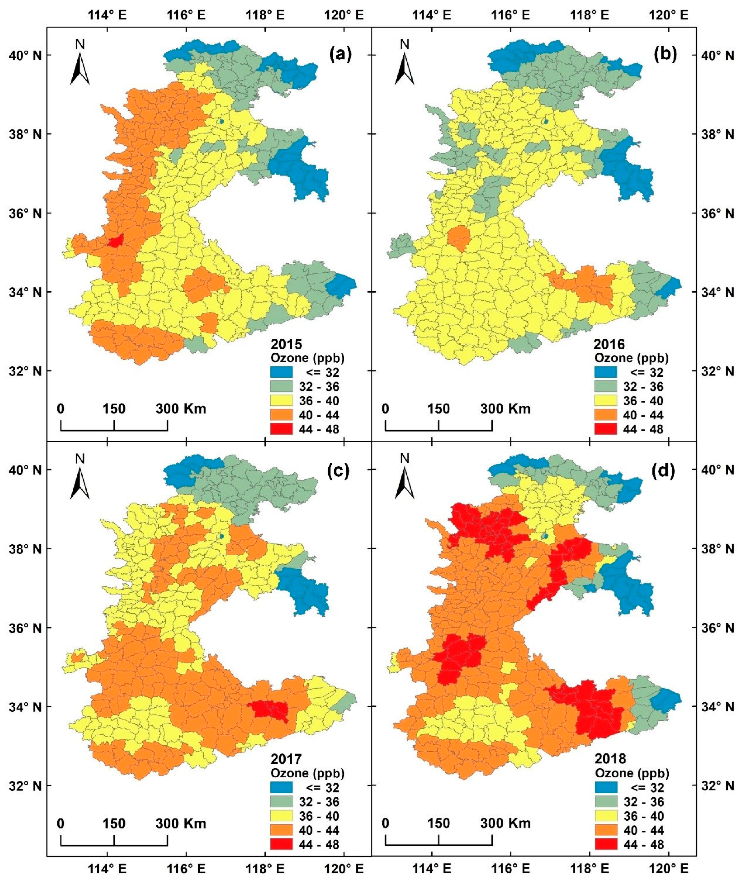
3.2. Spatio-Temporal Disparities in AOT40

The AOT40 during the winter wheat growing season were 5.53, 3.90, 5.17, and 6.70 ppm h for the years 2015, 2016, 2017, and 2018, respectively. Figure 3 shows that the county-level AOT40 clearly had spatial and temporal differences during this period. In general, the AOT40 was lower in the north and east than the south and west at the county scale, respectively. The AOT40 in 321 counties varied from 0.45 to 8.51 ppm h in 2015, from 0.76 to 6.69 ppm h in 2016, from 1.28 to 7.91 ppm h in 2017, and from 1.2 to 10.76 ppm h in 2018. In 2015, the county-level AOT40 was lower than 4.5 ppm h in the east and was higher than 6.5 ppm h in the west. The county-level AOT40 significantly increased in most parts of the NCP from 2016 to 2018. By 2018, the county-level AOT40 was above 6.5 ppm h at most regions of the NCP.

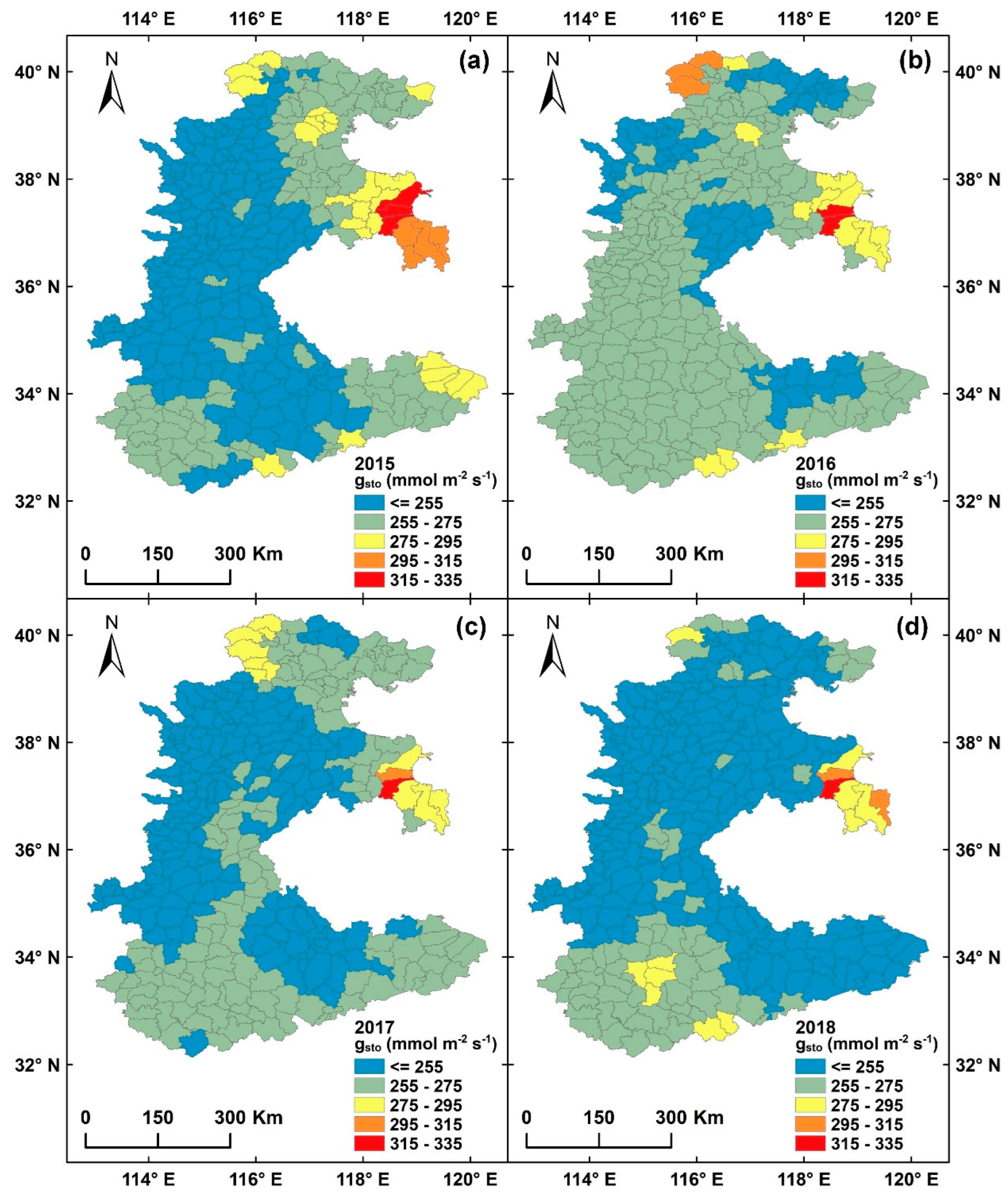
3.3. Spatio-Temporal Fluctuation of g_sto and POD₁₂

The g_sto was 253.75, 261.31, 248.86, and 248.98 mmol m⁻² s⁻¹ in the growing season of the years 2015, 2016, 2017, and 2018, respectively. The county-level g_sto from 2015 to 2018 clearly had spatial and temporal differences. From 2015 to 2018, the county-level relatively high g_sto (>295 mmol m⁻²s⁻¹) was mainly located in the east and north (Figure 4). The county-level g_sto was less than 275 mmol m⁻² s⁻¹ in most regions of the NCP during 2015–2018.

The POD₁₂ was 1.93, 1.52, 1.39, and 2.29 mmol m⁻² during the winter wheat growing season in 2015, 2016, 2017, and 2018, respectively. The county-level POD₁₂ had clear spatio-temporal variations from 2015 to 2018 (Figure 5). In general, the POD₁₂ in southern counties was higher than that in northern counties. The POD₁₂ clearly decreased year by year from 2015 to 2017. In 2017, the POD₁₂ was lower than 2.0 mmol m⁻² in most counties. In contrast, the county-level POD₁₂ was higher than 2.0 mmol m⁻² in most regions of the NCP in 2018.

3.4. Winter Wheat Yield Loss and Economic Reduction

The WRYLs based on AOT40 were 11.3% in 2015, 8.0% in 2016, 10.6% in 2017, and 13.7% in 2018. The county-level WRYLAOT40 was lower in the north than in the south from 2015 to 2018 (Figure 6). The range of WRYLAOT40 was 0.9–17.5%, 1.6–13.7%, 2.6–16.2%, and 2.5–22.1% for the years 2015, 2016, 2017, and 2018, respectively. In 2015, the county-level WRYLAOT40 was higher than 15% in the west and lower than 10% in the east (Figure 6a). During 2016–2018, the WRYLAOT40 clearly increased year by year at the county level.

The WRYLs estimated using POD₁₂ were 15.8%, 12.5%, 11.4%, and 18.8% for the years 2015, 2016, 2017, and 2018, respectively. Figure 7 shows that the county-level WRYLPOD₁₂ clearly had spatio-temporal variations from 2015 to 2018. In general, the WRYLPOD₁₂ in southern counties was higher than in the north. In 2015–2017, the WRYLPOD₁₂ clearly decreased year by year at the county scale. In 2017, the WRYLPOD₁₂ was lower than 15% in most counties. In 2018, however, the county-level WRYLPOD₁₂ was higher than 15% in most regions of the NCP and reached 25% or higher in the south.

The four-year mean WP, WPLAOT40, and WPLPOD₁₂ during 2015–2018 were 7572.8 × 104, 1022.7 × 104, and 1465.1 × 104 metric tons, respectively. The annual mean WPLAOT40 and WPLPOD₁₂ make up 13.5% and 19.4% of the annual average WP, respectively, and the annual average economic reduction using AOT40 (WELAOT40) and POD₁₂ (WELPOD₁₂) were USD 3.7 and 5.3 billion, respectively. The WPLAOT40 and WPLPOD₁₂ were 10.7 and 17.2 million metric tons in 2015, 7.3 and 12.9 million metric tons in 2016, 10.1 and 10.8 million metric tons in 2017, and 12.8 and 17.7 million metric tons in 2018. The production losses resulted in WELAOT40 and WELPOD₁₂ of USD 4.0 and 6.5 billion in 2015, USD 2.6 and 4.6 billion in 2016, USD 3.5 and 3.8 billion in 2017, and USD 4.5 and 6.2 billion in 2018, respectively. Results showed that WPL and WEL estimated by AOT40 were both lower than POD₁₂, and suggested similar inter-annual fluctuation (Figure 8). Figures S2–S5 show the spatio-temporal variation in county-level WPL and WEL based on AOT40 and POD₁₂ from 2015 to 2018, and Figure S6 (Tukey’s HSD test) illustrates the significance levels of the differences between WPL, WEL, and WP.

4. Discussion

In recent years, in China, surface O₃ has clearly increased annually, even as particulate matter pollution has decreased [3,40]. Surface O₃ concentration has exceeded 40 ppb in many regions of China [4,6,22,26]. Previous studies have shown that increasing O₃ concentrations reduces crop yield [4,22]. Some studies had estimated the effect of ground-level O₃ pollution on the yield of crops including wheat, rice, and maize [4,18]. However, previous studies were mainly based on the exposure-AOT40 metric using the data from relatively few urban monitoring stations [7,18,26]. The present study estimated the winter wheat yield loss and economic reduction based on the response relationships of flux and exposure using county-level O₃ and meteorological data simulated by WRF-Chem.

Results showed that the annual average AOT40 and WRYLAOT40 of the NCP was 5.32 ppm h and 10.9%, respectively, with clear spatio-temporal disparities. The mean AOT40 was reported to be 5.8 and 6.3 ppm h by Tang et al. [41] and Feng et al. [5], respectively. Some studies have estimated wheat yield losses using surface O₃ data from urban areas [17], but urban areas and rural areas are different; only rural data are relevant for estimating impacts on wheat growing. Using O₃ concentrations in urban areas cannot produce accurate estimates of wheat yield reduction due to O₃ [42,43,44,45]. WRF-Chem captures the differences in surface O₃ in urban and rural regions and thus, is more reliable for estimating impacts on wheat production [9].

Previous studies mainly estimated wheat yield reduction using O₃ exposure functions [9,18], without considering the crop growth environment. Some flux-based O₃ metrics (e.g., POD_y) had been developed to calculate the wheat production reduction in China and Europe [15,16,24,46] because assessment using flux-based POD_y was more accurate than exposure-based AOT40 at the regional scale.

In this study, the annual mean POD₁₂ and WRYLPOD₁₂ were found to be 1.78 mmol m⁻² and 14.6% over the NCP for the years 2015–2018, respectively. The mean POD₁₂ reported by previous studies for the NCP was about 3 mmol m⁻² [5,41]. These studies estimated wheat yield reduction using the O₃ and meteorological data at the provincial level [5,41] and without considering stomatal uptake. These two factors led to some uncertainty as to the accuracy of the assessment results.

Only two studies have used the same O₃ dose metrics (AOT40 and POD₁₂) to estimate the WRYL in China (

Table 3. WRYL using AOT40 and POD₁₂ metrics.

Metrics	Feng et al. [5]	Tang et al. [41]	This Study
AOT40	17.6%	11.9%	10.9%
POD12	10.4%	14.8%	14.6%

). Tang et al. [41] reported that the WRYL using POD₁₂ was around 1.2 times that based on AOT40. Similarly, in this study of the NCP, the WRYL based on POD₁₂ was 1.3 times that based on AOT40. The deviation of WRYL by Tang et al. [41] at a national scale from that in this study may be attributed to using the county-level data. However, Feng et al.’s [5] calculation of the WRYL over China based on POD₁₂ was about 0.6 times that of using AOT40. The difference between Feng et al. [5] and this study is likely because they used sparse monitoring data, which cannot capture well the local meteorological conditions.

Although similar spatial and temporal variations in winter wheat yield loss were observed using both AOT40 and POD₁₂, this study still has certain limitations. First, in addition to the anthropogenic emission inventory, previous studies have established that meteorological conditions also have a direct and important impact on the accuracy of O₃ simulation [40,47,48]. Therefore, the accuracy of simulating meteorological variables affects the accuracy of POD₁₂. Second, the wheat growing areas of the NCP is very large, and the cultivars grown were probably developed specifically for each region, so there could be genetic differences in dose responses for different cultivars [49]. In order to make more accurate assessments and predictions about the impact of O₃ on vital crops, we recommend that the following efforts be undertaken immediately: (1) collect stomatal conductance data for specific cultivars that are grown as the main crops in China such as the temperature and soil properties and (2) develop higher-resolution air pollutant inventories for the accurate high-resolution spatial and temporal modeling of O₃ concentrations and for the accurate simulation of meteorological conditions by climate models. Additionally, we recommend implementing a range of effective measures to protect winter wheat yields, which will enhance food security, for instance, as follows: (1) develop cultivars with improved ozone tolerance; (2) adopt strategies to control ozone pollution, such as reducing ozone precursors during the critical growth stages of winter wheat [50]; and (3) promote advancements in agricultural practices, green technologies, and environmental protection against industrial pollution, among other initiatives.

5. Conclusions

In this study, we used WRF-Chem to simulate O₃ and meteorological data for calculating the AOT40 and POD₁₂ during the winter wheat growing season from 2015 to 2018 in China and specifically over the NCP. Results show that the mean WRYL over the NCP for the years 2015–2018 based on AOT40 and POD₁₂ was 10.9% and 14.6%, respectively. The WPL and WEL induced by surface O₃ levels over the NCP from 2015 to 2018 were 12.4 million metric tons and USD 4.5 billion, respectively. Our findings indicate that in the NCP, the POD₁₂ index is more reliable than AOT40 for assessing ozone-induced yield losses in winter wheat. This discrepancy is likely due to local climatic factors, such as temperature and humidity, which reduce AOT40’s sensitivity. To maintain winter wheat productivity in the NCP, it is essential to consider breeding for ozone tolerance, as well as implementing effective measures to control surface ozone pollution, especially during the critical growth stages of winter wheat.

References

1. Wang, P.; Chen, Y.; Hu, J.; Zhang, H.; Ying, Q. Attribution of Tropospheric Ozone to NOx and VOC Emissions: Considering Ozone Formation in the Transition Regime. Environ. Sci. Technol. 2019, 53, 1404–1412. [Google Scholar] [CrossRef]
2. Gaudel, A.; Cooper, O.; Chang, K.; Bourgeois, I.; Ziemke, J.; Strode, S.; Oman, L.; Sellitto, P.; Nedelec, P.; Blot, R.; et al. Aircraft observations since the 1990s reveal increases of tropospheric ozone at multiple locations across the Northern Hemisphere. Sci. Adv. 2020, 6, eaba8272. [Google Scholar] [CrossRef] [PubMed]
3. Wang, T.; Song, H.; Wang, F.; Zhai, S.; Han, Z.; Wang, D.; Li, X.; Zhao, H.; Ma, R.; Zhang, G. Hysteretic effects of meteorological conditions and their interactions on particulate matter in Chinese cities. J. Clean. Prod. 2020, 274, 122926. [Google Scholar] [CrossRef]
4. Dong, C.; Gao, R.; Zhang, X.; Li, H.; Wang, W.; Xue, L. Assessment of O3-induced crop yield losses in northern China during 2013–2018 using high-resolution air quality reanalysis data. Atmos. Environ. 2021, 259, 118527. [Google Scholar] [CrossRef]
5. Feng, Z.; Kobayashi, K.; Li, P.; Xu, Y.; Tang, H.; Guo, A.; Paoletti, E.; Calatayud, V. Impacts of current ozone pollution on wheat yield in China as estimated with observed ozone, meteorology and day of flowering. Atmos. Environ. 2019, 217, 116945. [Google Scholar] [CrossRef]
6. Cheng, L.; Wang, S.; Gong, Z.; Li, H.; Yang, Q.; Wang, Y. Regionalization based on spatial and seasonal variation in ground-level ozone concentrations across China. J. Environ. Sci. 2018, 67, 179–190. [Google Scholar] [CrossRef]
7. Zhao, H.; Zheng, Y.; Wu, X. Assessment of yield and economic losses for wheat and rice due to ground-level O3 exposure in the Yangtze River Delta, China. Atmos. Environ. 2018, 191, 241–248. [Google Scholar] [CrossRef]
8. Ghamghami, M.; Beiranvand, J.P. Rainfed crop yield response to climate change in Iran. Reg. Environ. Chang. 2022, 22, 3. [Google Scholar] [CrossRef]
9. Wang, T.; Zhang, L.; Zhou, S.; Zhang, T.; Zhai, S.; Yang, Z.; Wang, D.; Song, H. Effects of ground-level ozone pollution on yield and economic losses of winter wheat in Henan, China. Atmos. Environ. 2021, 262, 118654. [Google Scholar] [CrossRef]
10. Agathokleous, E.; Feng, Z.; Oksanen, E.; Sicard, P.; Wang, Q.; Saitanis, C.; Araminiene, V.; Blande, J.; Hayes, F.; Calatayud, V.; et al. Ozone affects plant, insect, and soil microbial communities: A threat to terrestrial ecosystems and biodiversity. Sci. Adv. 2020, 6, eabc1176. [Google Scholar] [CrossRef]
11. Cooper, O.; Parrish, D.; Ziemke, J.; Balashov, N.; Cupeiro, M.; Galbally, I.; Gilge, S.; Horowitz, L.; Jensen, N.; Lamarque, J.; et al. Global distribution and trends of tropospheric ozone: An observation-based review. Elementa 2014, 2, 000029. [Google Scholar] [CrossRef]
12. Peng, J.; Shang, B.; Xu, Y.; Feng, Z.; Pleijel, H.; Calatayud, V. Ozone exposure- and flux-yield response relationships for maize. Environ. Pollut. 2019, 252, 1–7. [Google Scholar] [CrossRef]
13. Mills, G.; Sharps, K.; Simpson, D.; Pleijel, H.; Broberg, M.; Uddling, J.; Jaramillo, F.; Davies, W.; Dentener, F.; Van den Berg, M.; et al. Ozone pollution will compromise efforts to increase global wheat production. Glob. Chang. Biol. 2018, 24, 3560–3574. [Google Scholar] [CrossRef]
14. Zhang, W.; Feng, Z.; Wang, X.; Liu, X.; Hu, E. Quantification of ozone exposure and stomatal uptake- yield response relationships for soybean in Northeast China. Sci. Total Environ. 2017, 599, 710–720. [Google Scholar] [CrossRef]
15. Feng, Z.; Tang, H.; Uddling, J.; Pleijel, H.; Kobayashi, K.; Zhu, J.; Oue, H.; Guo, W. A stomatal ozone flux–response relationship to assess ozone-induced yield loss of winter wheat in subtropical China. Environ. Pollut. 2012, 164, 16–23. [Google Scholar] [CrossRef]
16. Pleijel, H.; Danielsson, H.; Emberson, L.; Ashmore, M.; Mills, G. Ozone risk assessment for agricultural crops in Europe: Further development of stomatal flux and flux–response relationships for European wheat and potato. Atmos. Environ. 2007, 41, 3022–3040. [Google Scholar] [CrossRef]
17. Hu, T.; Liu, S.; Xu, Y.; Feng, Z.; Calatayud, V. Assessment of O3-induced yield and economic losses for wheat in the North China Plain from 2014 to 2017, China. Environ. Pollut. 2020, 258, 113828. [Google Scholar] [CrossRef]
18. Zhao, H.; Zheng, Y.; Zhang, Y.; Li, T. Evaluating the effects of surface O3 on three main food crops across China during 2015–2018. Environ. Pollut. 2020, 258, 113794. [Google Scholar] [CrossRef]
19. Kumari, S.; Lakhani, A.; Kumari, K. First observation-based study on surface O3 trend in Indo-Gangetic Plain: Assessment of its impact on crop yield. Chemosphere 2020, 255, 126972. [Google Scholar] [CrossRef]
20. Zhu, X.; Feng, Z.; Sun, T.; Liu, X.; Tang, H.; Zhu, J.; Guo, W.; Kobayashi, K. Effects of elevated ozone concentration on yield of four Chinese cultivars of winter wheat under fully open-air field conditions. Glob. Chang.Biol. 2011, 17, 2697–2706. [Google Scholar] [CrossRef]
21. Mills, G.; Buse, A.; Gimeno, B.; Bermejo, V.; Holland, M.; Emberson, L.; Pleijel, H. A synthesis of AOT40-based response functions and critical levels for ozone for agricultural and horticultural crops. Atmos. Environ. 2007, 41, 2630–2643. [Google Scholar] [CrossRef]
22. Wang, T.; Wang, F.; Song, H.; Zhou, S.; Ru, X.; Zhang, H. Maize yield reduction and economic losses caused by ground-level ozone pollution with exposure- and flux-response relationships in the North China Plain. J. Environ. Manag. 2022, 324, 116379. [Google Scholar] [CrossRef]
23. LRTAP. Mapping Critical Levels for Vegetation, Chapter III of Manual on Methodologies and Criteria for Modelling and Mapping Critical Loads and Levels and Air Pollution Effects, Risks and Trends. UNECE Convention on Long-Range Transboundary Air Pollution. 2017. Available online: www.icpmapping.org (accessed on 7 October 2024).
24. Mills, G.; Sharps, K.; Simpson, D.; Pleijel, H.; Frei, M.; Burkey, K.; Emberson, L.; Uddling, J.; Broberg, M.; Feng, Z.; et al. Closing the global ozone yield gap: Quantification and cobenefits for multistress tolerance. Glob. Chang. Biol. 2018, 24, 4869–4893. [Google Scholar] [CrossRef]
25. Tang, H.; Pang, J.; Zhang, G.; Takigawa, M.; Liu, G.; Zhu, J.; Kobayashi, K. Mapping ozone risks for rice in China for years 2000 and 2020 with flux-based and exposure-based doses. Atmos. Environ. 2014, 86, 74–83. [Google Scholar] [CrossRef]
26. Feng, Z.; Hu, T.; Tai, A.; Calatayud, V. Yield and economic losses in maize caused by ambient ozone in the North China Plain (2014–2017). Sci. Total Environ. 2020, 722, 137958. [Google Scholar] [CrossRef]
27. Danh, N.; Huy, L.; Oanh, N. Assessment of rice yield loss due to exposure to ozone pollution in Southern Vietnam. Sci. Total Environ. 2016, 566, 1069–1079. [Google Scholar] [CrossRef]
28. Song, H.; Wang, K.; Zhang, Y.; Hong, C.; Zhou, S. Simulation and evaluation of dust emissions with WRF-Chem (v3.7.1) and its relationship to the changing climate over East Asia from 1980 to 2015. Atmos. Environ. 2017, 167, 511–522. [Google Scholar] [CrossRef]
29. Zaveri, R.; Peters, L. A new lumped structure photochemical mechanism for large-scale applications. J. Geophys. Res. 1999, 104, 30387–30415. [Google Scholar] [CrossRef]
30. Madronich, S. Intercomparison of NO2 photodissociation and u.v. radiometer measurements. Atmos. Environ. 1987, 21, 569–578. [Google Scholar] [CrossRef]
31. Zaveri, R.A.; Easter, R.C.; Fast, J.D.; Peters, L.K. Model for simulating aerosol interactions and chemistry (MOSAIC). J. Geophys. Res. 2008, 113, D13204. [Google Scholar] [CrossRef]
32. Tilmes, S.; Lamarque, J.; Emmons, L.; Kinnison, D.; Ma, P.; Liu, X.; Ghan, S.; Bardeen, C.; Arnold, S.; Deeter, M.; et al. Description and evaluation of tropospheric chemistry and aerosols in the community earth system model (CESM1.2). Geosci. Model Dev. 2015, 8, 1395–1426. [Google Scholar] [CrossRef]
33. Zhang, Q.; Streets, D.; Carmichael, G.; He, K.; Huo, H.; Kannari, A.; Klimont, Z.; Park, I.; Reddy, S.; Fu, J.; et al. Asian emissions in 2006 for the NASA INTEX-B mission. Atmos. Chem. Phys. 2009, 9, 5131–5153. [Google Scholar] [CrossRef]
34. Wiedinmyer, C.; Yokelson, R.; Gullett, B. Global Emissions of Trace Gases, Particulate Matter, and Hazardous Air Pollutants from Open Burning of Domestic Waste. Environ. Sci. Technol. 2014, 48, 9523–9530. [Google Scholar] [CrossRef]
35. Guenther, A.; Karl, T.; Harley, P.; Wiedinmyer, C.; Palmer, P.; Geron, C. Estimates of global terrestrial isoprene emissions using MEGAN (Model of Emissions of Gases and Aerosols from Nature). Atmos. Chem. Phys. 2006, 6, 3181–3210. [Google Scholar] [CrossRef]
36. Pleijel, H. A Suggestion of a Simple Transfer Function for the Use of Ozone Monitoring Data in Dose-response Relationships Obtained Using Open-Top Chambers. Water Air Soil Pollut. 1998, 102, 61–74. [Google Scholar] [CrossRef]
37. Emberson, L.; Ashmore, M.; Cambridge, H.; Simpson, D.; Tuovinen, J. Modelling stomatal ozone flux across Europe. Environ. Pollut. 2000, 109, 403–413. [Google Scholar] [CrossRef]
38. Emberson, L.; Wieser, G.; Ashmore, M. Modelling of stomatal conductance and ozone flux of Norway spruce: Comparison with field data. Environ. Pollut. 2000, 109, 393–402. [Google Scholar] [CrossRef]
39. Feng, Z.; Xu, Y.; Kobayashi, K.; Dai, L.; Zhang, T.; Agathokleous, E.; Calatayud, V.; Paoletti, E.; Mukherjee, A.; Agrawal, M.; et al. Ozone pollution threatens the production of major staple crops in East Asia. Nat. Food 2022, 3, 47–56. [Google Scholar] [CrossRef]
40. Liu, P.; Song, H.; Wang, T.; Wang, F.; Li, X.; Miao, C.; Zhao, H. Effects of meteorological conditions and anthropogenic precursors on ground-level ozone concentrations in Chinese cities. Environ. Pollut. 2020, 262, 114366. [Google Scholar] [CrossRef]
41. Tang, H.; Takigawa, M.; Liu, G.; Zhu, J.; Kobayashi, K. A projection of ozone-induced wheat production loss in China and India for the years 2000 and 2020 with exposure-based and flux-based approaches. Glob. Chang. Biol. 2013, 19, 2739–2752. [Google Scholar] [CrossRef]
42. Sicard, P.; Serra, R.; Rossello, P. Spatiotemporal trends in ground-level ozone concentrations and metrics in France over the time period 1999–2012. Environ. Res. 2016, 149, 122–144. [Google Scholar] [CrossRef]
43. Sicard, P.; Anav, A.; De Marco, A.; Paoletti, E. Projected global ground-level ozone impacts on vegetation under different emission and climate scenarios. Atmos. Chem. Phys. 2017, 17, 12177–12196. [Google Scholar] [CrossRef]
44. Guerreiro, C.; Foltescu, V.; de Leeuw, F. Air quality status and trends in Europe. Atmos. Environ. 2014, 98, 376–384. [Google Scholar] [CrossRef]
45. Xu, J.; Zhang, X.; Xu, X.; Zhao, X.; Meng, W.; Pu, W. Measurement of Surface Ozone and its Precursors in Urban and Rural Sites in Beijing. Procedia Earth Planet. Sci. 2011, 2, 255–261. [Google Scholar] [CrossRef]
46. Mills, G.; Hayes, F.; Simpson, D.; Emberson, L.; Norris, D.; Harmens, H.; Buker, P. Evidence of widespread effects of ozone on crops and (semi-)natural vegetation in Europe (1990–2006) in relation to AOT40-and flux-based risk maps. Glob. Chang. Biol. 2011, 17, 592–613. [Google Scholar] [CrossRef]
47. Chen, Z.; Zhuang, Y.; Xie, X.; Chen, D.; Cheng, N.; Yang, L.; Li, R. Understanding long-term variations of meteorological influences on ground ozone concentrations in Beijing during 2006–2016. Environ. Pollut. 2019, 245, 29–37. [Google Scholar] [CrossRef]
48. Han, H.; Liu, J.; Shu, L.; Wang, T.; Yuan, H. Local and synoptic meteorological influences on daily variability of summertime surface ozone in eastern China. Atmos. Chem. Phys. 2020, 20, 203–222. [Google Scholar] [CrossRef]
49. Guarin, J.R.; Jägermeyr, J.; Ainsworth, E.A.; Oliveira, F.A.; Asseng, S.; Boote, K.; Elliott, J.; Emberson, L.; Foster, I.; Hoogenboom, G.; et al. Modeling the effects of tropospheric ozone on the growth and yield of global staple crops with DSSAT v4. 8.0. Geosci. Model Dev. 2024, 17, 2547–2567. [Google Scholar] [CrossRef]
50. Agathokleous, E.; Frei, M.; Knopf, O.M.; Muller, O.; Xu, Y.; Nguyen, T.H.; Gaiser, T.; Liu, X.; Liu, B.; Saitanis, C.J.; et al. Adapting crop production to climate change and air pollution at different scales. Nat. Food 2023, 4, 854–865. [Google Scholar] [CrossRef]
Figure 1. Maps of the domains used in WRF-Chem. (a) D01, Domain 1, representing all of China. (b) D02, Domain 2, showing locations of monitoring stations. In both maps, the shaded area represents the North China Plain (NCP).
Agronomy 14 02326 g001
Figure 2. Spatial distributions of mean daytime (08:00–18:00) surface O3 during winter wheat growing season ((a) 2015; (b) 2016; (c) 2017; (d) 2018).
Agronomy 14 02326 g002
Figure 3. County-level AOT40 in the winter wheat growing season over the NCP ((a) 2015; (b) 2016; (c) 2017; (d) 2018).
Agronomy 14 02326 g003
Figure 4. County-scale gsto during the winter wheat growing seasons over the NCP ((a) 2015; (b) 2016; (c) 2017; (d) 2018).
Agronomy 14 02326 g004
Figure 5. County-scale POD12 in the winter wheat growing seasons over the NCP ((a) 2015; (b) 2016; (c) 2017; (d) 2018).
Agronomy 14 02326 g005
Figure 6. County-scale winter wheat relative yield reduction based on AOT40 ((a) 2015; (b) 2016; (c) 2017; (d) 2018).
Agronomy 14 02326 g006
Figure 7. County-level winter wheat relative yield reduction based on POD12 ((a) 2015; (b) 2016; (c) 2017; (d) 2018).
Agronomy 14 02326 g007
Figure 8. Annual production loss of winter wheat (WPL), production of winter wheat (WP), and winter wheat economic loss (WEL) of the NCP during 2015–2018.
Agronomy 14 02326 g008