Article

Inversion of Crop Water Content Using Multispectral Data and Machine Learning Algorithms in the North China Plain

1
College of Agronomy, Henan Agricultural University, Zhengzhou 450002, China
2
College of Water Resource and Architecture Engineering, Tarim University, Aral 843300, China
3
Institute of Farmland Irrigation, Chinese Academy of Agricultural Sciences, Key Laboratory of Crop Water Use and Regulation, Ministry of Agriculture and Rural Affairs, Xinxiang 453002, China
4
Institute of Quantitative Remote Sensing & Smart Agriculture, School of Surveying and Land Information Engineering, Henan Polytechnic University, Jiaozuo 454000, China
*
Authors to whom correspondence should be addressed.
Agronomy 2024, 14(10), 2361; https://doi.org/10.3390/agronomy14102361
Submission received: 4 September 2024 / Revised: 10 October 2024 / Accepted: 11 October 2024 / Published: 13 October 2024
(This article belongs to the Special Issue Plant–Water Relationships for Sustainable Agriculture)

Abstract

:
(1) Background: Accurate inversion of crop water content is key to making an intelligent irrigation decision. However, little effort has been devoted to accurately estimating the crop water content of winter wheat in the North China Plain. (2) Method: The crop water content of winter wheat was measured at jointing, flowering and grain-filling stages, respectively. UAV-based multispectral remote sensing images were used to calculate thirteen vegetation indices, including SAVI, EVI, R-M, NDRE, OSAVI, GOSAVI, REOSAVI, GBNDVI, NDVI, RVI, DVI, GNDVI, and TVI. Five machine learning (ML) algorithms (i.e., MLR, RF, PLSR, ElasticNet, and ridge regression) were adopted to estimate the crop water content of winter wheat at the three growth stages. The benchmark datasets, which include CWC as well as vegetation indices calculated based on spectral indices, were adopted to validate the performance of the ML models. (3) Results: The correlation coefficients ranged from 0.64 to 0.82 at different growth stages. The optimal vegetation indices were GNDVI for the jointing stage, NDRE for the flowering and the grain-filling stage, respectively. Among the five machine learning methods, random forest (RF) showed the best performance across the three growth stages, with its coefficient of determination (R2) of 0.80, or an increase by 20.1% than those of other models. In addition, the RMSE and RPD of the RF model at the flowering stage were 3.00% and 2.01, which significantly outperformed other models and growth stages. (4) Conclusion: This study may provide theoretical support and technical guidance for monitoring current water status in wheat crops, which is useful to develop a precise irrigation prescription map for local farmers. (5) Limitation: The main limitation of this study is that the sample size is relatively small and may not fully reflect the characteristics of the target groups. At the same time, subjectivity and bias may exist in the data collection, which may have a certain impact on the accuracy of the results. Future studies could consider expanding sample sizes and improving data collection methods to overcome these limitations.

1. Introduction

Crop water content (CWC) is a key element for diagnosing crop water deficiencies [1]. Obtaining timely and accurate information on CWC is crucial for the advancement of precision agriculture [2]. Traditional methods for estimating CWC typically involve destructive sampling and direct measurement using soil water monitors, which are labor intensive, time consuming, and limited in spatial coverage, making them unsuitable for rapid monitoring [3]. Therefore, developing simpler and more accurate methods for estimating CWC has become a hot topic worldwide.
With advances in remote sensing technology, unmanned aerial vehicles (UAVs) equipped with multispectral sensors have emerged as a promising tool for efficiently monitoring crop conditions over large areas [4]. Feng et al. (2022) used UAVs equipped with RGB and hyperspectral cameras to monitor CWC of winter wheat during the critical periods and found that the flowering stage was the best period for monitoring CWC [5]. Pei et al. (2017) used UAV hyperspectral images to reflect the growth of wheat at different stages and identified comprehensive growth index (CGI) as one of the best indices for monitoring CWC of wheat plants [6]. Multispectral remote sensing captures data across different wavelengths, enabling the calculation of various vegetation indices that can be correlated with CWC [7]. However, the effectiveness of these indices in estimating CWC varies across different crop growth stages [8]. Therefore, it is necessary to identify the most relevant vegetation indices, thus improving the accuracy of CWC estimation.
Recently, significant progress has been made in the areas of CWC monitoring using satellite and ground-based remote sensing [9,10,11]. Han et al. (2011) studied the correlation between canopy reflectance spectra and CWC of winter wheat and found that the spectral reflectance in the 780–805 nm range best indicated the changes in CWC status [12]. Wang et al. (2013) developed various vegetation indices and normalized those indices using all possible pairwise combinations of spectral bands within the 350–2500 nm range, achieving high accuracy in diagnosing CWC of cotton in Northwest China [13]. In recent years, machine learning models have been adopted to enhance the accuracy of CWC estimation [14,15]. As an example, Zhang et al. (2014) developed an innovative method for wheat CWC detection using near-infrared photodetectors and a support vector machine, demonstrating an effective approach for non-destructive and rapid detection of wheat CWC [16]. Habure et al. (2018) indicated that the reflectance of winter wheat canopies decreased with CWC, in which the indices using wavelengths at 661 nm and 771 nm performed best in CWC estimation [17]. Ndlovu et al. (2021) found that random forest (RF) was one of the best algorithms to estimate the equivalent water thickness (EWT), fuel moisture content (FMC) and specific leaf area (SLA) of maize leaves with significant results, and the root mean square error (RMSE) was as low as 3.13%, 1% and 3.48%, respectively [18]. Han et al. (2019) used the spectral features of Sentinel-2 remote sensing images to construct multiple optical vegetation indices and adopted grey correlation analysis method to select optimal vegetation indices combined with multiple linear regression modeling to retrieve wheat crop water content. The accuracy of the model in the validation phase was acceptable, with R = 0.632, RMSE = 0.021 and nRMSE = 19.65%, respectively [19].
In the field of UAV remote sensing, several notable studies have been conducted. Hassan-Esfahani et al. (2015) used UAV equipped with hyperspectral cameras to capture spectral images and accurately estimated surface soil moisture using artificial neural networks [20]. Chen et al. (2018) developed a method for rapidly acquiring large-scale CWC data using low-altitude UAV multispectral remote sensing and created an optimal model at the flowering stage of winter wheat [21]. Chen et al. (2018) established one of the optimal inversion models using multispectral UAV images to estimate various crop evapotranspiration (ETc) parameters of cotton, indicating the feasibility of large-scale ETc monitoring using UAV data [22]. To date, UAV remote sensing technologies offers significant advantages in CWC monitoring due to its easy mobility, wide adaptability, and high image resolution. This method is becoming increasingly important in precision agriculture, providing new solutions for monitoring crop water conditions [23]. Nevertheless, studies using machine learning algorithms and UAV multispectral remote sensing imagery to accurately estimate CWC in winter wheat remain limited in the North China Plain (NCP) [24].
In this study, high-resolution multispectral images of wheat canopies were captured at the jointing, flowering, and grain-filling stages, and various vegetation indices were calculated. Regression analysis was performed to establish relationships between CWC and the vegetation indices. After careful comparison of ten machine learning models’ performance in training and testing phases, we finally selected five specific machine learning models—multiple linear regression (MLR), random forest (RF), ridge regression, ElasticNet, and partial least squares regression (PLSR)—to achieve CWC estimation. We hypothesized that there were the best combinations of machine learning algorithms and vegetation indices that accurately estimated the CWC of winter wheat in the NCP. The objectives of this study were (I) to evaluate the performance of different vegetation indices and machine learning algorithms in estimating CWC in winter wheat at different growth stages, and (II) to identify the optimal combinations of vegetation indices and ML models for monitoring CWC at field scale. This study is of significance in providing valuable insights and practical tools for precision agriculture.

2. Materials and Methods

2.1. Site Description

A field experiment was carried out from October 2023 to June 2024, at the Qiliying Experimental Station, Xinxiang city, Henan province, China (35°08′ N, 113°45′ E, a.s.l. 81 m) (Figure 1). The experimental plots were irrigated with groundwater from wells with a depth of 50 m. The cropping system is a winter wheat–summer maize cropping rotation. The place has a continent temperate monsoon climate. The mean annual precipitation (1953–2023) is 603 mm, of which 35% occurs during the winter wheat growing season. The mean annual temperature is 14.1 °C. The annual evaporation is 1909 mm, annual sunshine hours are 2408 h, and the annual frost-free period is 201 d. The average solar radiation is about 4900 MJ m−2 y−1. The soil was classified as sandy loam soil (Table 1). The available soil N, P, K, and soil organic matter content were 43.1 mg kg−1, 15.2 mg kg−1, 126 mg kg−1, and 13.1 g kg−1, respectively.

2.2. Experimental Design

Winter wheat seeds (c.v. Bainong-4199) were sown on 15 October 2023 and harvested on 5 June 2024. The seeding rate was 225 kg ha−1, and sowing depth was 3–5 cm. Planting density was 4.5 × 10⁶ plants ha−1, with row spacing of 18 cm. The plot size was 12 m × 10 m, with a plot area of 120 m2. Three irrigation quotas and three nitrogen levels were designed and arranged in an incomplete randomized block design. Except an initial irrigation (45 mm) which was applied after sowing to aid seeds’ germination, irrigation quotas were set at 0, 30 and 60 mm per irrigation event at wintering (20 November 2023), jointing (20 March 2024), and flowering (21 April 2024) stages. Irrigation volumes were recorded using a flow meter (MIK-2000H Co., Ltd., Shanghai, China) installed on the main pipe of the micro-sprinkler system, with a flow rate of 3.0 L h−1. Phosphorus and potassium fertilizers were broadcast at the rate of 90 and 80 kg ha−1 as base fertilizer at sowing. Each treatment had three replicates, and thus, a total of 27 experimental plots were set up. All crops were managed using local government recommended practices, including uniform weeding, and pest control.

2.3. Data Collection and Processing

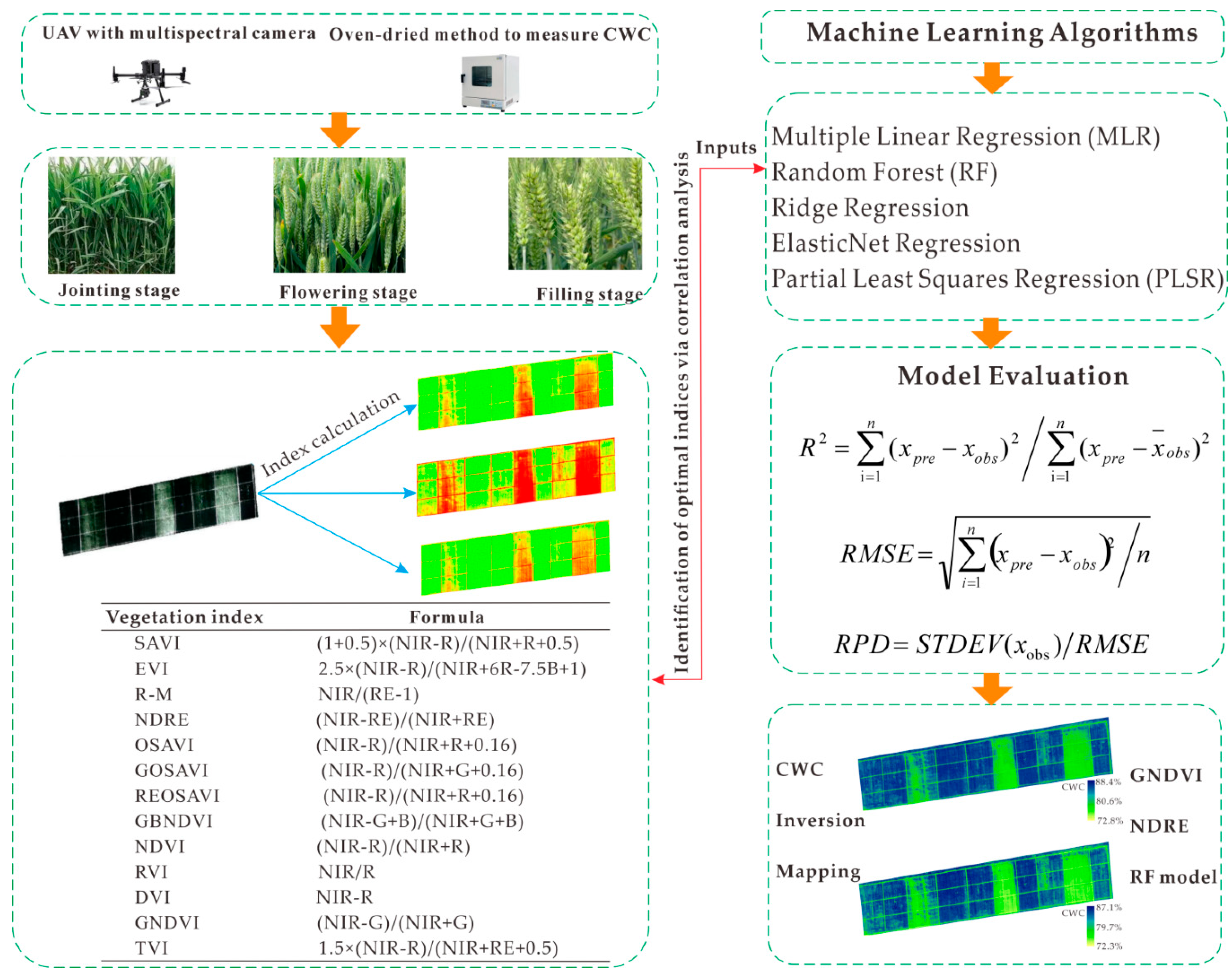
The DJI Matrice 300 UAV (DJI Technology Co., Ltd., Shenzhen, China) equipped with an MS600 Pro multispectral camera (Changguang Yusense Co., Ltd., Qingdao, China) was used for image acquisition. The UAV had a take-off weight of 9.0 kg, and a net payload of 5.5 kg. Two batteries were simultaneously used for the UAV, supporting it flying about 30 min per flight. The maximum communication distance was 5.0 km. Flight routes were pre-set to cover the entire experimental area. Images of wheat canopies were captured at the jointing (25 March 2024), flowering (16 April 2024), and grain-filling (12 May 2024) stages. The camera was a 6-band multispectral camera (Changguang Yusense Co., Ltd., Qingdao, China), which was mounted on a pan-tilt platform to capture smooth and clear photos in each flight. The six spectral bands were blue (450 nm), green (555 nm), red (660 nm), red edge 01 (720 nm), red edge 02 (750 nm), and near infrared (840 nm) (Table 2). In this study, red edge 01 data were mainly involved in the calculation of vegetation indices. Images were acquired between 11:00 and 14:00 with a solar altitude angle > 50° in sunny weather. The lens was positioned vertically downwards in each flight with a focal length of 25 mm. The flight height was set at 30 m, and the flight speed was set at 5 m s−1. The longitudinal overlap was 85%, and the lateral overlap was 75%, providing a ground resolution of 4.77 cm per pixel. The calibration system included an optical intensity sensor and a fixed reflectance calibration panel. The optical intensity sensor corrected for variations in external lighting that might affect the spectral images, while the fixed reflectance calibration panel was used for radiometric calibration, ensuring an accurate multispectral image. Raw remote sensing images were stitched together using Pix4D 4.5.6 mapper software (PIX4D, Lausanne, Switzerland). ENVI 5.6 software was used for band fusion and radiometric calibration of images. Reflectance values at sample points were extracted from the processed images using ArcMap 10.8. The reflectance values from the sampling points were used to analyze their correlation with crop water content (CWC, %). The UAV acquisition at the jointing, flowering, and filling stages, selection of vegetation indices, identification of prediction models, and model evaluation are shown in Figure 2.

2.4. Calculation of Vegetation Indices

The combination of reflectance of different bands was used to calculate various vegetation indices. It includes soil-adjusted vegetation index (SAVI), enhanced vegetation index (EVI), red edge model (R-M), normalized red edge vegetation index (NDRE), optimized soil-adjusted vegetation index (OSAVI), optimized green soil-adjusted vegetation index (GOSAVI), optimized red edge soil-adjusted vegetation index (REOSAVI), and normalized blue-green zone differential vegetation index (GBNDVI), normalized differential vegetation index (NDVI), proportional vegetation index (RVI), differential vegetation index (DVI), green normalized vegetation difference index (GNDVI), and triangular vegetation index (TVI) (Table 3). This process helped mitigate the effects of atmospheric, soil, and water background factors, thus enhancing the accuracy and reliability of the retrieval results. The above-mentioned vegetation indices were considered sensitive to changes in vegetation cover, growth conditions, and biomass, allowing them to accurately reflect the growth status and trends of vegetation. The indices were primarily calculated using Python 3.10, with the calculation formulas detailed in Table 3.

2.5. Measurement of Crop Water Content (CWC)

Wheat plants were sampled from 0.25 m × 0.25 m quadrats in each plot immediately after multispectral data collection. Accurate sampling positions were recorded for extracting point reflectance values. The samples were immediately brought to the laboratory to determine their fresh weight. They were separated and placed in an oven at 105 °C for 30 min to stop enzymatic activity and then oven-dried at 75 °C for 48 h until constant weight. Wheat CWC was measured after the dry weights were determined, which were served as the dependent variables in the regression analysis.
As a crucial factor indicating the plant’s water status, the percentage of CWC in wheat plants was calculated using the following equation:
C W C = m 1 m 2 m 1 × 100 % ,
where CWC is crop water content, expressed as a percentage (%), m1 is the fresh weight of the plant samples, measured in grams (g m−2), and m2 is the dry weight of the plant samples, measured in grams (g m−2).

2.6. Machine Learning Algorithms

Five machine learning models were used for CWC estimation: multiple linear regression (MLR), random forest (RF), ridge regression, ElasticNet regression, and partial least squares regression (PLSR). Each model was trained and tested to evaluate its performance in predicting CWC.

2.6.1. Multiple Linear Regression (MLR)

Multiple linear regression was a statistical method adopted to analyze the relationship between one dependent variable and multiple independent variables [37]. The goal of MLR was to create a predictive model that estimated the dependent variable from the given independent variables [38]. It was useful for understanding and quantifying the linear relationship between variables to estimate CWC based on a multiple linear relationship. The model estimated unbiasedly the regression coefficients through minimizing the sum of squared differences between predicted and observed values.

2.6.2. Random Forest (RF)

The random forest model was able to handle complex, non-linear relationships and interactions among features to predict CWC [39]. It was an ensemble learning method that constructed multiple decision trees during training and output the mode of the classes or mean prediction of the individual trees [40]. The model had the advantage of being robust to overfitting and was able to process large datasets with many features. In regression analysis, RF was shown to be effective in capturing interactions between different vegetation indices and CWC.

2.6.3. Ridge Regression

Ridge regression addressed multicollinearity among features and provided regularization to prevent overfitting [41]. It was a type of linear regression that included a penalty term (L2 regularization) to shrink the coefficients of the model [42]. It was shown useful when dealing with highly correlated features, helping to stabilize the coefficient estimates.

2.6.4. ElasticNet Regression

ElasticNet regression combined the properties of both Ridge and Lasso (L1 regularization) regression for feature selection and regularization [43]. The model used a linear model with both L1 and L2 penalties, allowing for variable selection and regularization [44]. It was shown effective when there were multiple features with potential redundancy, helping to improve model generalization.

2.6.5. Partial Least Squares Regression (PLSR)

The PLSR model reduced the dimensionality of data by projecting the predictor variables and the response variables into a lower-dimensional space [45]. The model found latent variables (components) that captured the maximum variance in the predictors and the response variables [46]. It was shown useful when dealing with high-dimensional data where features were highly collinear.

2.7. Dataset Description

Crop water content (CWC) is one of the important indices uses to reflect the water status of winter wheat, which is of great significance for guiding agricultural production, optimizing the irrigation scheme and increasing yield. As an important parameter in remote sensing technology, vegetation index can reflect crop growth state, water status and other information. By creating a dataset between the two indicators (i.e., CWC and vegetation indices), remote sensing data can be combined with CWC of winter wheat plants to achieve accurate monitoring and prediction of crop water status, providing scientific basis for agricultural production and precision irrigation.

2.8. Model Evaluation Metrics

Metrics such as coefficient of determination (R2), root mean square error (RMSE), and relative prediction deviation (RPD) were adopted to assess model accuracy. This methodology aimed to provide a robust approach for evaluating the performance of the models by comparing predicted CWC with actual field measurements. These metrics collectively provided a comprehensive view of the model’s performance, offering insights into the fit, accuracy, and precision of the predictions made by the model. Generally, R2 describes the proportion of variance in measured CWC explained by model predictions and was calculated using Equation (2):
R 2 = i = 1 n ( x p r e x o b s ) 2 / i = 1 n ( x p r e x ¯ o b s ) 2
where R2 was root mean square error; xpre and xobs were predicted and observed CWC values, respectively; x ¯ o b s was the average observed values; and n was the number of values evaluated.
The RMSE was used to investigate the differences between predicted and observed CWC values and was calculated using Equation (3):
R M S E = i = 1 n ( x p r e x o b s ) 2 / n
where RMSE was root mean square error; xpre and xobs were corresponding CWC values estimated based on model prediction and field observation, respectively; and n was the sample number. The smaller the RMSE values were, the more accurate the model prediction data turned out to be.
The RPD was used to indicate the reliability of model prediction data and was calculated using Equation (4):
R P D = S T D E V ( x o b s ) / R M S E
where RPD was relative prediction deviation; STDEV was the standard deviation of observed CWC values; RMSE was root mean square error; and xobs was observed CWC values. RPD ≥ 2.0 indicated predictions were reliable; 1.4 < RPD < 2.0 meant the data were feasible but needed to be improved; and RPD ≤ 1.4 indicated the data were unreliable [47].

2.9. Statistical Analysis

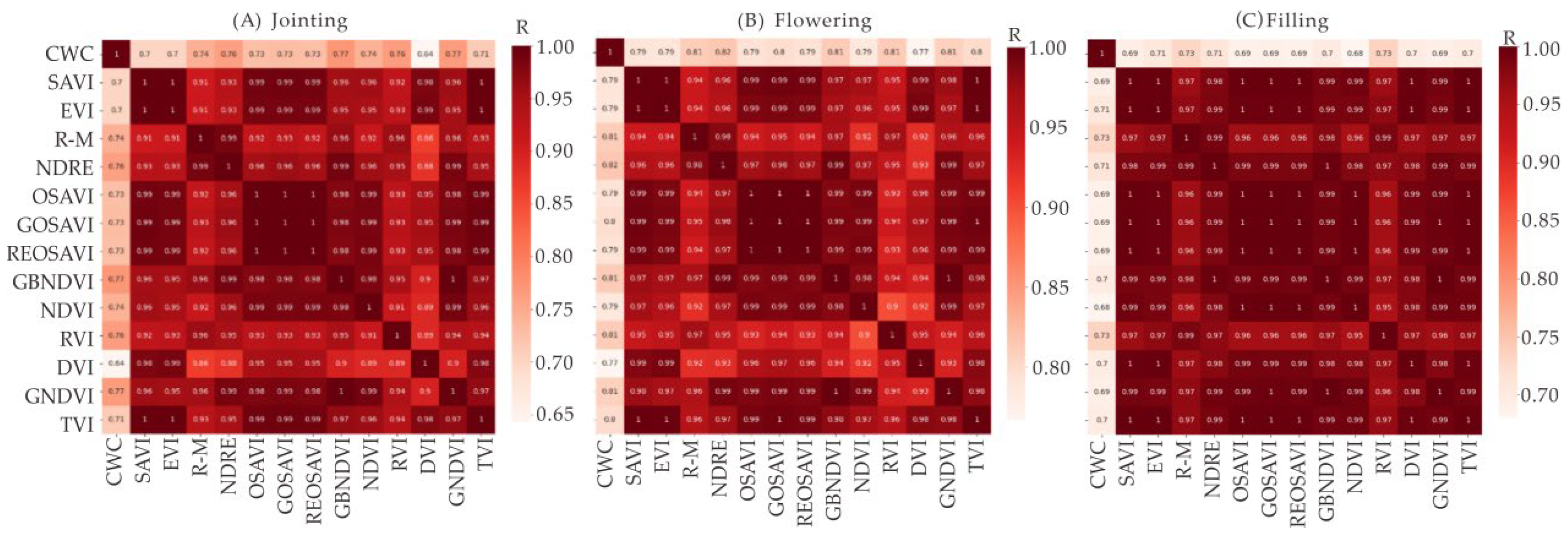
Pearson correlation analysis was conducted to evaluate the relationship between selected vegetation indices and CWC at the jointing, flowering, and filling growth stages of winter wheat. The analysis, performed using Python 3.10, displayed correlation values numerically, with higher values indicating stronger correlations and darker colors representing higher correlation strengths.

3. Results

3.1. Correlation Analysis between Vegetation Indices and CWC

Correlation coefficients (R) between vegetation indices and crop water content (CWC, %) varied across different growth stages (Figure 3). For example, GNDVI had the highest R value (0.77) with CWC at the jointing stage, while the index with the highest R (0.82) was NDRE at the flowering stage. The greatest R value was 0.71 for R-M and RVI indices at the grain-filling stage of winter wheat. Besides, R values for the rest vegetation indices were 0.75–0.80 at the flowering stage, consistently higher than those of the other growth stages. Generally, R values were highest at the flowering stage, intermediate at the jointing stage, and least at the grain-filling stage. This suggested that the flowering stage might be the most effective stage for CWC inversion using vegetation indices.

3.2. Vegetation Indices at the Flowering Stage

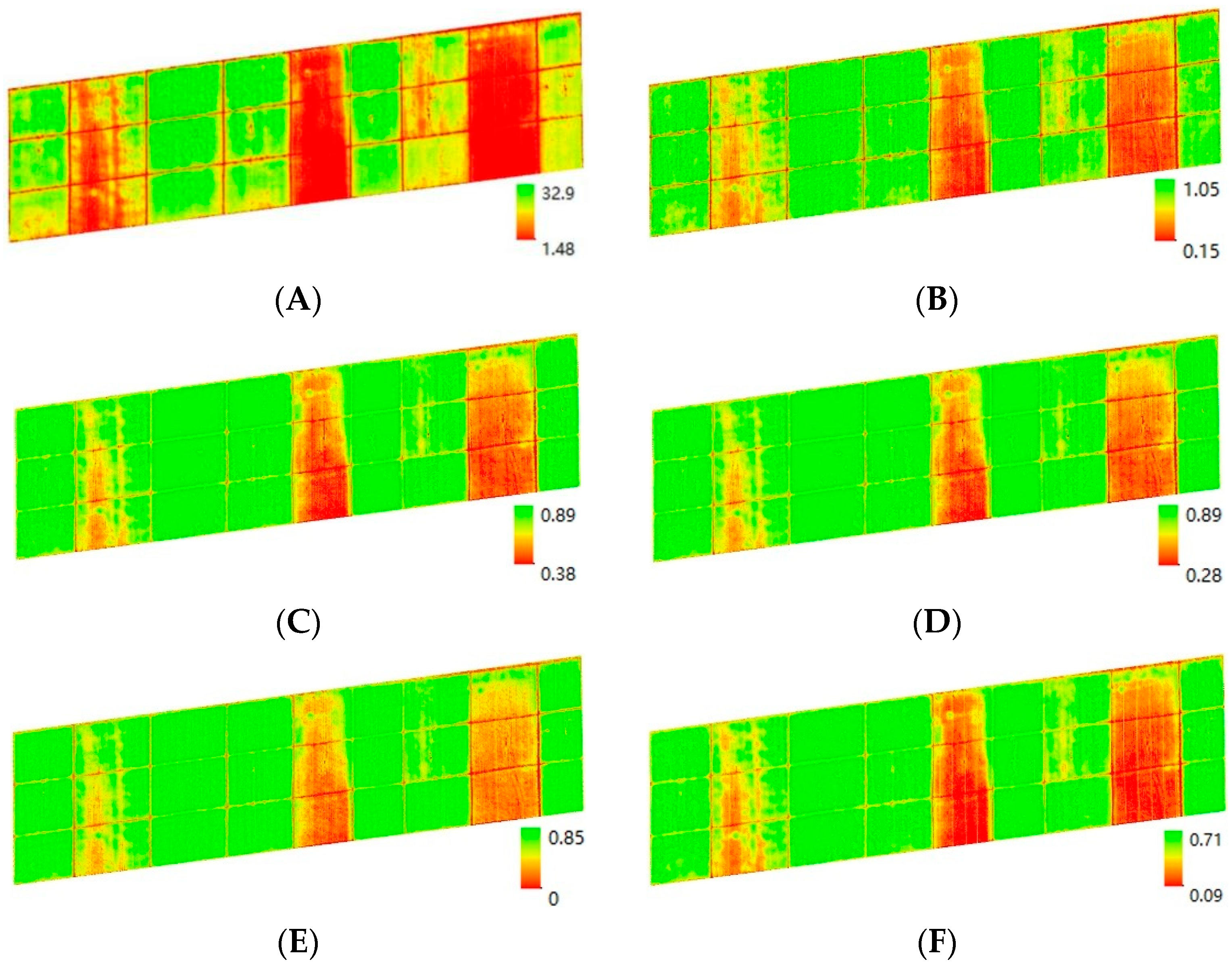
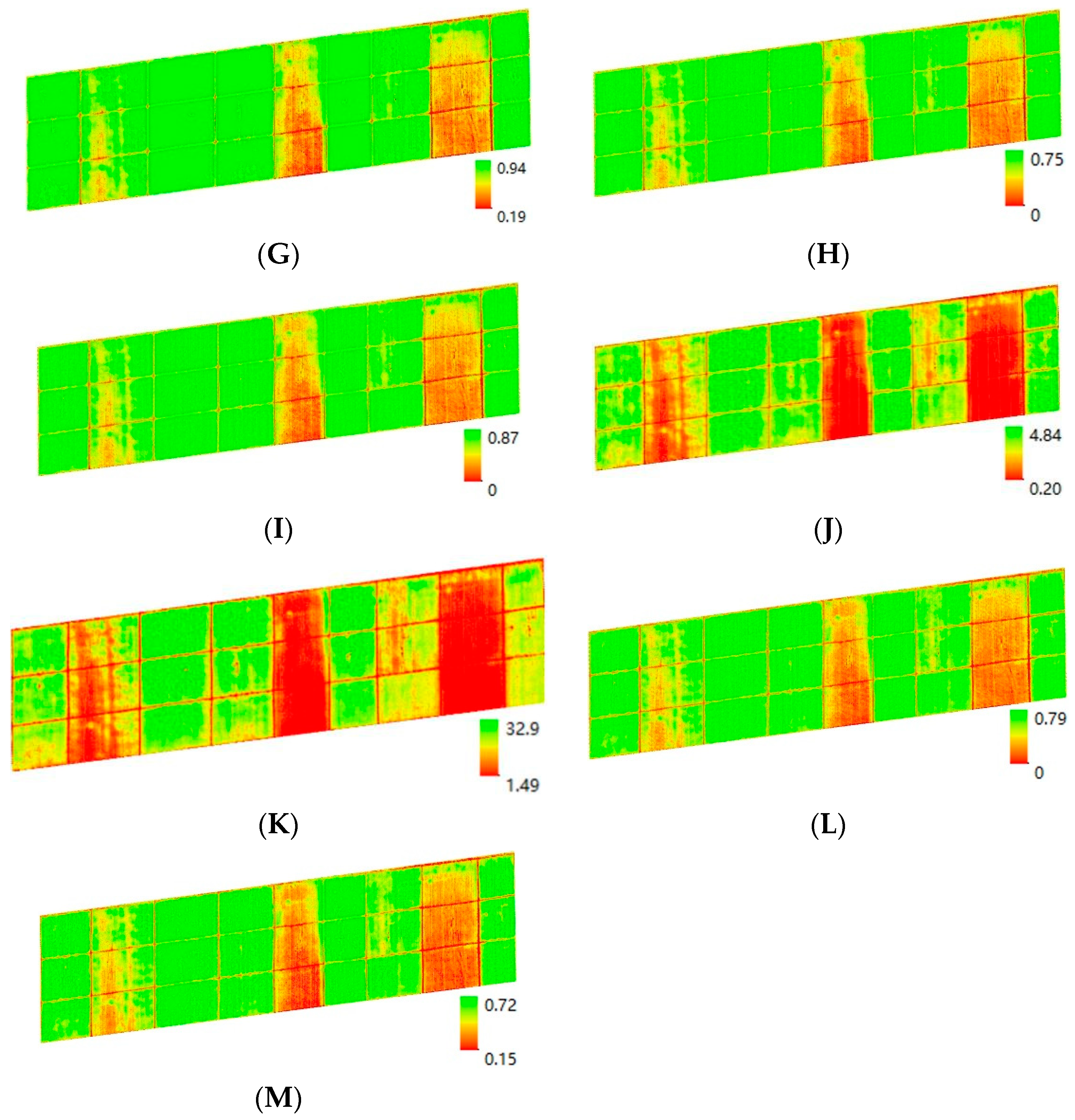
Vegetation index maps not only showed the degree of vegetation vitality but also the water status of wheat plants (Figure 4). In this study, winter wheat was shown to be sensitive to the near-infrared (NIR) and red (R) bands. The reflectance values indicated that wheat plants strongly absorbed red edge wavelength, reflected green band and transmitted near-infrared light more effectively. As a result, the index maps illustrated that vegetation indices such as DVI, RVI, and R-M were effective in reflecting lower vegetation cover and lower CWC with a deeper red color, while vegetation indices such as GNDVI, NDVI, NDRE, OSAVI, and SAVI indicated higher vegetation cover and higher CWC when the near-infrared and green bands were involved in the calculation of vegetation indices. Our findings confirmed that DVI, RVI, and R-M overestimated the drought status, while it could be improved when red edge and green bands were involved in index calculation, such as GNDVI and NDRE.

3.3. Correlation Analysis between Predicted and Observed CWC

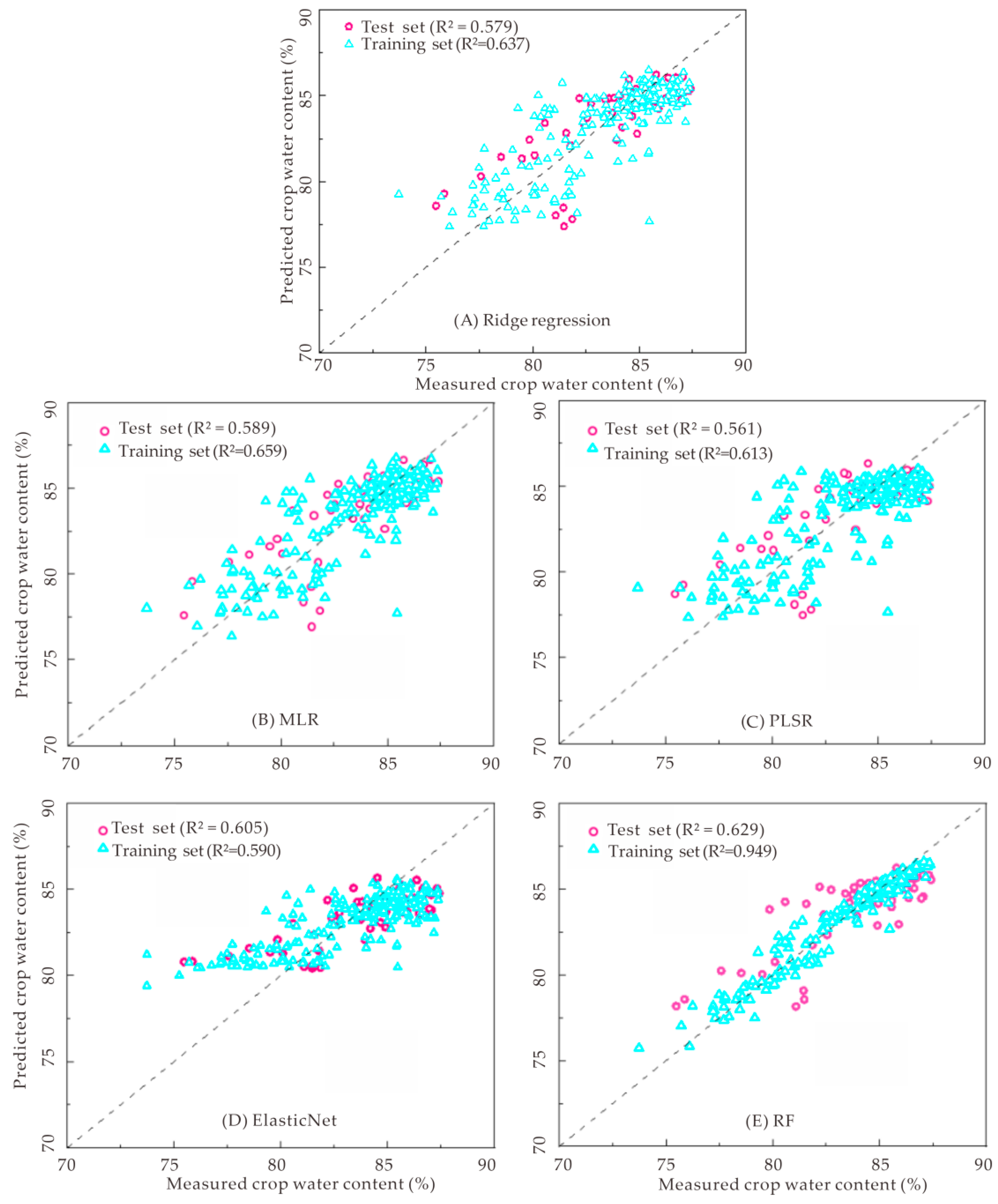
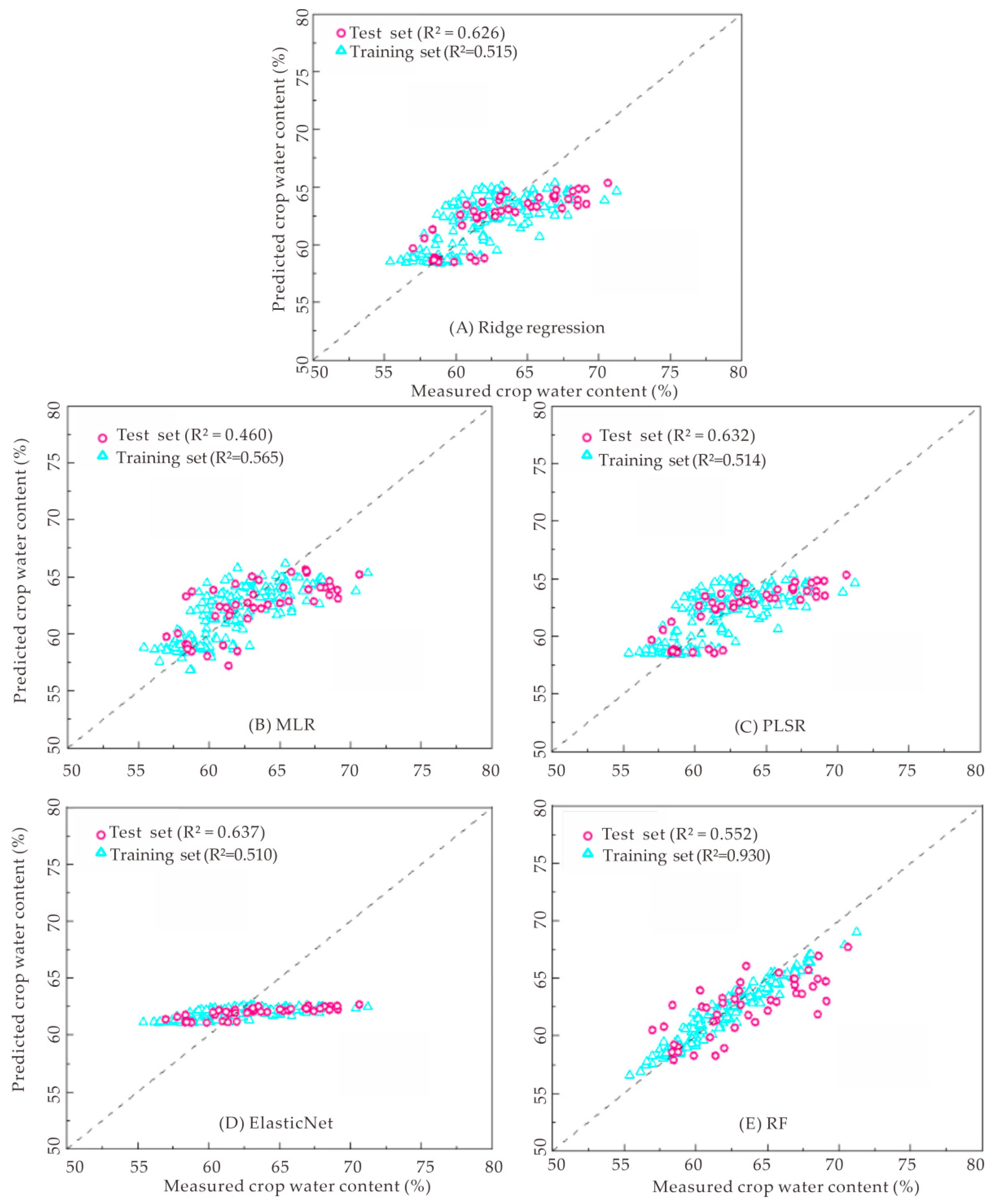
In this study, five machine learning models (MLR, PLSR, ElasticNet, RF, and ridge regression models) were adopted to estimate CWC of winter wheat using thirteen vegetation indices (SAVI, EVI, R-M, NDRE, OSAVI, GOSAVI, REOSAVI, GBNDVI, NDVI, RVI, DVI, GNDVI, and TVI) (Figure 5, Figure 6 and Figure 7). In general, the performance of machine learning models at the jointing and flowering stages was better than that of the grain-filling stage of winter wheat. For example, coefficients of determination (R2) for the training set were 0.590 for ElasticNet, 0.613–0.659 for ridge regression, MLR, and PLSR, and 0.949 for RF, respectively, at the jointing stage. Similarly, R2 values were 0.622 for ElasticNet, 0.643–0.659 for ridge regression, MLR, and PLSR, and 0.943 for RF, respectively, at the flowering stage. The R2 values at the jointing and flowering stages were significantly higher than those of the grain-filling stage, whose R2 values were only 0.510–0.565 for ElasticNet, Ridge regression, MLR, and PLSR, respectively. Overall, the RF model performed best for the training test. For the test set, R2 values were 0.589–0.651 at the jointing stage and 0.769–0.835 at the flowering stage. As for the grain-filling stage, R2 values for the test set significantly decreased, with the values ranging from 0.460 to 0.637. The results indicated that the CWC estimates at the flowering and jointing stages were significantly better than those of the grain-filling stage, and the RF model performed best among all the models.

3.4. Model Evaluation

To assess the performance of the models for estimating CWC, three evaluation metrics were employed, including coefficient of determination (R2), root mean square error (RMSE), and residual prediction deviation (RPD). The random forest (RF) model generated R2 values of 0.930–0.949 for the training set, and 0.552–0.769 for the test set across different growth stages, which were 5.2–56.8% higher than those of the other four models (Table 4). This indicated that RF provided relatively stable accuracy of CWC inversion. Additionally, RF had lower RMSE values (1.323–2.141%) and higher RPD values (2.011–3.820) for training and test sets compared to the other four models. On average, the RMSE values of the RF model were 21.4–50.5% lower and the RPD values of RF were up to 146.3% higher than those of the other four models, demonstrating its superior performance in CWC prediction. Overall, the evaluation indicated that using UAV multispectral remote sensing to monitor CWC was feasible, with the random forest model being the most effective model among those tested.

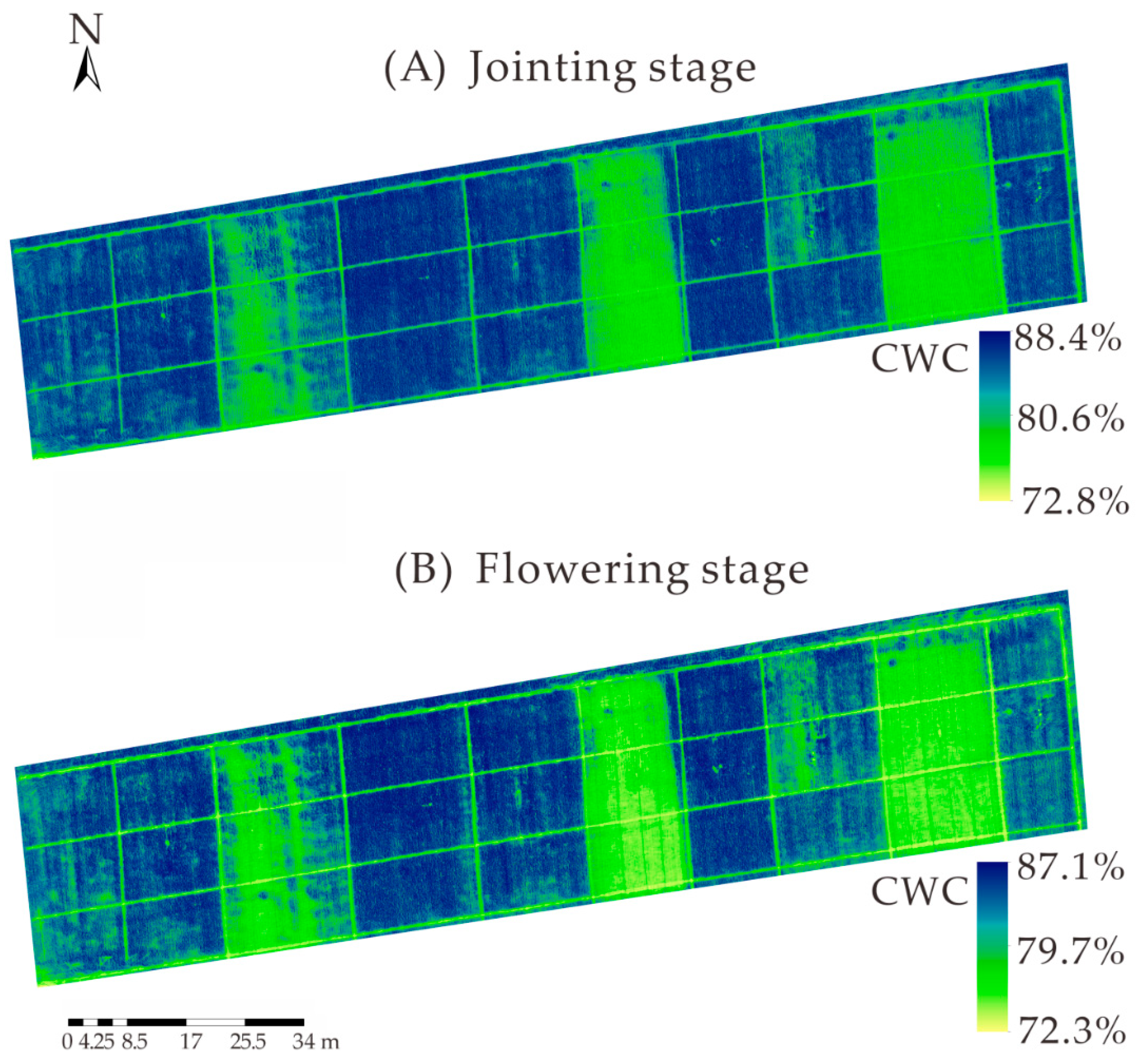
3.5. Construction of CWC Inversion Maps Based on GNDVI and NDRE Using the RF Model

Based on the findings, the green normalized difference vegetation index (GNDVI) and the normalized red edge vegetation index (NDRE) were identified as the best vegetation indices for estimating CWC at the jointing and flowering stages, respectively. Furthermore, the random forest (RF) model was found to be most effective in CWC inversion. Therefore, GNDVI and NDRE were selected to construct accurate CWC inversion maps for winter wheat (Figure 8). The results showed that CWC derived from GNDVI and NDRE was from 72.8% to 88.4% at the jointing stage and from 72.3% to 87.1% at the flowering stage, which was close to the range of measured CWC at the two stages. However, the R2 values were undesirable (0.532–0.599 for training and test sets) at the filling stage. Furthermore, RMSE was relatively higher (2.735% for training and test sets), indicating that the stage might not be a suitable period for CWC inversion using the above mentioned thirteen vegetation indices. GNDVI and NDRE were then found to be the most effective indices for estimating CWC, and the RF model provided the most accurate inversion results at the jointing and flowering stages of winter wheat in the North China Plain.

4. Discussion

4.1. Identification of Optimal Vegetation Indices for CWC Estimation

This study evaluated thirteen vegetation indices—SAVI, EVI, R-M, NDRE, OSAVI, GOSAVI, REOSAVI, GBNDVI, NDVI, RVI, DVI, GNDVI, and TVI—across three growth stages of winter wheat: jointing, flowering, and grain filling. The correlation coefficients between the vegetation indices and crop water content (CWC, %) ranged from 0.64 to 0.82, indicating a barely to preferably acceptable feasibility for using the indices to estimate CWC in winter wheat. At the jointing stage, GNDVI showed the highest correlation, with a coefficient of 0.77, whereas NDRE had the highest correlation at the flowering stage, reaching 0.82. While at the grain-filling stage, R-M and RVI exhibited the highest correlation, both at 0.71. These findings confirm that CWC is more sensitive to near infrared and green bands during the early growth period of winter wheat, while red bands might overestimate the drought status. Similar findings were also observed in the studies by Peng et al. [48], and Liu et al. [49]. Mpho Kapari et al. found that NDRE was the optimal vegetation index variable [50]. Studies have shown that GNDVI is considered to be a reliable indicator for estimating CWC [23]. Our comparative analysis across the growth stages indicated that GNDVI and NDRE were considered as the optimal vegetation indices for estimating CWC at the jointing and flowering stages, respectively. The findings are probably attributable to the fact that GNDVI is effective in reducing the impact of atmospheric and soil background factors [51], improving the accuracy of CWC estimation. Furthermore, NDRE used red edge instead of red band in the index calculation, modifying the excessive inversion of drought, suggesting that red edge was more suitable to inverse CWC status. This finding is also consistent with previous studies indicating that NDRE are highly sensitive to CWC changes of peas and green beans [23]. Previous studies indicated that the selection of vegetation indices with red edge in the middle growth period helped to mitigate the impact of atmospheric, soil, and environmental factors, thereby improving the accuracy of the inversion model [52]. Therefore, in the present study, NDRE had the highest correlation at the flowering stage. This contrasted with the results from Habure et al. [17], who indicated that the SAVI showed good fitting accuracy in leaf moisture estimation. This difference might be attributed to the variations in wheat varieties and climatic zones in a Mediterranean climate, resulting in different reflectance values of crop vegetation [53].

4.2. Identification of Optimal Machine Learning Algorithms for CWC Estimation

The results of this study highlighted several key insights into the effectiveness of machine learning models in predicting CWC using multispectral data. This study compared the accuracy of five machine learning algorithms—MLR, RF, PLSR, ElasticNet, and ridge regression. Numerous experiments and researchers have applied machine learning techniques in CWC predictions [9,11,54], achieving R2 values > 0.75. Different from traditional linear regression, machine learning algorithms were particularly useful in handling complex, large-scale datasets and effectively addressed issues related to overfitting caused by a high number of indices [55].
In this study, the random forest (RF) algorithm provided the best estimation of CWC using multispectral remote sensing data at the flowering stage. The results showed that the random forest R2 reached 0.769 during the flowering period. In addition, RMSE and RPD were 3.002% and 2.011, respectively, which were significantly better than the other four machine learning models. This result is in agreement with the findings by Ndlovu et al. [18], who demonstrated that the RF algorithm is an optimal model for estimating leaf water content at the heading stage of maize. The RF model stood out because it used an ensemble approach based on decision trees [56]. By constructing and combining multiple decision trees, RF enhanced model stability and accuracy. This allowed RF to effectively manage high-dimensional data and capture nonlinear relationships between features, without feature selection or dimensionality reduction [57]. Also, to avoid overfitting of the ML models evaluated in this study, we used a feature selection and structure simplification method to control the complexity of ML models. The outliers in the used dataset were also screened to improve the accuracy of the model and prevent overfitting. In the present study, the reason why the RF model outperformed the other ML models was because the RF model assessed the importance of each feature by building multiple decision trees and randomly selecting features on each tree for segmentation. This helped to identify key spectral features and vegetation indices that are sensitive to CWC [54]. In addition, by integrating the results of multiple decision trees, random forest reduced the possible overfitting risk of a single decision tree, thereby improving the generalization ability of the model, and realizing the accurate monitoring and prediction of CWC of winter wheat plants [56].
In contrast, MLR, PLSR, ElasticNet, and ridge regression were single-model approaches and lacked the benefits of ensemble learning [58]. In this study, MLR showed moderate performance, particularly struggling with high-dimensional data [59]. The challenges associated with high computational complexity and the need for careful preprocessing further impacted the popularization of the MLR model. Up to now, PLSR was mainly designed to handle multicollinearity and high-dimensional data by projecting predictors into a lower-dimensional space [60]. However, it still fell short compared to RF’s ability to manage feature interactions and nonlinearities effectively. As for ElasticNet, this model combined L1 and L2 regularization, offering improved performance over MLR [61]. Nevertheless, the performance of ElasticNet was limited by its inability to fully capture the complex and nonlinear relationships [62]. Ridge regression also showed limitations similar to MLR and ElasticNet. Although it effectively handled multicollinearity and provided stable solutions, its predictive accuracy was lower compared to RF. Besides, it also struggled with capturing the intricate relationships within the multispectral data [63]. The evaluation metrics—R2, RMSE, and RPD—demonstrated that RF not only achieved the highest R2 and RPD values but also the lowest RMSE, indicating the best performance among the models. The RF model’s ability to handle large datasets, its robustness against missing values and outliers, and its high predictive accuracy make the RF model the preferred choice for practical applications in wheat CWC estimation and prediction in the North China Plain. This research primarily relies on the unique climatic conditions and geographical environment of the North China Plain. Due to the variability of weather conditions, experiments may not proceed according to the originally scheduled time, necessitating the collection of experimental data under sunny conditions within the crop’s growing season. During the process of obtaining experimental data, factors such as plants sampling may inadvertently influence the results and CWC measurements.

5. Conclusions

In summary, random forest (RF) was found most effective in estimating crop water content (CWC) from UAV-based multispectral remote sensing data, particularly when combined with the GNDVI and NDRE vegetation indices at the jointing and flowering stages, respectively. The R2 values of the validation set reached 0.629 and 0.769 at the jointing stage and flowering stage, respectively. In addition, the RMSE and RPD of the RF model were 2.035–3.002% and 2.011–2.041 at the jointing and flowering stages, respectively. These values are significantly better than those of other models. Our results confirm that RF-derived estimations can serve as reliable references for field applications in monitoring CWC in winter wheat, enhancing precision in water management practices and contributing to effective irrigation decision making. In conclusion, the inversion method of CWC based on GNDVI and NDRE through the RF model provided valuable insights for practical applications in precision agriculture through advanced remote sensing techniques in the North China Plain. The experimental station is located in the typical South-to-North transition zone of China, which has both the subtropical and temperate climates. This highlights the specific geographical environment and climate factors in the region, and the recommended ML models and vegetation indices may not be universally applicable.
Deploying IoT sensors in farmland and utilizing UAVs for aerial monitoring allow for real-time acquisition of data on soil moisture, crop growth status, and weather conditions. The information is crucial for formulating timely irrigation plans and adjusting water management. By employing variable irrigation systems, based on real-time monitoring of soil moisture and crop water content, appropriate amounts of water can be applied to different plots of the farmland. Additionally, leveraging machine learning algorithms to analyze historical weather data, soil moisture patterns, and crop growth cycles enables the prediction of future water resource demands and the optimization of irrigation strategies, ultimately achieving the goal of rational water resource utilization.
In the future, we will expand the sampling range in the North China Plain by increasing more data samples and introducing more highly correlated and newly established vegetation indices to estimate CWC (Crop Water Content or another relevant abbreviation if specified). Additionally, we will incorporate more machine learning models and deep learning models (Extreme Gradier Boosting Regressor or Histogram Gradier Boosting Regressor) to conduct deeper analysis on the data, aiming to establish a reliable CWC estimation model that is broadly applicable to the North China Plain, thereby creating greater value for the rational utilization of water resources.

Author Contributions

Conceptualization, Z.Z. and A.Q.; methodology, Z.Z.; software, X.Z.; validation, Z.Z. and S.L.; formal analysis, Z.Z.; investigation, Z.Z.; resources, Z.Z. and A.Q.; data curation, Z.Z. and X.Z.; writing—original draft preparation, Z.Z.; writing—review and editing, A.Q. and Y.G.; visualization, A.Q.; supervision, A.Q.; project administration, G.D. and Y.G.; funding acquisition, G.D. and Y.G. All authors have read and agreed to the published version of the manuscript.

Funding

This research was funded by the Henan Provincial Key Science and Technology Project (221100110700), the Major Science and Technology Project of Shandong Province (2023TZXD011), the National Key Research and Development Program of China (2023YFD1900802), and “The APC was funded by the Henan Provincial Key Science and Technology Project”.

Data Availability Statement

The data are available upon reasonable request to the corresponding authors.

Acknowledgments

The authors thank the reviewers’ and editor’s comments on improving the quality of the manuscript.

Conflicts of Interest

The authors declare no conflicts of interest.

References

  1. Yuan, G.F.; Tang, D.Y.; Luo, Y.; Yu, Q. Advances in Crop Water Stress Research Based on Canopy Temperature. Adv. Earth Sci. 2001, 16, 45–54, (In Chinese with English Abstract). [Google Scholar]
  2. Xue, L.H.; Cao, W.X.; Tian, Y.C. Advances in Spectral Diagnosis of Crop Water and Nitrogen Status. J. Remote Sens. 2003, 7, 73–80. [Google Scholar]
  3. Cheng, T.; Rivard, B.; Sanchez-Azofeifa, A.G.; Féret, J.-B.; Jacquemoud, S.; Ustin, S.L. Predicting Leaf Gravimetric Water Content from Foliar Reflectance across a Range of Plant Species Using Continuous Wavelet Analysis. J. Plant Physiol. 2012, 169, 1134–1142. [Google Scholar] [CrossRef] [PubMed]
  4. Yu, J.; Zhang, S.; Zhang, Y.; Hu, R.; Lawi, A.S. Construction of a Winter Wheat Comprehensive Growth Monitoring Index Based on a Fuzzy Degree Comprehensive Evaluation Model of Multispectral UAV Data. Sensors 2023, 23, 8089. [Google Scholar] [CrossRef]
  5. Feng, H.; Tao, H.; Li, Z.; Yang, G.; Zhao, C. Comparison of UAV RGB Imagery and Hyperspectral Remote-Sensing Data for Monitoring Winter Wheat Growth. Remote Sens. 2022, 14, 3811. [Google Scholar] [CrossRef]
  6. Pei, H.; Feng, H.; Li, C.; Jin, X.; Li, Z.; Yang, G. Remote Sensing Monitoring of Winter Wheat Growth with UAV Based on Comprehensive Index. Trans. Chin. Soc. Agric. Engin. 2017, 33, 74–82, (In Chinese with English Abstract). [Google Scholar]
  7. Wen, S.; Liu, Z.; Han, Y.; Chen, Y.; Xu, L.; Li, Q. Spatiotemporal Variation Characteristics of Reference Evapotranspiration and Relative Moisture Index in Heilongjiang Investigated through Remote Sensing Tools. Remote Sens. 2023, 15, 2582. [Google Scholar] [CrossRef]
  8. Zheng, W.; Zhang, J.; He, Y.; Liu, H.; Chen, M. A Review of Vegetation Indices and Their Application in Remote Sensing of Crop Water Content. Agric. Water Manag. 2023, 279, 107903. [Google Scholar] [CrossRef]
  9. Cassanelli, D.; Lenzini, N.; Ferrari, L.; Rovati, L. Partial Least Squares Estimation of Crop Moisture and Density by Near-Infrared Spectroscopy. IEEE Trans. Instrum. Meas. 2021, 70, 1004510. [Google Scholar] [CrossRef]
  10. Li, C.; Wang, Y.C.; Li, X.Q.; Yang, X.F.; Gu, X.H. Estimation Model of Wheat Plant Component Moisture Content Based on Wavelet Technology. J. Agric. Mach. 2021, 52, 193–201. [Google Scholar] [CrossRef]
  11. Torres-Tello, J.W.; Ko, S. A Novel Approach to Identify the Spectral Bands That Predict Moisture Content in Canola and Wheat. Biosyst. Eng. 2021, 210, 91–103. [Google Scholar] [CrossRef]
  12. Han, G. Research on Wheat Plant Water Status Monitoring Based on Hyperspectral Data. Ph.D. Thesis, Northwest A&F University, Yangling, China, 2011. [Google Scholar]
  13. Wang, Q.; Yi, Q.X.; Bao, A.M.; Zhao, J. Study on Hyperspectral Indices for Estimating Cotton Canopy Water Content. Spectrosc. Spect. Anal. 2013, 33, 507–512. [Google Scholar] [CrossRef]
  14. Jiang, J.; Liu, D.; Zheng, Z.; Shi, Y.; Wang, L. Evaluating the Performance of Machine Learning Models for Predicting Crop Water Stress Using Sentinel-2 Data. Agric. Water Manag. 2023, 274, 107964. [Google Scholar] [CrossRef]
  15. Yang, C.; Cheng, J.; Liu, B.; Zhang, W.; Huang, J. Assessment of the Potential of Machine Learning Approaches for Estimating Crop Water Status Using Multi-Source Remote Sensing Data. Remote Sens. Appl. Soc. Environ. 2024, 29, 100581, (In Chinese with English Abstract). [Google Scholar]
  16. Zhang, Y.W.; Wang, S.M.; Chen, D.; Wang, Y.; Fu, H. Detection Methods of Wheat Plant Water Content Based on Near-Infrared Reflectance. J. Agric. Mach. 2017, 48 (Suppl. S1), 118–122+261, (In Chinese with English Abstract). [Google Scholar]
  17. Habure, T.; Zhang, B.Z.; Li, S.E.; Peng, Z.G.; Han, N.N.; Liu, L.L. Diagnosis of Winter Wheat Plant Water Content Based on Canopy Spectral Characteristics. Irrig. Drain. 2018, 37, 9–15, (In Chinese with English Abstract). [Google Scholar]
  18. Ndlovu, H.S.; Odindi, J.; Sibanda, M.; Mutanga, O.; Clulow, A.; Chimonyo, V.G.P.; Mabhaudhi, T. A Comparative Estimation of Maize Leaf Water Content Using Machine Learning Techniques and Unmanned Aerial Vehicle (UAV)-Based Proximal and Remotely Sensed Data. Remote Sens. 2021, 13, 4091. [Google Scholar] [CrossRef]
  19. Han, D.; Liu, S.; Du, Y.; Xie, X.; Fan, L.; Lei, L.; Li, Z.; Yang, H.; Yang, G. Crop Water Content of Winter Wheat Revealed with Sentinel-1 and Sentinel-2 Imagery. Sensors 2019, 19, 4013. [Google Scholar] [CrossRef]
  20. Hassan-Esfahani, L.; Torres-Rua, A.; Jensen, A.; McKee, M. Assessment of Surface Soil Moisture Using High-Resolution Multi-Spectral Imagery and Artificial Neural Networks. Remote Sens. 2015, 7, 2627–2646. [Google Scholar] [CrossRef]
  21. Chen, S.B.; Chen, J.Y.; Zhang, Z.T.; Bian, J.; Wang, Y.F.; Shi, S.L. Estimation of Soil Moisture Content in Winter Wheat at the Booting Stage Using UAV Multispectral Remote Sensing. Water Saving Irrig. 2018, 22, 39–43, (In Chinese with English Abstract). [Google Scholar]
  22. Chen, J.Y.; Chen, S.B.; Zhang, Z.T.; Fu, Q.P.; Bian, J.; Cui, T. Estimation of Cotton Photosynthetic Parameters at the Budding Stage Using UAV Multispectral Remote Sensing. J. Agric. Mach. 2018, 49, 230–239. [Google Scholar] [CrossRef]
  23. Mndela, Y.; Ndou, N.; Nyamugama, A. Irrigation Scheduling for Small-Scale Crops Based on Crop Water Content Patterns Derived from UAV Multispectral Imagery. Sustainability 2023, 15, 12034. [Google Scholar] [CrossRef]
  24. Wang, X.; Wang, Z.; Xu, L.; Liu, H.; Zhang, L. Evaluation of Vegetation Indices for Monitoring Crop Water Stress in the North China Plain. Field Crops Res. 2024, 287, 108847. [Google Scholar] [CrossRef]
  25. Huete, A.R. A Soil-Adjusted Vegetation Index (SAVI). Remote Sens. Environ. 1988, 25, 295–309. [Google Scholar] [CrossRef]
  26. Wang, Z.; Liu, C.; Huete, A.R. Advances in Vegetation Index Research from AVHRR-NDVI to MODIS-EVI. Acta Ecol. Sin. 2003, 23, 1649–1661. [Google Scholar]
  27. Gitelson, A.A.; Gritz, Y.; Merzlyak, M.N. Relationships Between Leaf Chlorophyll Content and Spectral Reflectance and Algorithms for Non-Destructive Chlorophyll Assessment in Higher Plant plant. J. Plant Physiol. 2003, 160, 271–282. [Google Scholar] [CrossRef]
  28. Barnes, E.M.; Clarke, T.; Richards, S.E.; Colaizzi, P.D.; Haberland, J.; Kostrzewski, M.; Waller, P.; Choi, C.; Riley, E.; Thompson, T.; et al. Coincident Detection of Crop Water Stress, Nitrogen Status, and Canopy Density Using Ground-Based Multispectral Data. In Proceedings of the 4th International Conference on Precision Agriculture, Minneapolis, MN, USA, 16–19 July 2000. [Google Scholar]
  29. Cao, Q.; Miao, Y.; Shen, J.; Yu, W.; Yuan, F.; Cheng, S.; Huang, S.; Wang, H.; Yang, W.; Liu, F. Improving In-Season Estimation of Rice Yield Potential and Responsiveness to Topdressing Nitrogen Application with Crop Circle Active Crop Canopy Sensor. Precis. Agric. 2015, 17, 136–154. [Google Scholar] [CrossRef]
  30. Gilabert, M.A.; González-Piqueras, J.; García-Haro, F.J.; Meliá, J. A Generalized Soil-Adjusted Vegetation Index. Remote Sens. Environ. 2002, 82, 303–310. [Google Scholar] [CrossRef]
  31. Lu, J.; Miao, Y.; Shi, W.; Li, J.; Yuan, F. Evaluating Different Approaches to Non-Destructive Nitrogen Status Diagnosis of Rice Using Portable RapidSCAN Active Canopy Sensor. Sci. Rep. 2017, 7, 14073. [Google Scholar] [CrossRef]
  32. Gitelson, A.A.; Kaufman, Y.J.; Merzlyak, M.N. Use of a Green Channel in Remote Sensing of Global Vegetation from EOS-MODIS. Remote Sens. Environ. 1996, 58, 289–298. [Google Scholar] [CrossRef]
  33. Rouse, J.W.; Haas, R.H.; Deering, D.W.; Schell, J.A.; Harlan, J.C. Monitoring the Vernal Advancement and Retrogradation (Green Wave Effect) of Natural Vegetation. In Proceedings of the Third Earth Resources Technology Satellite-1 (ERTS-1) Symposium, Washington, DC, USA, 10–14 December 1973. [Google Scholar]
  34. Schuerger, A.C.; Capelle, G.A.; Di Benedetto, J.A.; Mao, C.; Thai, C.N.; Evans, M.D.; Richards, J.T.; A Blank, T.; Stryjewski, E.C. Comparison of Two Hyperspectral Imaging and Two Laser-Induced Fluorescence Instruments for the Detection of Zinc Stress and Chlorophyll Concentration in Bahia Grass (Paspalum notatum Flugge). Remote Sens. Environ. 2003, 84, 572–588. [Google Scholar] [CrossRef]
  35. Jordan, C.F. Derivation of Leaf-Area Index from Quality of Light on the Forest Floor. Ecology 1969, 50, 663–666. [Google Scholar] [CrossRef]
  36. Deering, D.W.; Rouse, J.W.; Haas, R.H.; Schell, J.A. Measuring “Forage Production” of Grazing Units from Landsat MSS Data. In Proceedings of the Second Earth Resources Technology Satellite-1 (ERTS-1) Symposium, Washington, DC, USA, 6 October 1975. [Google Scholar]
  37. Guo, X.; Liu, X.; Song, G. Multiple Linear Regression Analysis. In Textbook of Medical Statistics.; Guo, X., Xue, F., Eds.; Springer: Singapore, 2024. [Google Scholar] [CrossRef]
  38. Chakraborty, A.; Goswami, D. Prediction of slope stability using multiple linear regression (MLR) and artificial neural network (ANN). Arab. J. Geosci. 2017, 10, 385. [Google Scholar] [CrossRef]
  39. Elsherbiny, O.; Fan, Y.; Zhou, L.; Qiu, Z. Fusion of Feature Selection Methods and Regression Algorithms for Predicting the Canopy water Content of Rice Based on Hyperspectral Data. Agriculture 2021, 11, 51. [Google Scholar] [CrossRef]
  40. Zhang, Y.; Liu, J.; Shen, W. A Review of Ensemble Learning Algorithms Used in Remote Sensing Applications. Appl. Sci. 2022, 12, 8654. [Google Scholar] [CrossRef]
  41. Chan, J.Y.L.; Leow, S.M.H.; Bea, K.T.; Cheng, W.K.; Phoong, S.W.; Hong, Z.W.; Chen, Y.L. Mitigating the Multicollinearity Problem and Its Machine Learning Approach: A Review. Mathematics 2022, 10, 1283. [Google Scholar] [CrossRef]
  42. Muthukrishnan, R.; Rohini, R. LASSO: A feature selection technique in predictive modeling for machine learning. In Proceedings of the 2016 IEEE International Conference on Advances in Computer Applications (ICACA), Coimbatore, India, 24 October 2016; pp. 18–20. [Google Scholar] [CrossRef]
  43. Rauschenberger, A.; Glaab, E.; van de Wiel, M.A. Predictive and interpretable models via the stacked elastic net. Bioinformatics 2021, 37, 2012–2016. [Google Scholar] [CrossRef]
  44. Srivatsaan, S.; Sankar, A.; Karthikeyan, M. Impact of elastic net and LASSO regularization techniques on the NHANES dataset. AIP Conf. Proc. 2024, 3075, 020208. [Google Scholar] [CrossRef]
  45. Boulesteix, A. PLS Dimension Reduction for Classification with Microarray Data. Stat. Appl. Genet. Mol. 2004, 3, 33. [Google Scholar] [CrossRef]
  46. Kvalheim, O.M.; Arneberg, R.; Bleie, O.; Rajalahti, T.; Smilde, A.K.; Westerhuis, J.A. Variable importance in latent variable regression models. J. Chemom. 2014, 28, 615–622. [Google Scholar] [CrossRef]
  47. Askari, M.S.; O’Rourke, S.M.; Holden, N.M. Evaluation of soil quality for agricultural production using visible–near-infrared spectroscopy. Geoderma 2015, 243, 80–91. [Google Scholar] [CrossRef]
  48. Peng, Z.; Lin, S.; Zhang, B.; Wei, Z.; Liu, L.; Han, N.; Cai, J.; Chen, H. Winter wheat canopy water content monitoring based on spectral transforms and “three-edge” parameters. Agric. Water Manag. 2020, 240, 106306. [Google Scholar] [CrossRef]
  49. Liu, L.; Wang, J.; Huang, W.; Zhao, C.; Zhang, B.; Tong, Q. Estimating winter wheat plant water content using red edge parameters. Int. J. Remote Sens. 2004, 25, 3331–3342. [Google Scholar] [CrossRef]
  50. Kapari, M.; Sibanda, M.; Magidi, J.; Mabhaudhi, T.; Nhamo, L.; Mpandeli, S. Comparing Machine Learning Algorithms for Estimating the Maize Crop Water Stress Index (CWSI) Using UAV-Acquired Remotely Sensed Data in Smallholder Croplands. Drones 2024, 8, 61. [Google Scholar] [CrossRef]
  51. Yin, C.; Wang, Z.; Lv, X.; Qin, S.; Ma, L.; Zhang, Z.; Tang, Q. Reducing soil and leaf shadow interference in UAV imagery for cotton nitrogen monitoring. Front. Plant Sci. 2024, 15, 1380306. [Google Scholar] [CrossRef]
  52. Dong, T.; Liu, J.; Shang, J.; Qian, B.; Ma, B.; Kovacs, J.M.; Walters, D.; Jiao, X.; Geng, X.; Shi, Y. Assessment of red-edge vegetation indices for crop leaf area index estimation. Remote Sens. Environ. 2019, 222, 133–143. [Google Scholar] [CrossRef]
  53. Kyratzis, A.C.; Skarlatos, D.P.; Menexes, G.C.; Vamvakousis, V.F.; Katsiotis, A. Assessment of vegetation indices derived by UAV imagery for durum wheat phenotyping under a water limited and heat stressed Mediterranean environment. Front. Plant Sci. 2017, 8, 1114. [Google Scholar] [CrossRef]
  54. Xu, Q.; Hu, Z.; Chen, Z.; Li, Q.; Zhao, Y. Application of Random Forest and Support Vector Machine for Estimating Crop Water Content Using High-Resolution Remote Sensing Data. Comput. Electron. Agric. 2024, 194, 106748. [Google Scholar] [CrossRef]
  55. Al-Jarrah, O.Y.; Yoo, P.D.; Muhaidat, S.; Karagiannidis, G.K.; Taha, K. Efficient machine learning for big data: A review. Big Data Res. 2015, 2, 87–93. [Google Scholar] [CrossRef]
  56. Ahmad, M.W.; Reynolds, J.; Rezgui, Y. Predictive modelling for solar thermal energy systems: A comparison of support vector regression, random forest, extra trees and regression trees. J. Clean. Prod. 2018, 203, 810–821. [Google Scholar] [CrossRef]
  57. Zebari, R.; Abdulazeez, A.; Zeebaree, D.; Zebari, D.; Saeed, J. A comprehensive review of dimensionality reduction techniques for feature selection and feature extraction. J. Appl. Sci. Technol. Trends 2020, 1, 56–70. [Google Scholar] [CrossRef]
  58. Hu, T.; Zhang, X.; Bohrer, G.; Liu, Y.; Zhou, Y.; Martin, J.; Li, Y.; Zhao, K. Crop yield prediction via explainable AI and interpretable machine learning: Dangers of black box models for evaluating climate change impacts on crop yield. Agr. Forest Meteorol. 2023, 336, 109458. [Google Scholar] [CrossRef]
  59. Hussain, J.N. High dimensional data challenges in estimating multiple linear regression. J. Phys. Conf. Series. 2020, 1591, 012035, (IOP Publishing). [Google Scholar] [CrossRef]
  60. Alsouki, L. Functional data regression with prediction and interpretability: Property inference in chemometrics with sparse Partial Least Squares (PLS). Ph.D. Thesis, Université Claude Bernard-Lyon I, Lyon, France, Université Saint-Joseph (Beyrouth), Beirut, Lebanon, 2023. [Google Scholar]
  61. Guo, L. Extreme Learning Machine with Elastic Net Regularization. Intell. Autom. Soft Comput. 2020, 26, 421–427. [Google Scholar] [CrossRef]
  62. Tay, J.K. Extending the Reach of the Lasso and Elastic Net Penalties: Methodology and Practice. Ph.D. Thesis, Stanford University, Stanford, CA, USA, 2021. [Google Scholar]
  63. Fei, S.; Hassan, M.A.; He, Z.; Chen, Z.; Shu, M.; Wang, J.; Li, C.; Xiao, Y. Assessment of Ensemble Learning to Predict Wheat Grain Yield Based on UAV-Multispectral Reflectance. Remote Sens. 2021, 13, 2338. [Google Scholar] [CrossRef]
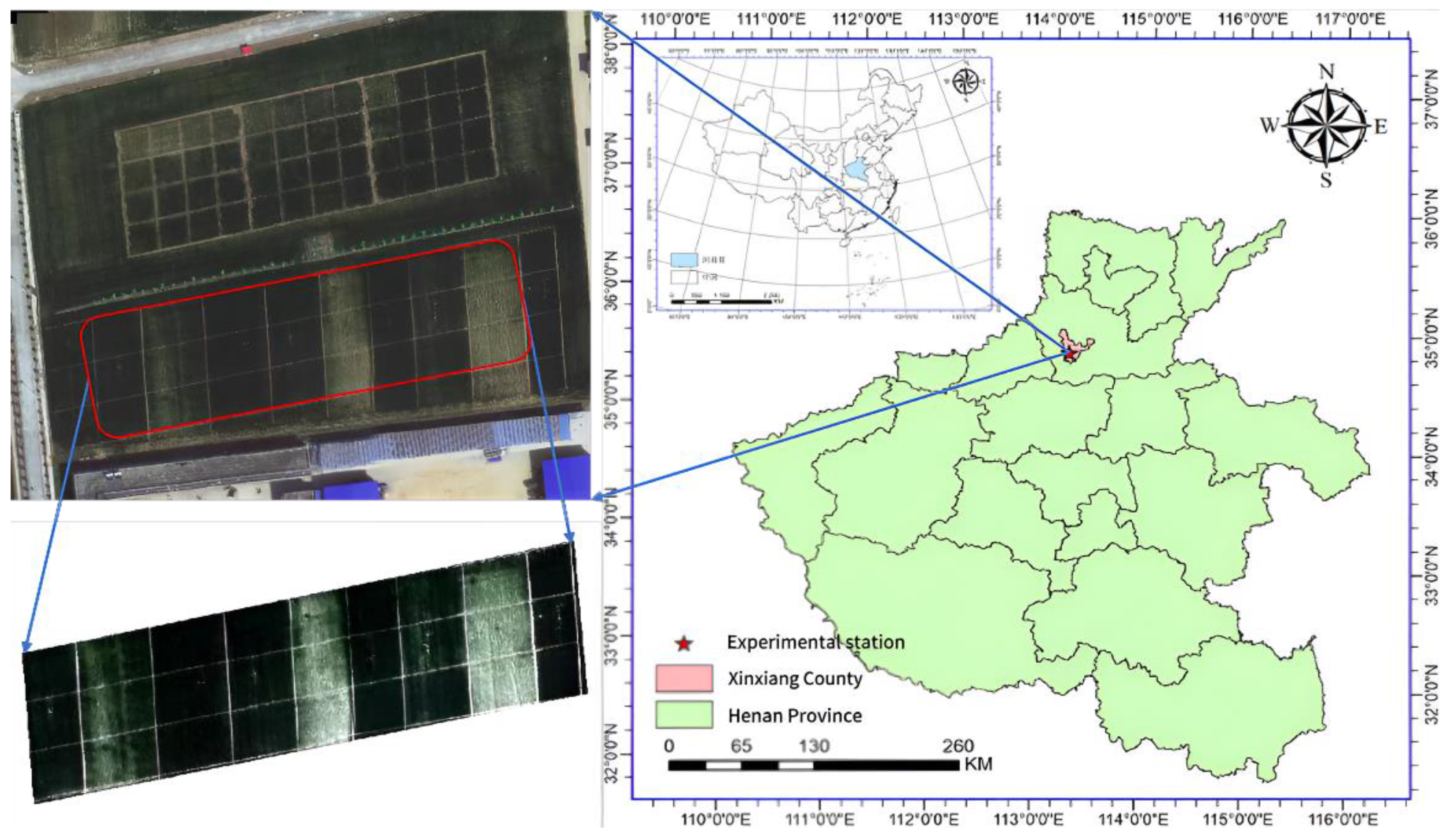
Figure 1. The schematic map of the experimental station and the experimental plots at the station.
Agronomy 14 02361 g001
Figure 2. The specific flowchart of data analysis and processing using different vegetation indices and machine learning algorithms.
Agronomy 14 02361 g002
Figure 3. Correlation analysis between crop water content (%) and vegetation indices at (A) jointing, (B) flowering, and (C) filling stages of winter wheat in 2024.
Agronomy 14 02361 g003
Figure 4. Vegetation index maps of (A) DVI, (B) EVI, (C) GBNDVI, (D) GNDVI, (E) GOSAVI, (F) NDRE, (G) NDVI, (H) OSAVI, (I) REOSAVI, (J) R-M, (K) RVI, (L) SAVI, and (M) TVI at the flowering stage of winter wheat in 2024.
Agronomy 14 02361 g004aAgronomy 14 02361 g004b
Figure 5. Correlation analysis between measured crop water content (CWC, %) and predicted CWC based on (A) ridge regression, (B) multiple linear regression (MLR), (C) partial least squares regression (PLSR), (D) ElasticNet regression, and (E) random forest (RF) models at the jointing stage of winter wheat in 2024. The dashed lines are 1:1 lines.
Agronomy 14 02361 g005
Figure 6. Correlation analysis between measured crop water content (CWC, %) and predicted CWC based on (A) ridge regression, (B) multiple linear regression (MLR), (C) partial least squares regression (PLSR), (D) ElasticNet regression, and (E) random forest (RF) models at the flowering stage of winter wheat in 2024. The dashed lines are 1:1 lines.
Agronomy 14 02361 g006
Figure 7. Correlation analysis between measured crop water content (CWC, %) and predicted CWC based on (A) ridge regression, (B) multiple linear regression (MLR), (C) partial least squares regression (PLSR), (D) ElasticNet regression, and (E) random forest (RF) models at the filling stage of winter wheat in 2024. The dashed lines are 1:1 lines.
Agronomy 14 02361 g007
Figure 8. Inversion maps of crop water content in winter wheat at (A) the jointing stage based on GNDVI, and (B) the flowering stage based on NDRE using RF model.
Agronomy 14 02361 g008
Table 1. Soil physical properties in the experimental area measured at the beginning of the experiment in October 2023.
Soil Depth (cm)Clay (%)Silt (%)Sand (%)Wilt Point
(cm3 cm−3)
Field Capacity (cm3 cm−3)SSWC 1
(cm3 cm−3)
Bulk Density
(g cm−3)
0–206.7569.7223.530.160.340.451.52
20–406.4166.9426.690.160.320.411.51
40–6010.1969.6219.850.180.320.421.52
60–8010.1673.4416.410.180.300.361.42
80–1008.2275.7416.020.170.310.381.41
1 SSWC: Saturated soil water content.
Table 2. Specifications of multispectral camera used in the present experiment.
BandBandwidthWavelengthPicture Resolution
Blue30 nm4501280 × 960
Green30 nm5551280 × 960
Red30 nm6601280 × 960
Red Edge 0120 nm7201280 × 960
Red Edge 0220 nm7501280 × 960
Near infrared30 nm8401280 × 960
Table 3. Vegetation index and calculating formula adopted in the experiment.
Vegetation IndexFormulaReferences
Soil-adjusted vegetation index (SAVI)(1 + 0.5) × (NIR − R)/(NIR + R + 0.5)[25]
Enhanced vegetation index (EVI)2.5 × (NIR − R)/(NIR + 6R − 7.5B + 1)[26]
Red edge model (R-M)NIR/(RE − 1)[27]
Normalized red edge vegetation index (NDRE)(NIR − RE)/(NIR + RE)[28]
Optimized soil-adjusted vegetation index (OSAVI)(NIR − R)/(NIR + R + 0.16)[29]
Green optimized soil-adjusted vegetation index (GOSAVI)(NIR − R)/(NIR + G + 0.16)[30]
Red edge optimized soil-adjusted vegetation index (REOSAVI)(NIR − R)/(NIR + R + 0.16)[31]
Normalized blue-green band difference vegetation index (GBNDVI)(NIR − G + B)/(NIR + G + B)[32]
Normalized difference vegetation index (NDVI)(NIR − R)/(NIR + R)[33]
Ratio vegetation index (RVI)NIR/R[34]
Difference vegetation index (DVI)NIR − R[35]
Green normalized difference vegetation index (GNDVI)(NIR − G)/(NIR + G)[32]
Triangular vegetation index (TVI)1.5 × (NIR − R)/(NIR + RE + 0.5)[36]
Table 4. Evaluation metrics assessing the accuracy of machine learning models for crop water content (%) prediction in the North China Plain, 2024.
Growth StagesModelsTraining SetTest Set
R2RMSE (%)RPDR2RMSE (%)RPD
JointingMLR0.6592.5271.7210.5892.8211.578
RF0.9491.1414.1220.6292.0352.041
ElasticNet0.6132.2581.4050.5612.4241.474
Ridge0.6372.7611.6610.5792.6521.553
PLSR0.6132.8381.6250.5612.9621.524
FloweringMLR0.6592.3741.5210.823.7101.003
RF0.9431.2563.4030.7693.0022.011
ElasticNet0.6223.8711.1210.8304.2071.038
Ridge0.6472.9241.4440.8443.6841.446
PLSR0.6432.5961.4410.8353.9381.442
FillingMLR0.5652.5831.7130.4601.1492.367
RF0.9301.5743.9350.5521.2862.083
ElasticNet0.5102.3511.5740.6371.4762.145
Ridge0.5152.8621.6950.6261.9422.544
PLSR0.5142.1781.6890.6321.7292.472
Note: R2, coefficient of determination; RMSE, root mean square error; and RPD, relative prediction deviation.
Disclaimer/Publisher’s Note: The statements, opinions and data contained in all publications are solely those of the individual author(s) and contributor(s) and not of MDPI and/or the editor(s). MDPI and/or the editor(s) disclaim responsibility for any injury to people or property resulting from any ideas, methods, instructions or products referred to in the content.