Prediction of Anthocyanin Content in Purple-Leaf Lettuce Based on Spectral Features and Optimized Extreme Learning Machine Algorithm

Abstract

Monitoring anthocyanins is essential for assessing nutritional value and the growth status of plants. This study aimed to utilize hyperspectral technology to non-destructively monitor anthocyanin levels. Spectral data were preprocessed using standard normal variate (SNV) and first-derivative (FD) spectral processing. Feature wavelengths were selected using uninformative variable elimination (UVE) and UVE combined with competitive adaptive reweighted sampling (UVE + CARS). The optimal two-band vegetation index (VI2) and three-band vegetation index (VI3) were then calculated. Finally, dung beetle optimization (DBO), subtraction-average-based optimization (SABO), and the whale optimization algorithm (WOA) optimized the extreme learning machine (ELM) for modeling. The results indicated the following: (1) For the feature band selection methods, the UVE-CARS-SNV-DBO-ELM model achieved an R_m² of 0.8623, an RMSE_m of 0.0098, an R_v² of 0.8617, and an RMSE_v of 0.0095, resulting in an RPD of 2.7192, further demonstrating that UVE-CARS enhances feature band extraction based on UVE and indicating a strong model performance. (2) For the vegetation index, VI3 showed a better predictive accuracy than VI2. The VI3-WOA-ELM model achieved an R_m² of 0.8348, an RMSE_m of 0.0109 mg/g, an R_v² of 0.812, an RMSE_v of 0.011 mg/g, and an RPD of 2.3323, demonstrating good performance. (3) For the optimization algorithms, the DBO, SABO, and WOA all performed well in optimizing the ELM model. The R² of the DBO model increased by 5.8% to 27.82%, that of the SABO model by 2.92% to 26.84%, and that of the WOA model by 3.75% to 27.51%. These findings offer valuable insights for future anthocyanin monitoring using hyperspectral technology, highlighting the effectiveness of feature selection and optimization algorithms for accurate detection.

1. Introduction

In recent years, based on epidemiological studies, there has been an increasing awareness of the health benefits of phytochemicals [1,2]. Anthocyanins are the most prominent class of flavonoids and serve as important pigments in plants, responsible for the vibrant purple, pink, red, and blue hues observed in various plant species [3]. Anthocyanins help eliminate free radicals and protect cells from oxidative damage, thereby contributing to the prevention of chronic diseases and the promotion of health [4]. In addition, anthocyanins enhance plant resistance, helping plants withstand various biotic and abiotic stresses [5]. Anthocyanins can absorb excess visible light and help plants resist ultraviolet rays, enhancing their antioxidant properties and acting as natural photoprotectants to prevent light damage [6]. A decrease in anthocyanin levels can lead to impaired photosynthesis and reduced antioxidant capacity in winter wheat, weakening its stress resistance and limiting growth and development [7]. Thus, anthocyanins play a crucial role in regulating the photosynthetic performance of plants. The timely monitoring of anthocyanin content is essential for assessing nutritional value and understanding plant growth conditions. While existing methods for measuring anthocyanin content, such as high-performance liquid chromatography (HPLC) [8] and spectrophotometry [9], provide valuable data, they are hindered by challenges such as high resource consumption, potential damage to plant tissues, and the inability to enable rapid, large-scale, real-time monitoring. Therefore, there is an urgent need to develop an accurate and efficient technique for predicting anthocyanin content. Hyperspectral technology, known for its high spectral resolution and ability to nondestructively detect the internal chemical components of plants, has emerged as a powerful tool in physiological and agricultural research [10,11,12]. Hyperspectral data can reflect the physiological and biochemical characteristics of plants, such as their nitrogen content [13], phosphorus content [14], and chlorophyll content [11], and assist in nutrient prediction [15]. They have also been shown to have potential in assessing pigment levels in plants [16,17]. This capability makes hyperspectral imaging a valuable tool for understanding plant health and optimizing agricultural practices. Currently, there are various methods for spectral preprocessing to refine raw data, including baseline correction, smoothing, normalization, denoising, and spectral transformation (such as principal component analysis) [18]. These techniques are widely used for spectral feature extraction to improve data quality and reduce interference, ultimately enhancing the accuracy of subsequent analyses [10]. Wang et al. [19] used raw hyperspectral data, its first derivative, sensitive spectral bands, and classic vegetation indices (RSI, DSI, NDSI) for preprocessing, finding that the flowering stage provided the most accurate predictions for estimating anthocyanin levels in winter wheat. Zhang et al. [20] tested five preprocessing methods on the reflectance spectra of purple lettuce, including derivatives, standard normal variates, Savitzky–Golay filtering, and multi-scatter correction, and found that applying competitive adaptive reweighted sampling (CARS) after MSC improved the accuracy of the PLSR model for predicting anthocyanins. Based on the above studies, previous research in spectral preprocessing has achieved promising results by typically using feature wavelength selection and classic vegetation indices as input variables to convert anthocyanin values. To better extract relevant information from complex spectra, some researchers have explored various methods for feature wavelength extraction. These approaches preserve key spectral details while reducing data redundancy, ultimately improving the regression model’s prediction performance. In the existing literature, several techniques, including the successive projections algorithm (SPA) [21,22], competitive adaptive reweighted sampling (CARS) [14,23], uninformative variable elimination (UVE) [24], random frog jumping (RF) [25], and the iterative retention of informative variables (IRIV) [26], have been employed for feature wavelength extraction. Although individual selection methods are effective, some studies indicate that combining these approaches can enhance the selection of appropriate feature wavelengths and improve model accuracy. Wei et al. [27] utilized the SPA, UVE, a combination of UVE and the SPA (UVE-SPA), and CARS to select feature variables from electronic nose data. They achieved an optimal model prediction accuracy of 95.83% for classifying spoiled fruits in cold-chain storage. Liang et al. [28] found that the CARS-IRIV algorithm effectively reduced the number of variables selected by the CARS method, making it a useful hyperspectral feature selection technique for rapidly detecting soluble solids content in Kuerle fragrant pears. Therefore, combining these two methods for feature wavelength extraction may further enhance model accuracy. Additionally, the use of vegetation indices have shown promising results in hyperspectral inversion applications. Tang et al. [29] calculated the correlation coefficients between the original spectra and first-order derivative (FD) spectra with the nitrogen nutrition index (NNI) for eight types of vegetation indices, thereby enhancing the sensitivity of these indices to NNI. Xiang et al. [30] proposed using the 1.5-order derivative with the highest average correlation coefficient to process optimal wavelength combinations of vegetation indices (TVI, DI, SAVI, RI, NDVI). The model built with these indices and the soybean leaf area index (LAI) achieved the highest accuracy. Furthermore, research on the relationships between three-band vegetation indices is relatively scarce compared to two-band indices, limiting the potential for developing optimal vegetation indices to predict anthocyanin values. Exploring the potential synergistic effects of different band combinations may further enhance prediction accuracy. So far, there has been no study employing a joint feature extraction method using UVE and CARS to predict anthocyanins, and there is limited research on three-band vegetation indices for predicting anthocyanins.

With the continuous advancement of machine learning techniques, algorithms such as PLSR, SVM, ELM, RF, and BP [31,32,33,34,35] have been widely applied to monitor the biochemical parameters of anthocyanins in plants. Some researchers have optimized traditional algorithms. For example, Guo et al. [36] found that a sparrow search algorithm–extreme learning machine regression (SSA-ELMR) model based on first-order derivative spectra achieved the best accuracy for predicting anthocyanins during the tasseling stage of maize, with modeling and validation R² values of 0.84 and 0.895, respectively. Miao et al. [37] reported that optimization using the genetic algorithm (GA) improved the performance of the RF, BP, and KELM models, with the GA-optimized models increasing the R² from 0.00% to 18.93% compared to the original models in estimating anthocyanin levels in winter wheat. Optimizing traditional models using algorithms may further enhance model performance. Therefore, selecting appropriate spectral feature extraction methods and optimized machine learning models is crucial for accurately predicting anthocyanin values.

This study aimed to explore a method for predicting anthocyanin content in purple-leaf lettuce based on spectral feature extraction and vegetation indices. The research focused on the hyperspectral reflectance of lettuce leaves in the 400–1000 nm range. By applying FD and SNV preprocessing methods and utilizing the UVE and UVE + CARS techniques to extract relevant spectral bands, we also identified vegetation indices based on the principle of maximizing correlation coefficients. Subsequently, we constructed three optimized models (DBO-SABO-WOA) based on an extreme learning machine (ELM) to estimate anthocyanin values in the leaves. The objectives of this study included the following: (1) investigating the potential of different spectral preprocessing methods and feature band extraction in estimating anthocyanin content in purple-leaf lettuce through model comparisons; (2) assessing the potential of two-band and three-band vegetation indices for estimating anthocyanin values in lettuce; (3) analyzing the optimization effects of the algorithms on the models. The results will offer technical insights to support the potential use of hyperspectral technology in detecting anthocyanins in purple-leaf lettuce.

2. Materials and Methods

2.1. Plant Material and Growth Conditions

The experiment was carried out at the Agricultural Experiment Station of Jilin University in Changchun, Jilin Province, China. We used purple lettuce (Lactuca sativa, ‘Purple Ruffles’) as the plant material. Purple lettuce seeds were obtained from the China Vegetable Seed Industry (Beijing) Co., Ltd. (Beijing, China). The lettuces were cultivated using a modified Hoagland nutrient solution (EC = 1.4 dSm⁻¹; pH = 6.5) for 45 days. Afterward, they were harvested and subjected to testing. The nutrient solution was characterized by the following concentrations: Ca(NO₃)₂ at 945 mg/L, KCl at 200 mg/L, KH₂PO₄ at 250 mg/L, MgSO₄ at 493 mg/L, H₃BO₃ at 2.86 mg/L, MnSO₄·4H₂O at 2.13 mg/L, ZnSO₄·7H₂O at 0.22 mg/L, CuSO₄·5H₂O at 0.08 mg/L, (NH₄)6MO₇O₂₄·4H₂O at 0.02 mg/L, and Na₂ [Fe(EDTA)] at 20 mg/L. The intelligent artificial climate chamber was manufactured by the Ningbo Jiangnan Instrument Factory (Ningbo, Zhejiang, China). The environmental indicators of the artificial climate chamber were the day temperature (22.5 ± 1) °C, night temperature (16 ± 1) °C, relative air humidity 50–60%, white light (150 μmol·m⁻²·s⁻¹), and photoperiod of 16 h·d⁻¹. In our study, two supplementary lighting schemes and a control group with no supplementary lighting were set up during the 7 days before harvest. The supplementary lighting plan 1 involved LED lamps (WEN-T896, Weifang, Shandong, China) with an illuminance of 150 μmol·m⁻²·s⁻¹. The supplementary lighting plan 2 involved LED lamps (WEN-T896, Weifang, Shandong, China) with an illuminance of 50 μmol·m⁻²·s⁻¹. The non-supplementary lighting control group did not employ any supplementary lighting measures. The supplementary light source was blue light with a wavelength of 455 nm.

2.2. Measurement of Spectral Data

In this study, we used the FieldSpec HandHeld 2 spectrometer (Analytical Spectral Devices, Inc., Boulder, CO, USA) along with a handheld leaf clip probe to collect spectral data. The instrument has a resolution of 3 nm @ 700 nm and operates within a wavelength range of 325–1075 nm. The spectral range used in this study was 400–1000 nm.

2.3. Measurement of Anthocyanins

The total anthocyanin content was determined using the pH differential method [38]. Leaves (0.3 g) were homogenized in 1 mL of 0.1 mol/L citric acid and then centrifuged at 6500 rpm for 10 min. Furthermore, a 100 μL aliquot of the liquid supernatant was incubated in a water bath at 40 °C for 20 min, and absorbance was measured at 530 nm and 700 nm. Next, 900 μL of 0.025 mol/L KCl was added, followed by 100 μL of the liquid supernatant and 900 μL of 0.4 mol/L CH₃CO₂Na 3H₂O. The absorbance was measured at 530 nm and 700 nm.

2.4. Data Processing and Modeling Methods

2.4.1. Data Preprocessing

During hyperspectral data acquisition, the raw spectra often contain extraneous information due to factors such as sample surface inhomogeneity, instrument baseline drift, random noise, and light scattering. To improve the accuracy of the model predictions and enhance modeling efficiency, we applied two preprocessing methods: the first-derivative (FD) and standard normal variate (SNV) methods. The first-derivative (FD) method, by removing baseline drift and background noise, highlights subtle changes in data, making it particularly suitable for detecting small fluctuations in anthocyanin content [39]. Meanwhile, the SNV transformation standardizes data by removing biases between different measurement variables, thereby improving consistency and reliability [40]. The SNV effectively eliminates baseline drift and noise caused by variations in measurement conditions, such as the light source, sample thickness, and instrument differences, making the data more stable. Additionally, the SNV reduces the impact of spectral differences between samples or sample characteristics (e.g., moisture content, particle size), focusing on the main variations related to anthocyanin concentration and minimizing interference from unrelated signals, thus improving prediction accuracy.

2.4.2. Feature Band Extraction Method

To address the issues of large volumes of raw hyperspectral data, redundant information, and decreased prediction accuracy, it is necessary to perform dimensionality reduction on the full-spectrum data. Consequently, we employed two methods to filter the original spectral data: feature band extraction and the construction of vegetation indices.

We employed two processing methods: uninformative variable elimination (UVE) and uninformative variable elimination combined with competitive adaptive reweighted sampling (UVE + CARS). These methods were used to detect the characteristic wavelengths of the samples and to determine the optimal variable selection method by comparing the accuracy of the models. UVE is an algorithm based on the stability of regression coefficients in partial least squares regression (PLSR) that eliminates uninformative variables and effectively selects useful wavelength variables [41]. The UVE algorithm incorporates a matrix of random variables of the same dimension (artificially added random noise) into the spectral matrix. It establishes PLSR models through cross-validation and stepwise elimination, yielding corresponding regression coefficient vectors, b. The stability of the ratio C of the average and standard deviation of the regression coefficient vectors b is analyzed, and variables corresponding to Ci < Cmax in the spectral matrix are removed (where i denotes the i-th column vector in the spectral matrix). Ci represents the ratio of the average and standard deviation of the regression coefficient vector bi, and Cmax is the maximum stability C of the random noise. The column vectors corresponding to Ci > Cmax are used as a new matrix to establish the PLSR model, which is the feature variable matrix extracted by the UVE algorithm [24,27].

Competitive adaptive reweighted sampling (CARS) is a feature variable selection method that combines Monte Carlo sampling with the partial least squares (PLS) model’s regression coefficients. Emulating the principle of the “survival of the fittest” from Darwinian theory, it continuously adjusts and optimizes the selection of wavelengths through an iterative process, thereby retaining the wavelengths that contribute most to model prediction. The CARS algorithm initially uses all variables and then gradually eliminates them based on an exponential decay function, which is divided into a rapid selection phase and a refined selection phase. Adaptive reweighted sampling is performed according to the frequency of variable occurrence, models are established, and the root mean square error of cross-validation is calculated. The optimal set of feature variables is determined through iterative cycles [42,43].

2.4.3. Vegetation Indices

In this study, we selected several vegetation indices related to anthocyanin content, including both two-band and three-band indices, to explore their potential in detecting and quantifying anthocyanin levels in plants. The two-band vegetation indices chosen include the NARI (normalized anthocyanin reflectance index), MGRVI (modified green–red vegetation index), ARI (anthocyanin reflectance index), and OSAVI (optimized soil-adjusted vegetation index). In addition, the three-band vegetation indices include the MARI (modified anthocyanin reflectance index), EVI (enhanced vegetation index), TVI (transformed vegetation index), and PSRI (plant senescence reflectance index).

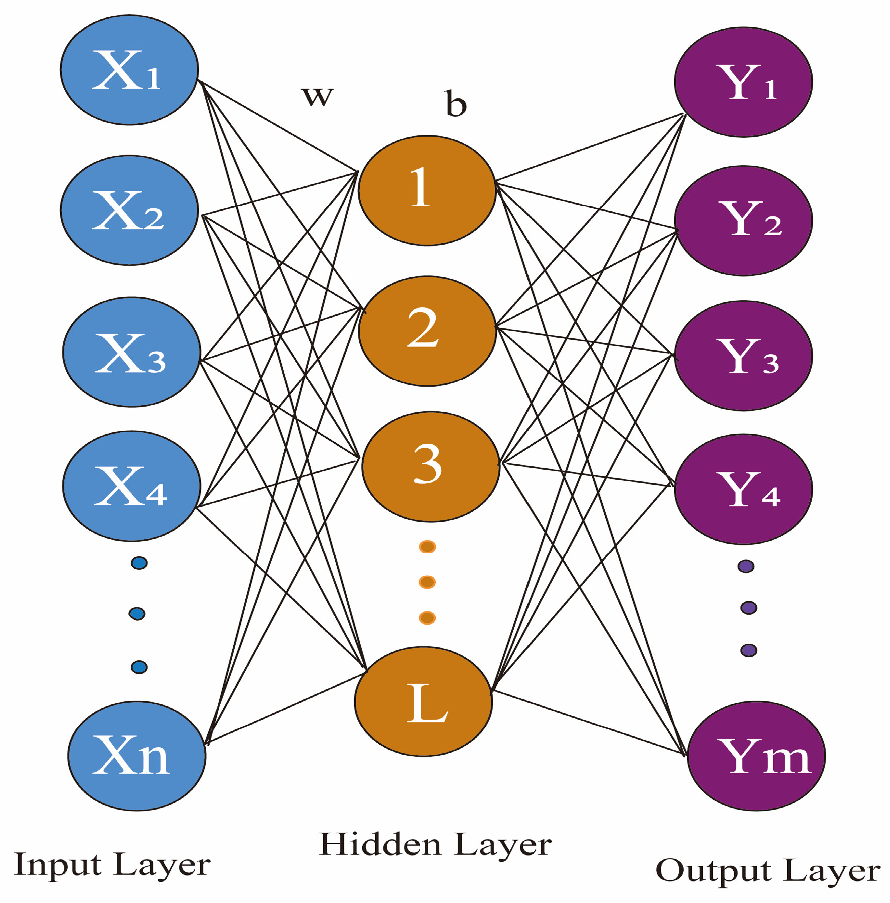
2.4.4. Construction and Evaluation of Inversion Model

The extreme learning machine (ELM) is a class of machine learning methods constructed on the basis of feedforward neural networks and has been widely applied in the field of remote sensing inversion [44]. However, when employing a pure ELM approach for regression prediction, issues such as low accuracy and significant errors persist [45]. Intelligent optimization algorithms, which are typically based on biological intelligence or physical phenomena, are stochastic search algorithms that do not generally require an objective function and constraints to be continuous or convex, and they can effectively address uncertainties in data. Therefore, employing intelligent optimization algorithms to optimize the ELM method can enhance inversion accuracy and reduce errors. The ELM is a single-hidden-layer feedforward neural network with randomization. As depicted in Figure 1, its model architecture consists of three layers: the input layer, the hidden layer, and the output layer. During training, the weights of the input layer and the biases of the hidden layer are usually obtained through random initialization. The training process is then completed by calculating the weights for the output layer. The weights of the input layer and the biases of the hidden layer have a significant impact on the ELM model. Optimizing these weights and biases can effectively improve the performance of the ELM. Consequently, this study selected dung beetle optimization (DBO), subtraction-average-based optimization (SABO), and the whale optimization algorithm (WOA) for algorithmic optimization.

• Dung Beetle Optimization (DBO)

The dung beetle optimization (DBO) algorithm is a novel swarm intelligence optimization algorithm inspired by the biological behaviors of dung beetles, including rolling, breeding, foraging, and stealing. It balances global exploration and local exploitation, offering advantages such as simple structure, strong adaptability, fast convergence, and high solution accuracy [45,46]. The process is as follows: First, the original anthocyanin data are input and randomly divided into training and testing sets, while the dung beetle population is initialized. Next, a fitness function is used to evaluate and rank the population’s adaptability. High-fitness positions are selected as starting points, and the beetles simulate behaviors like rolling, breeding, foraging, and stealing, updating their positions and fitness. The process continues until the maximum number of iterations is reached. Finally, the optimal input-layer weights and hidden-layer biases obtained from the DBO algorithm are applied to the ELM model for anthocyanin prediction.

2.

Subtraction-Average-Based Optimization (SABO)

The subtraction-average-based optimization (SABO) algorithm is an intelligent algorithm based on mathematical behaviors, capable of reducing the dimensionality of the input space and selecting effective features. It is known for its strong optimization capabilities and high convergence levels [47,48]. The algorithm begins with a random initialization of the population, setting the upper and lower bounds of the population range, and calculating the fitness values of different individuals. By comparing the fitness of new positions with that of old positions, the algorithm completes the optimization process.

3.

Whale Optimization Algorithm (WOA)

The whale optimization algorithm (WOA) is an efficient and straightforward metaheuristic optimization algorithm inspired by the hunting behavior of humpback whales [49]. By simulating the hunting strategies of humpback whales, such as encircling prey and the use of spiral-shaped bubble nets, WOA is capable of effectively searching across an entire solution space, thereby enhancing the algorithm’s global search capability [50].

Based on the impact of different supplementary lighting schemes on anthocyanin content, we sorted the samples in descending order of anthocyanin content and stratified them into three gradients. The average spectral curves of the purple-leaf lettuce under different lighting plans are shown in Figure 2. The samples were divided into a calibration set and a prediction set in a 2:1 ratio, with a calibration set of 90 samples covering different gradients of anthocyanin content, with 30 samples in each gradient (30 samples for each of the three lighting schemes: Plan 1, Plan 2, and no supplementary lighting). Additionally, there was a validation set of 45 samples, also covering different gradients of anthocyanin content, with 15 samples in each gradient (15 samples for each of the three lighting plans), as seen in

Table 1. Descriptive statistics of anthocyanin content (mg/g).

	Treatments	Number of Samples	Med	Min	Max	Sd	Cv%
Training Data	Supplementary Lighting Plan 1	90	0.106	0.062	0.153	0.027	25.9
	Supplementary Lighting Plan 2
	No Supplementary Lighting Plan
Testing data	Supplementary Lighting Plan 1	45	0.107	0.064	0.153	0.025	22.85
	Supplementary Lighting Plan 2
	No Supplementary Lighting Plan

Med: median; Min: minimum; Max: maximum; Sd: standard deviation; Cv: coefficient of variation.

. This model was first trained on the calibration dataset and then evaluated on an independent validation dataset to test its predictive accuracy and generalization ability.

The performance of the anthocyanin estimation model was evaluated using three metrics: the coefficient of determination (R²), the root mean square error (RMSE), and the relative prediction difference (RPD). In this study, the model with the highest R² and the lowest RMSE was considered the best, as these metrics have been proven effective in evaluating the performance of most models [51]. The calculation formulas for these metrics are as follows:

$${\mathrm{R}}^2={\displaystyle \frac{{\sum }_{\mathrm{i}=1}^{\mathrm{N}}\left[\mathrm{f}\right({\mathrm{x}}_{\mathrm{i}})-\overline{\mathrm{y}}]}{{\sum }_{\mathrm{i}=1}^{\mathrm{N}}[{\mathrm{y}}_{\mathrm{i}}-\overline{\mathrm{y}}]}}$$

(1)

$$\mathrm{R}\mathrm{M}\mathrm{S}\mathrm{E}={\displaystyle \frac{\sum _{\mathrm{i}=1}^{\mathrm{N}}{\left[\mathrm{f}\right({\mathrm{x}}_{\mathrm{i}})-{\mathrm{y}}_{\mathrm{i}}]}^2}{\mathrm{N}}}$$

(2)

$$\mathrm{R}\mathrm{P}\mathrm{D}={\displaystyle \frac{\mathrm{S}\mathrm{D}}{\mathrm{R}\mathrm{M}\mathrm{S}\mathrm{E}}}$$

(3)

where f(x_i), y_i, and $\overline{\mathrm{y}}$ are the predicted values, the observed values, and the average of the observed values of anthocyanins, respectively; N is the number of samples.

Based on this, the model evaluation was guided by the RPD values. An RPD value less than 1.0 indicated a very poor model, which was not considered, while an RPD between 1.0 and 1.4 suggested a poor model, capable only of distinguishing high and low values. An RPD between 1.4 and 1.8 indicated a fair model, suitable for evaluation and correlation analysis. When the RPD was between 1.8 and 2.0, it represented a good model, potentially capable of quantitative prediction, and an RPD between 2.0 and 2.5 indicated a very good model, suitable for quantitative prediction. Finally, an RPD greater than 2.5 denoted an excellent model, considered an outstanding quantitative model [52].

2.5. Data Analysis

Figure 3 shows the flowchart of the methodology used in this work. The figures involved in the spectral analysis and modeling method were drawn using the following software: MATLAB R2023a (Mathworks Inc., Natick, MA, USA) and Origin 2022 (OriginLab, Hampton, VA, USA).

3. Results

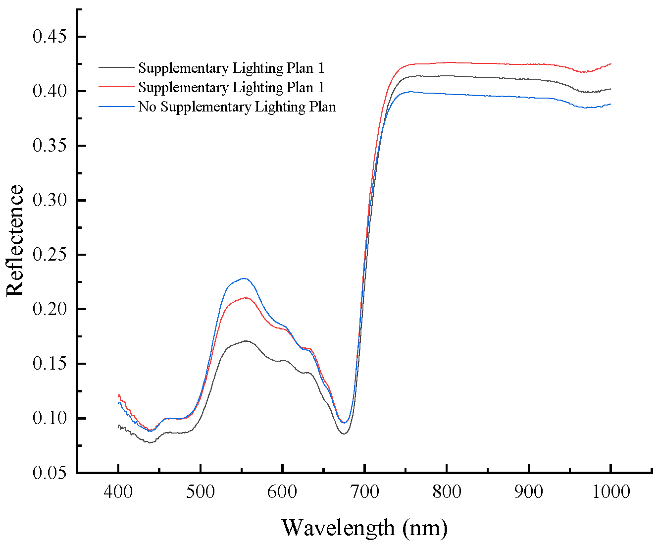
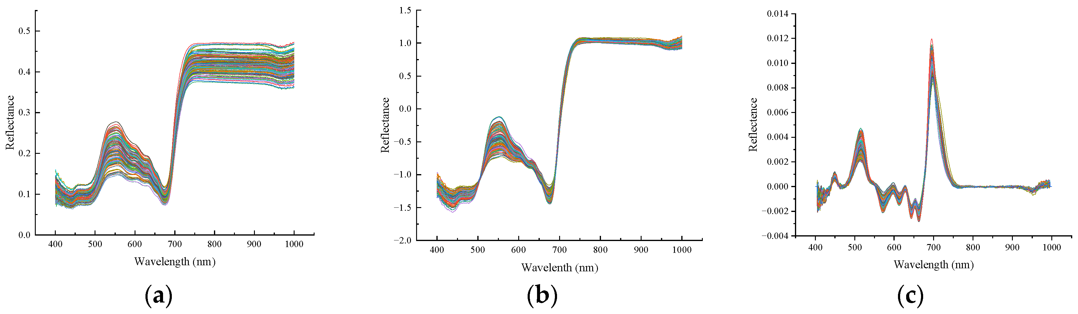
3.1. Spectra Pretreatment

We employed two preprocessing methods: the first-derivative (FD) and standard normal variate (SNV) methods, as shown in Figure 4.

3.2. Feature Extraction

Following the standard normal variate (SNV) preprocessing, the uninformative variable elimination (UVE) method was applied to eliminate uninformative variables from the original 601 bands. The stability distribution results of the UVE variables for the anthocyanins are shown in Figure 5a. The two parallel lines define the upper and lower limits of the variable stability. Wavelength variables that fell within these threshold boundary lines were excluded from further analysis, while those that exceeded the boundaries were retained for subsequent investigation. After UVE screening, a total of 66 wavelength variables were ultimately identified, accounting for 11% of the total wavelengths, as shown in Figure 5c. The process for the further screening of wavelengths with high-spectral characteristic related to the anthocyanin content based on CARS is illustrated in Figure 5b. Figure 5b illustrates the trends in the number of sampled variables, the root mean square error values, and the regression coefficient paths of the wavelengths as the number of samplings increased. After further screening by the CARS method following UVE, a final set of 12 wavelength variables was determined, representing 25.8% of the wavelengths after UVE screening and 2.8% of the total wavelengths, as shown in Figure 5d.

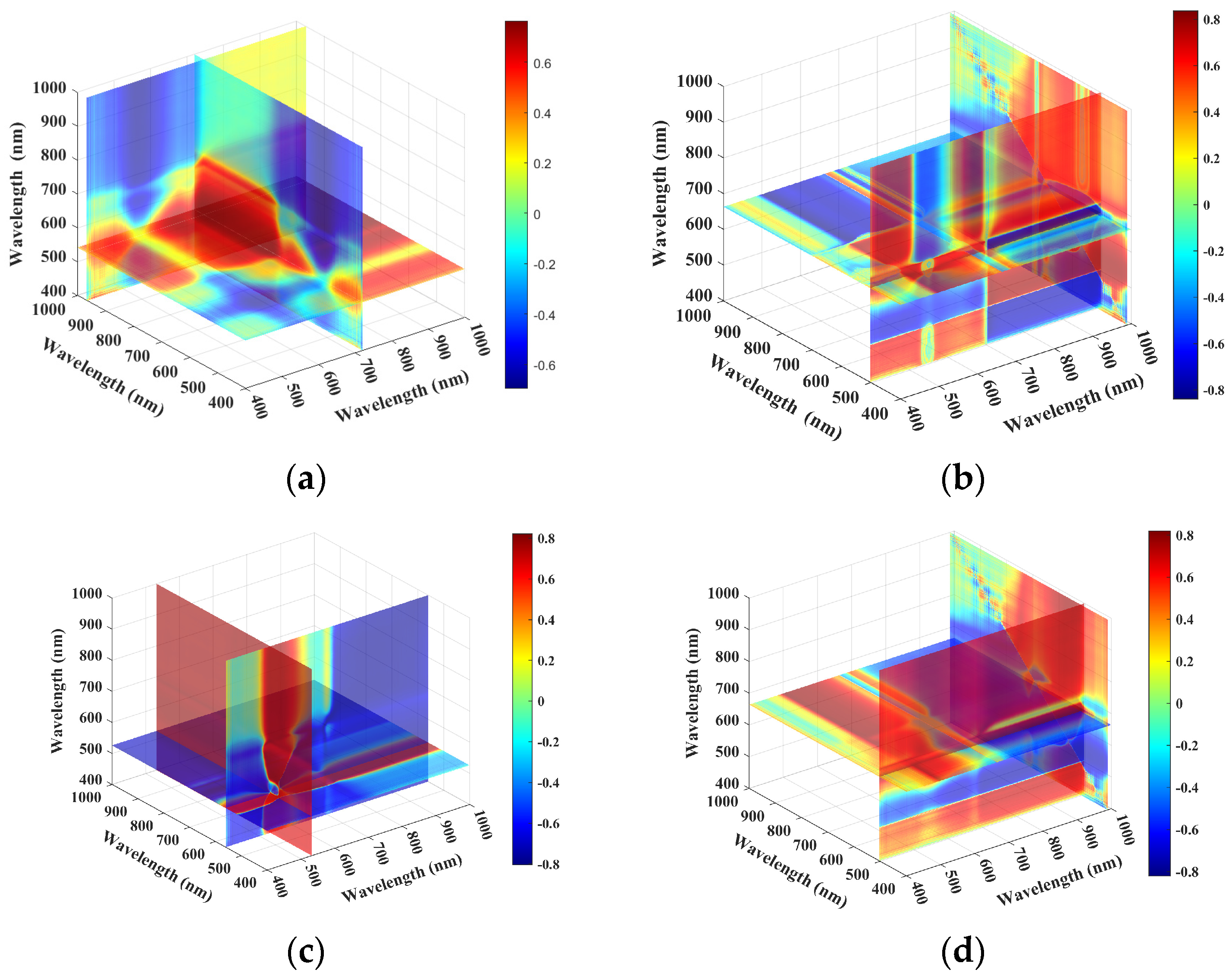
3.3. Constraction of Vegetation Indices

In this study, we selected two-band vegetation indices, including the NARI, MGRVI, ARI, and OSAVI, and three-band vegetation indices, including the MARI, EVI, TVI, PSRI, as anthocyanin-related vegetation indices, as shown in

Table 2. Vegetation indices.

Vegetation Index Type	Vegetation Index	Maximum Correlation Coefficient	Computational Formula	Wavelength Position	References
Two-band vegetation index	NARI	0.7902	(Ri−1 − Rj−1)/(Ri−1 + Rj−1)	(620 nm, 634 nm)	[53]
	MGRVI	0.7944	(Ri2 − Rj2)/(Ri2 + Rj2)	(703 nm, 532 nm)	[54]
	ARI	0.7676	Ri−1 − Rj−1	(532 nm, 697 nm)	[55]
	OSAVI	0.7976	1.16 × (Ri − Rj)/(Ri + Rj + 0.16)	(563 nm, 558 nm)	[16]
There-band vegetation index	MARI	0.7636	(Ri−1/Rj−1) × Rk	(542 nm, 966 nm, 720 nm)	[17]
	EVI	0.8345	2.5 × (Ri − Rj)/(Ri + 6 × Rj − 7.5 × Rk + 1)	(503 nm, 663 nm, 989 nm)	[56]
	TVI	0.8217	0.5 × (120 × (Ri − Rj) − 200 ×(Rk − Rj))	(526 nm, 560 nm, 532 nm)	[57]
	PSRI	0.8193	(Ri − Rj)/Rk	(664 nm, 503 nm, 989 nm)	[58]

. Heatmaps of the correlation coefficients between VI2, VI3, and the anthocyanins are shown in Figure 6 and Figure 7.

3.4. Anthocyanin Estimation Based on ELM Model and DBO-SABO-WOA Optimization

The optimal prediction models with characteristic wavelengths as input variables are shown in Figure 8, and the accuracy parameters of the models are presented in Figure 9. Under UVE feature extraction, for the FD preprocessing method, in the optimal group UVE + FD + SABO + ELM, the values of R_m² and R_v² were 0.8122 and 0.8035, respectively; the RMSE_m and RMSE_v were 0.0109 and 0.0117, respectively; and the RPD was 2.2814. For the SNV preprocessing method, in the optimal group UVE + SNV + DBO + ELM, the values of R_m² and R_v² were 0.8631 and 0.7986, respectively; the RMSE_m and RMSE_v were 0.0095 and 0.0123, respectively; and the RPD was 2.2533. The performance of the two preprocessing methods was comparable, with both slightly outperforming the optimal model of the raw data processing group (UVE + Raw + DBO + ELM), which had R_m² and R_v² values of 0.7919 and 0.7612, respectively; RMSE_m and RMSE_v values of 0.0114 and 0.0142; and an RPD of 2.0693. Under UVE + CARS feature extraction, for the FD preprocessing method, in the optimal group UVE + CARS + FD + SABO + ELM, the values of R_m² and R_v² were 0.84 and 0.8255, respectively; the RMSE_m and RMSE_v were 0.011 and 0.01, respectively; and the RPD was 2.4207. Under UVE + CARS feature extraction with the SNV preprocessing method, in the optimal group UVE + CARS + SNV + DBO + ELM, the values of R_m² and R_v² were 0.8623 and 0.8617, respectively; the RMSE_m and RMSE_v were 0.0098 and 0.0095, respectively; and the RPD was 2.7192. The SNV method performed the best among the two preprocessing methods, and both outperformed the optimal model of the raw data processing group, UVE + CARS + Raw + DBO + ELM, which had R_m² and R_v² values of 0.7329 and 0.7861, respectively; RMSE_m and RMSE_v values of 0.0136 and 0.0119; and an RPD of 2.1867. Observing the overall accuracy variations in the models in Figure 9, we find that the UVE + CARS + SNV + DBO + ELM model performed optimally. Additionally, for the raw-data ELM model, regardless of the preprocessing method and feature extraction method used, after optimization with the three DBO-SABO-WOA techniques, the model accuracy is improved.

The optimal prediction model using VI3 as the Input variable Is Illustrated In Figure 10, and the accuracy parameters of the models are presented in Figure 11. In the optimal group VI3 + WOA + ELM, the values of R_m² and R_v² were 0.8348 and 0.812, respectively; the RMSE_m and RMSE_v were 0.0109 and 0.011, respectively; and the RPD was 2.3323. The overall model’s accuracy surpassed that of the VI2 model, indicating that VI3 was more suitable for estimating anthocyanins. The parameters of the optimized ELM model were set as follows: a population size of 30, a maximum number of iterations of 500, and the activation function ‘sig’. The change in the fitness value of the optimal individual during the optimization process is shown in Figure 12. The fitness value of the UVE + SNV + CARS + DBO + ELM model reached its minimum of 0.8958 × 10⁻⁴ in the 243rd iteration and remained unchanged in the following iterations. The fitness value of the VI3 model reached its minimum of 0.121 × 10⁻⁴ in the 416th iteration and remained unchanged in the following iterations. For the raw-data ELM model, we also found that, regardless of which vegetation index was used to construct the model, the accuracy of the ELM, optimized using the three DBO-SABO-WOA techniques, showed improvements.

4. Discussion

4.1. Potential of Different Characteristic Wavelength Selection Methods in Estimating Anthocyanin Content of Lettuce

In order to reduce the impact of instrumental noise, baseline drift, and other factors on the raw spectra, two different spectral preprocessing methods, the FD and SNV, were analyzed. After SNV preprocessing, the R² of the UVE-CARS-SNV-WOA-ELM training set was 0.8623, with an RMSE of 0.0098. For the prediction set, the R² was 0.8617, the RMSE was 0.0095, and the RPD was 2.7192, as shown in Figure 8. The results show that the model performed well with good R² values, a low RMSE, and an RPD value greater than 2.5, indicating strong predictive ability. For example, studies show that using hyperspectral measurements with the random forest model can accurately estimate anthocyanin content in corn leaves (R² = 0.797; RMSE = 0.007; RPD = 2.24), helping assess corn’s physiological state under stress and supporting crop management and growth decisions [16]. The use of combined feature wavelength extraction (UVE-CARS) further enhanced the model’s prediction performance. Previous studies have shown that combined feature optimization methods can accurately and effectively determine optimal feature wavelengths. The UVE-SPA method has shown excellent performance in the robust quantification of tomato seedling vigor, optimizing spectral wavenumbers, reducing the dimensionality of spectral data, and improving the model’s predictive performance [59]. The CARS-SPA has demonstrated significant advantages in detecting reduced sugar content in potatoes [60] and predicting starch content in yellow corn [61], effectively improving the accuracy and efficiency of the models. UVE removes noise variables that do not contribute to the model by comparing the stability of regression coefficients between original and noise variables in PLS regression, thus eliminating ineffective wavelengths [21]. The CARS algorithm, inspired by the “survival of the fittest” principle in biological evolution, adaptively reweights and selects spectral bands, gradually eliminating redundant and less important bands [62]. UVE excels at eliminating non-informative variables, significantly reducing the complexity of datasets with redundant information [63]. In contrast, CARS focuses on iteratively reweighting to enhance the variables that contribute most to the model, making it more effective in preserving useful features [64]. By combining UVE and CARS, non-informative variables were first removed by UVE, and then CARS was used to further refine and optimize the feature selection, enhancing the model’s predictive accuracy and robustness. In the UVE-CARS approach, 12 feature variables were selected, accounting for 18.18% of the total UVE variables, as shown in Figure 5. The “filtering” followed by the “optimization” process of UVE-CARS effectively identified the key feature wavelengths across the entire spectral range, offering a novel approach for the rapid and accurate evaluation of anthocyanin content in lettuce.

4.2. Potential of Vegetation Indices in Estimating Anthocyanin Content of Purple Lettuce

For the optimal model based on the two-band vegetation index, the R² of the training set was 0.7907 and the RMSE was 0.0089 mg/g; the R² of the prediction set was 0.7133, the RMSE was 0.0117 mg/g, and the RPD was 1.8885. For the optimal model based on the three-band vegetation index, the R² of the training set was 0.8348 and the RMSE was 0.0109 mg/g; the R² of the prediction set was 0.812, the RMSE was 0.011 mg/g, and the RPD was 2.3323, as shown in Figure 10. Overall, the three-band model showed better predictive performance than the two-band model, as shown in Figure 11. In the application domain, two-band vegetation indices have been widely used in studies such as the estimation of the soybean leaf area index [30] and optimization of nitrogen nutrition diagnosis in winter rapeseed [29]. The three-band vegetation index has demonstrated stronger capabilities in predicting plant chlorophyll content [65], soil organic matter content [66], and leaf water content in spring wheat [67]. Studies have shown that the advantage of the three-band vegetation index lies primarily in its ability to utilize information from more bands, thereby enhancing the identification of plants’ physiological traits and improving estimation accuracy [68]. For example, when remote sensing imagery was used for estimating water transparency in the Yellow Sea, the three-band model provided better precision compared to the two-band model [69]. Furthermore, the three-band model was more sensitive to water content in spring wheat than single-band reflectance, as the spectral vegetation index converted simple reflectance data from individual bands into composite information from multiple bands. This approach improved spectral information extraction, minimized external influences, and maximized both the information load and band differentiation [67]. Therefore, the potential synergistic effect of the three-band combination results in better predictive performance for anthocyanin content.

4.3. Influence of Model Optimization in Estimating Anthocyanin Content of Purple Lettuce

The optimization results based on the model analysis indicated that, regardless of the feature extraction and preprocessing method used, the prediction results of the basic ELM model were relatively low, while the predictive performance of the three optimized models was significantly better, as shown in Figure 9 and Figure 11. The ELM model’s performance was optimized by the DBO, SABO, and WOA. The DBO algorithm achieved an improvement of 5.8–27.82%, the SABO algorithm improved by 2.92–26.84%, and the WOA showed a 3.75–27.51% improvement. The dung beetle optimization (DBO) algorithm, proposed by Xue et al. [70], is a swarm optimization technique known for its fast convergence speed and high precision [71]. Previous research has demonstrated that, compared to the SVM, ELM, and BPNN models, the DBO-ELM model exhibits superior prediction accuracy in the forecasting of rubber fatigue life [45]; the IDBO-ELM-based soft measurement model for BOD in wastewater treatment overcomes the randomness issue of the ELM model, significantly enhancing the model’s accuracy [72]. The proposed DBO-ELM model achieved high classification accuracy, surpassing the KNN, SVM, and ELM and BP by significant margins, demonstrating its potential in the wear-state recognition of abrasive clusters in an ordered grinding wheel [46]. Subtraction-average-based optimization (SABO), proposed by P. Trojovský and colleagues [73], is a heuristic optimization algorithm that guides search agents towards the global optimum through simple mathematical operations like averaging and subtraction in an iterative process. SABO has been used to optimize deep learning models for handling subgrade soil deformation under complex loading and freeze–thaw effects to improve pavement design and maintenance in cold regions [74], while also enhancing the performance of the back-propagation (BP) neural network for harmonic prediction, achieving high accuracy in forecasting harmonic voltage distortion and individual harmonic content [75]. The whale optimization algorithm (WOA) is a swarm intelligence algorithm inspired by the hunting behavior of whales [76]. Previous research has demonstrated the advantages of the WOA in improving the performance of the ELM in various fields, such as greenhouse gas emission prediction during subway construction [77], wine quality enhancement [78], lithium-ion battery life prediction [79], and microgrid fault detection and diagnosis [80]. In predicting crop yields, the ELM-WOA hybrid model outperforms standalone ELM, BP, SVM, and EMD-ELM models, achieving the smallest prediction error and highest accuracy [81]. Considering that the weights and thresholds of a basic ELM model are initialized randomly, which may lead to suboptimal parameters, DBO, SABO, and the WOA are employed to fine-tune the data weights and thresholds. The application of optimization methods to the ELM enhanced the anthocyanin prediction model, resulting in faster learning, an improved generalization ability, and higher recognition accuracy.

5. Conclusions

Monitoring anthocyanin levels in a timely manner is essential for evaluating the nutritional value of plants and assessing their growth conditions. By tracking these levels, it becomes possible to better understand plant health, optimize growth conditions, and improve crop management strategies. This study utilized hyperspectral technology to quantitatively detect anthocyanin content in purple-leaf lettuce. By applying two preprocessing methods and various wavelength selection techniques, the study aimed to develop a hyperspectral model with high predictive accuracy, providing a reference for using hyperspectral technology to measure anthocyanin content. The main conclusions are as follows:

(1)

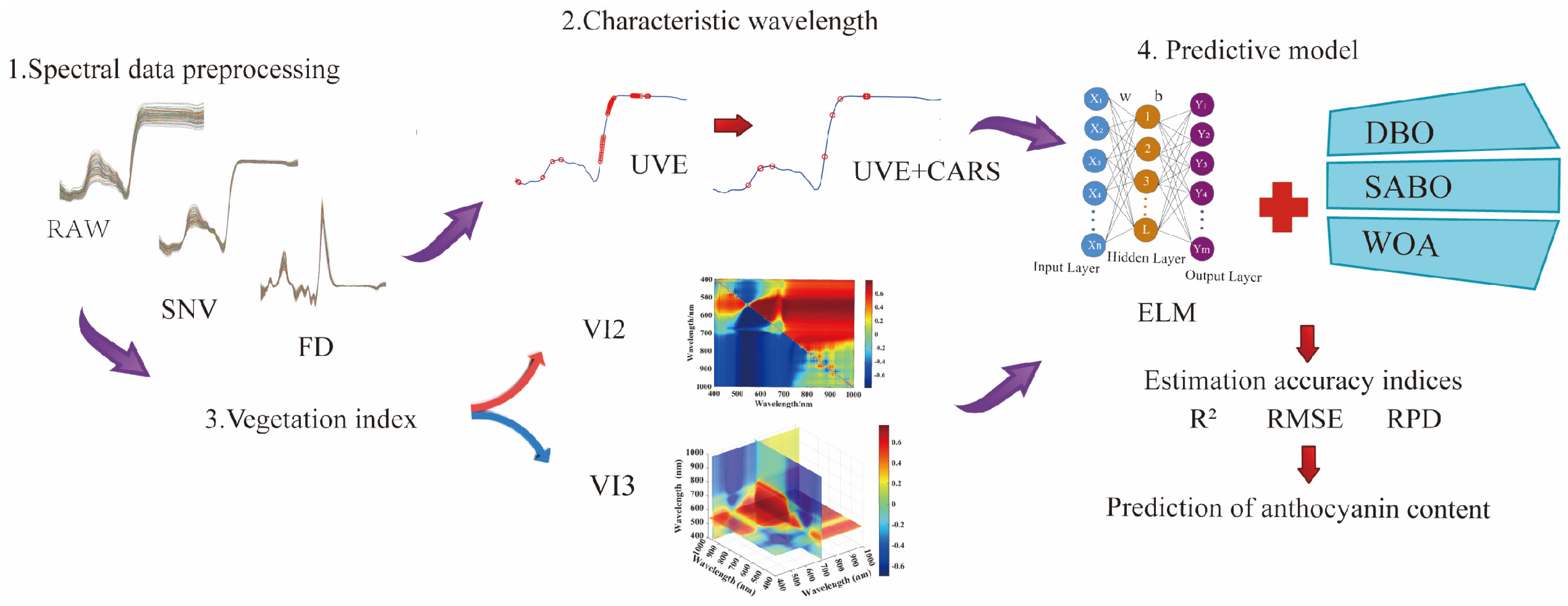
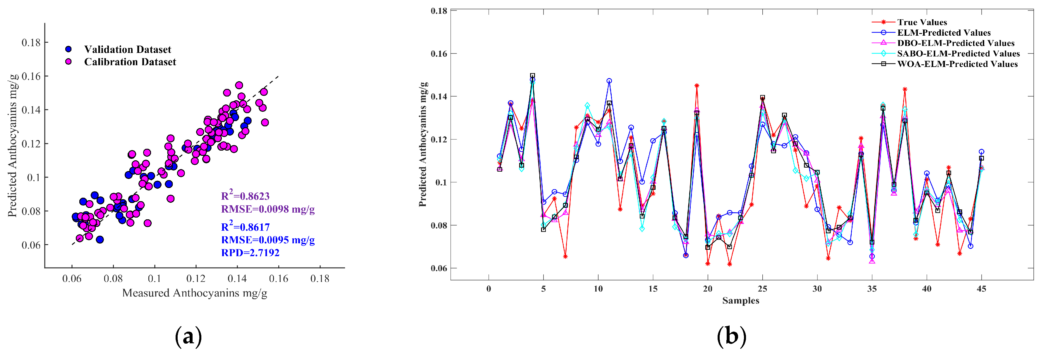
Two spectral preprocessing methods, the FD and SNV, were applied to reduce the impact of instrument noise, baseline drift, and other factors on the original spectra. The effects of feature wavelength selection methods, UVE and UVE-CARS, on the model performance were compared. The results indicated that UVE-CARS was the best variable selection method. The model built using the feature wavelengths selected by the UVE-CARS-SNV-DBO-ELM (R_v² = 0.8617; RMSE_v = 0.0095; RPD = 2.7192) achieved the best prediction performance for the anthocyanin content. In resource-constrained environments, UVE-CARS eliminates redundant features, thereby accelerating computation while preserving accuracy.

(2)

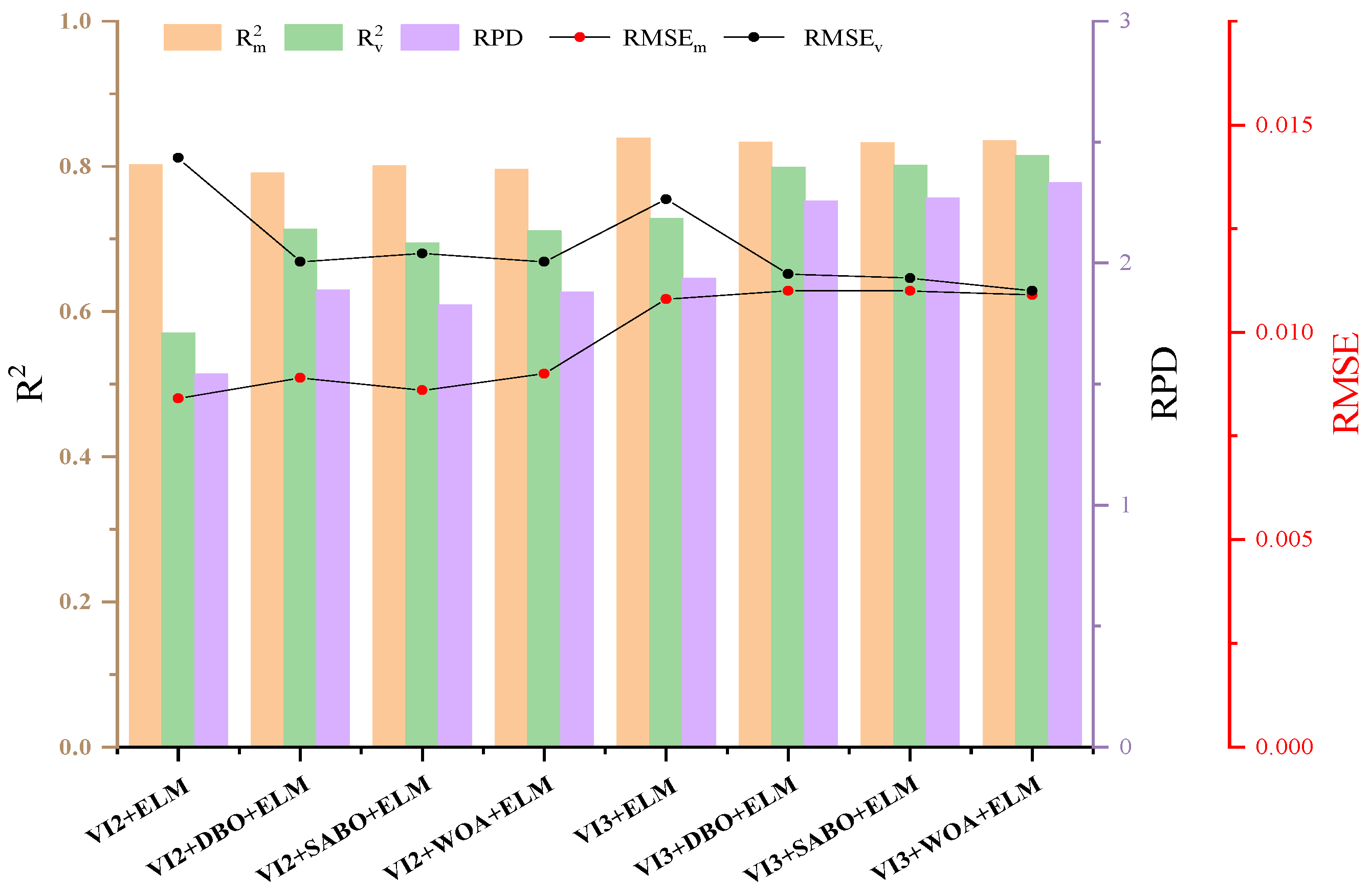
Based on the principle of the maximum correlation coefficient, two-band vegetation indices (NARI, MGRVI, ARI, OSAVI) and three-band vegetation indices (MARI, EVI, TVI, PSPR) were calculated. Compared to the prediction performance using two-band vegetation indices, the prediction performance using the three-band indices (R_v² = 0.812; RMSE_v = 0.011; RPD = 2.3323) was significantly improved.

(3)

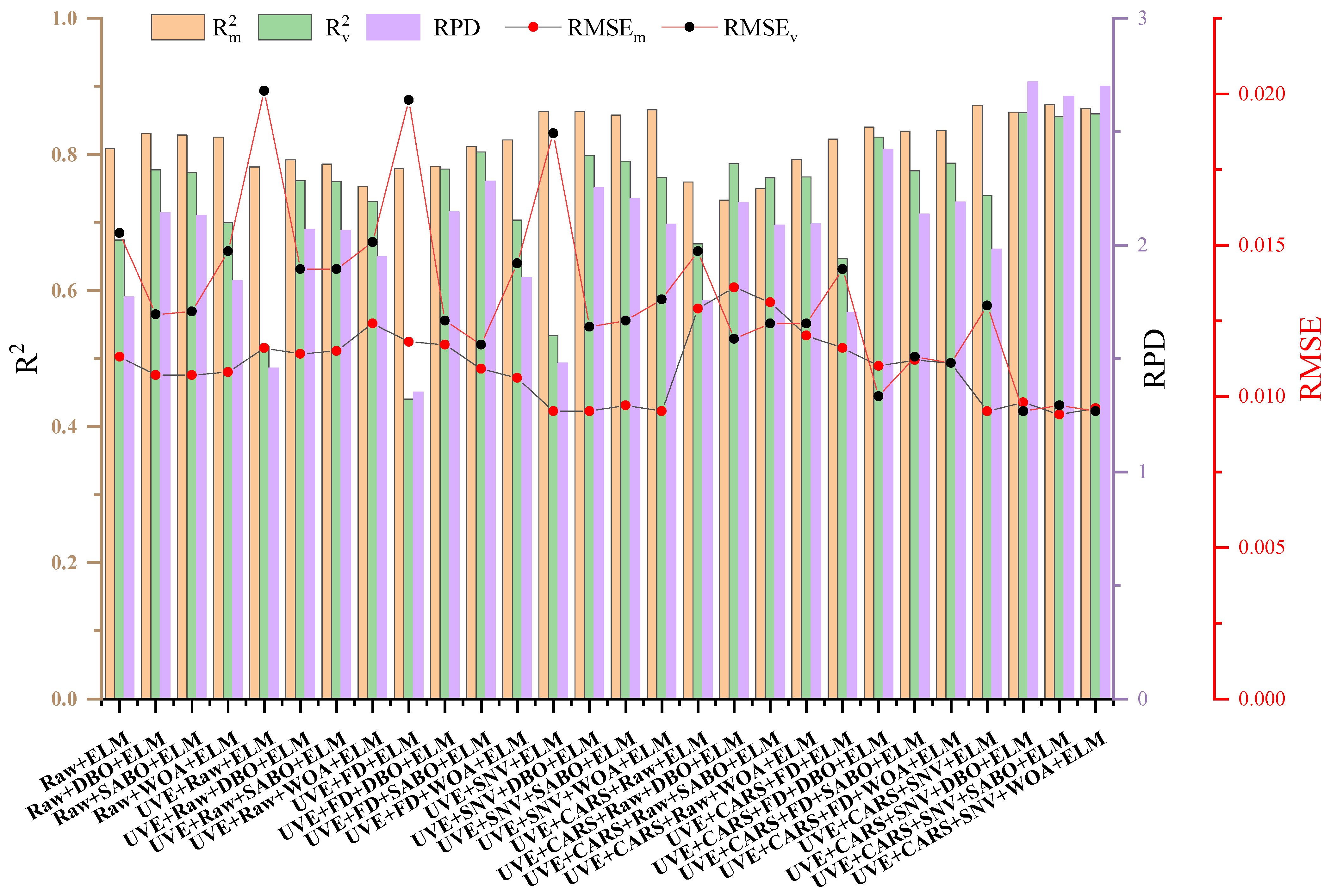
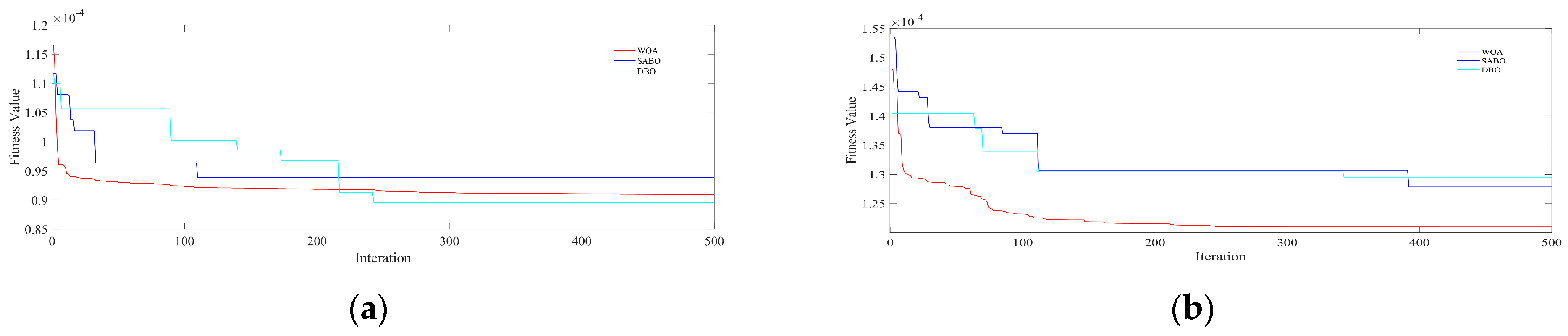
The performance of the ELM model was optimized using DBO, SABO, and the WOA. The DBO algorithm achieved an improvement in the R_v² ranging from 5.8% to 27.82%, the SABO algorithm showed an improvement from 2.92% to 26.84%, and the WOA demonstrated an improvement from 3.75% to 27.51% in the anthocyanin prediction. DBO, the WOA, and SABO optimize ELM weights and biases, balancing global and local searches to enhance performance and reduce computational costs. These techniques improve the feasibility of ELM models by maintaining high accuracy with lower resource requirements.

Hyperspectral technology shows potential for anthocyanin detection in agriculture but faces challenges like complex data processing, high costs, and low stability. Future efforts should optimize methods, reduce costs, and demonstrate economic benefits to encourage the adoption of such technology.

References

1. Perez-Lopez, U.; Sgherri, C.; Miranda-Apodaca, J.; Lacuesta, F.M.M.; Mena-Petite, A.; Quartacci, M.; Munoz-Rueda, A. Concentration of phenolic compounds is increased in lettuce grown under high light intensity and elevated CO2. Plant Physiol. Biochem. 2018, 123, 233–241. [Google Scholar] [CrossRef] [PubMed]
2. Khanam, U.K.; Oba, S.; Yanase, E.; Murakami, Y. Phenolic acids, flavonoids and total antioxidant capacity of selected leafy vegetables. J. Func. Foods 2012, 4, 979–987. [Google Scholar] [CrossRef]
3. Gould, K.S. Nature’s swiss army knife: The diverse protective roles of anthocyanins in leaves. J. Biomed. Biotechnol. 2004, 2004, 314–320. [Google Scholar] [CrossRef] [PubMed]
4. Shi, M.; Gu, J.; Wu, H.; Rauf, A.; Emran, T.B.; Khan, Z.; Mitra, S.; Aljohani, A.S.M.; Alhumaydhi, F.A.; Al-Awthan, Y.S.; et al. Phytochemicals, nutrition, metabolism, bioavailability, and health benefits in lettuce-a comprehensive review. Antioxidants 2022, 11, 1158. [Google Scholar] [CrossRef] [PubMed]
5. Dabravolski, S.A.; Isayenkov, S.V. The role of anthocyanins in plant tolerance to drought and salt stresses. Plants 2023, 12, 2558. [Google Scholar] [CrossRef]
6. Hu, Y.Z.; He, R.; Ju, J.; Zhang, S.C.; He, X.Y.; Li, Y.M.; Liu, X.J.; Liu, H.C. Effects of substituting b with fr and uva at different growth stages on the growth and quality of lettuce. Agronomy 2023, 13, 2547. [Google Scholar] [CrossRef]
7. Averina, N.; Savina, S.; Dremuk, I.; Yemelyanava, H.; Pryshchepchyk, Y.; Usatov, A. Influence of 5-aminolevulinic acid on physiological and biochemical characteristics of winter wheat varieties with different levels of anthocyanins in coleoptiles. Proc. Natl. Acad. Sci. Belarus Biol. Ser. 2022, 67, 135–146. [Google Scholar] [CrossRef]
8. Bhatt, V.; Sendri, N.; Swati, K.; Devidas, S.; Bhandari, P. identification and quantification of anthocyanins, flavonoids and phenolic acids in flowers of rhododendron arboreum and evaluation of their antioxidant potential. J. Sep. Sci. 2022, 45, 2555–2565. [Google Scholar] [CrossRef]
9. Singh, M.C.; Price, W.; Kelso, C.; Arcot, J.; Probst, Y. Measuring the anthocyanin content of the australian fruit and vegetables for the development of a food composition database. J. Food Compos. Anal. 2022, 112, 104697. [Google Scholar] [CrossRef]
10. Yu, Y.; Yu, H.Y.; Li, X.K.; Zhang, L.; Sui, Y.Y. Prediction of potassium content in rice leaves based on spectral features and random forests. Agronomy 2023, 13, 2337. [Google Scholar] [CrossRef]
11. Zhou, L.; Wu, H.B.; Jing, T.T.; Li, T.H.; Li, J.S.; Kong, L.J.; Zhou, L.N. Estimation of relative chlorophyll content in lettuce (Lactuca sativa L.) Leaves under cadmium stress using visible—Near-infrared reflectance and machine-learning models. Agronomy 2024, 14, 427. [Google Scholar] [CrossRef]
12. Eshkabilov, S.; Lee, A.; Sun, X.; Lee, C.W.; Simsek, H. Hyperspectral imaging techniques for rapid detection of nutrient content of hydroponically grown lettuce cultivars. Comput. Electron. Agric. 2021, 181, 105968. [Google Scholar] [CrossRef]
13. Feng, H.F.; Li, Y.X.; Wu, F.; Zou, X.C. Estimating winter wheat nitrogen content using spad and hyperspectral vegetation indices with machine learning. Trans. Chin. Soc. Agric. Eng. 2024, 40, 227–237. [Google Scholar]
14. Xu, T.Y.; Jin, Z.Y.; Guo, Z.H.; Yang, L.; Bai, J.C.; Feng, S.; Yu, F.H. Simultaneous inversion method of nitrogen and phosphorus contents in rice leaves using cars-run-elm algorithm. J. Agric. Eng. 2022, 38, 148–155. [Google Scholar]
15. Pandey, P.; Veazie, P.; Whipker, B.; Young, S. Predicting foliar nutrient concentrations and nutrient deficiencies of hydroponic lettuce using hyperspectral imaging. Biosyst. Eng. 2023, 230, 458–469. [Google Scholar] [CrossRef]
16. Jiang, S.Y.; Chang, Q.R.; Wang, X.P.; Zheng, Z.K.; Zhang, Y.; Wang, Q. Estimation of anthocyanins in whole-fertility maize leaves based on ground-based hyperspectral measurements. Remote Sens. 2023, 15, 2571. [Google Scholar] [CrossRef]
17. Kim, C.; van Iersel, M.W. Image-based phenotyping to estimate anthocyanin concentrations in lettuce. Front. Plant Sci. 2023, 14, 1155722. [Google Scholar] [CrossRef]
18. Liang, J.Q.; Liu, M.; Yu, K.; Liu, Z.L.; Kong, L.Q.; Hui, M.; Dong, L.Q.; Zhao, Y.J. Spectral pre-processing based on convolutional neural network. Spectrosc. Spectr. Anal. 2022, 1, 292–297. [Google Scholar]
19. Wang, W.D.; Chang, Q.R.; Wang, Y.N. Hyperspectral monitoring of anthocyanins relative content in winter wheat leaves. J. Trit. Crops 2020, 40, 754–761. [Google Scholar]
20. Zhang, M.L.; Chen, Y.J.; Wang, M.J.; Li, M.Z.; Zheng, L.H. A hyperspectral deep learning modelfor predicting anthocyanin contentin purple leaf lettuce. Spectrosc. Spectral Anal. 2024, 44, 865–871. [Google Scholar]
21. Liu, Y.H.; Wang, Q.Q.; Shi, X.W.; Gao, X.W. Hyperspectral nondestructive detection model of chlorogenic acid content during storage of honeysuckle. J. Agric. Eng. 2019, 35, 291–299. [Google Scholar]
22. Li, X.L.; Zhao, X.; Wei, F.F.; Peng, H.; Guo, H. Non-destructive prediction and visualization of anthocyanin content in mulberry fruits using hyperspectral imaging. Front. Plant Sci. 2023, 14, 1137198. [Google Scholar] [CrossRef] [PubMed]
23. Wang, Q.H.; Mei, L.; Ma, M.H.; Gao, S.; Li, Q.X. Nondestructive testing and grading of preserved duck eggs based on machine vision and near-infrared spectroscopy. J. Agric. Eng. 2019, 35, 314–321. [Google Scholar]
24. Zhang, H.Y.; Zhu, Q.B.; Huang, M.; Guo, Y. Automatic determination of optimal spectral peaks for classification of chinese tea varieties using laser-induced breakdown spectroscopy. Int. J. Agric. Biol. Eng. 2018, 11, 154–158. [Google Scholar]
25. Li, W.; Tan, F.; Zhang, W.; Gao, L.S.; Li, J.S. Application of improved random frog algorithm in fast identification of soybean varieties. Spectrosc. Spectral Anal. 2023, 43, 3763–3769. [Google Scholar]
26. Liu, Y.Y.; Wang, T.Z.; Su, R.; Hu, C.; Chen, F.; Cheng, J.H. Quantitative evaluation of color, firmness, and soluble solid content of korla fragrant pears via iriv and ls-svm. Agriculture 2021, 11, 731. [Google Scholar] [CrossRef]
27. Wei, X.; Zhang, Y.C.; Wu, D.; Wei, Z.B.; Chen, K.S. Rapid and non-destructive detection of decay in peach fruit at the cold environment using a self-developed handheld electronic-nose system. Food Anal. Methods 2018, 11, 2990–3004. [Google Scholar] [CrossRef]
28. Liang, K.; Liu, Q.X.; Pan, L.Q.; Shen, M.X. Detection of soluble solids content in ‘korla fragrant pear’ based on hyperspectral imaging and cars-iriv algorithm. J. Nanjing Agric. Univ. 2018, 41, 760–766. [Google Scholar]
29. Tang, Z.J.; Zhen, X.Y.; Xin, W.; Wei, Z.; Li, Z.J.; Zhang, F.C.; Chen, J.Y. Nitrogen nutrition diagnosis of winter oilseed rape using spectral indexes optimized by correlation matrix method. J. Agric. Eng. 2023, 39, 97–106. [Google Scholar]
30. Xiang, Y.Z.; Wang, X.; An, J.Q.; Tang, Z.J.; Li, W.Y.; Shi, H.D. Estimation of leaf area index of soybean based on fractional order differentiation and optimal spectral index. J. Agric. Mach. 2023, 54, 329–342. [Google Scholar]
31. Dai, F.S.; Shi, J.; Yang, C.S.; Li, Y.; Zhao, Y.; Liu, Z.Y.; An, T.; Li, X.L.; Yan, P.; Dong, C.W. Detection of anthocyanin content in fresh zijuan tea leaves based on hyperspectral imaging. Food Control 2023, 152, 109839. [Google Scholar] [CrossRef]
32. Cho, J.; Lim, J.H.; Park, K.J.; Choi, J.H.; Ok, G.S. Prediction of pelargonidin-3-glucoside in strawberries according to the postharvest distribution period of two ripening stages using vis-nir and swir hyperspectral imaging technology. LWT 2021, 141, 110875. [Google Scholar] [CrossRef]
33. Chen, S.S.; Zhang, F.F.; Ning, J.F.; Liu, X.; Zhang, Z.W.; Yang, S.Q. Predicting the anthocyanin content of wine grapes by nir hyperspectral imaging. Food Chem. 2015, 172, 788–793. [Google Scholar] [CrossRef] [PubMed]
34. Yue, R.; Yin, B.S.; Li, Z.F.; Lii, F.L. Monitoring of anthocyan in content of winter wheat infected by pst using uav rgb image. J. Triticeae Crops 2023, 43, 1–11. [Google Scholar]
35. Liu, X.Y.; Yu, J.R.; Liu, C.X.; Den, X.F. Estimation of anthocyanin content in prunus cerasifera based on color indices and bp neural network. J. Northwest For. Univ. 2022, 37, 145–152. [Google Scholar]
36. Guo, S.; Chan, Q.R.; Zhao, Z.Y.; Li, L.J.; Dong, Q.Q. Estimation of anthocyanin content in maize at different growth stages based on hyperspectral technology. Jiangsu Agric. Sci. 2024, 40, 303–311. [Google Scholar]
37. Miao, H.L.; Chen, X.K.; Guo, Y.M.; Wang, Q.; Zhang, R.; Chang, Q.R. Estimation of anthocyanins in winter wheat based on band screening method and genetic algorithm optimization models. Remote Sens. 2024, 16, 2324. [Google Scholar] [CrossRef]
38. Giusti, M.M.; Wrolstad, R.E. Characterization and measurement of anthocyanins by uv-visible spectroscopy. Curr. Protoc. Food Anal. Chem. 2001, F1–F2. [Google Scholar] [CrossRef]
39. Li, H.H.; Lu, W.; Hong, D.L.; Dang, X.J.; Liang, K. Rapid testing method of brown rice germination rate based on characteristic spectrum and general regression neural network. Laser Optoelectron. Prog. 2015, 52, 281–287. [Google Scholar]
40. Raju, C.S.; Løkke, M.M.; Sutaryo, S.; Ward, A.J.; Møller, H.B. Nir monitoring of ammonia in anaerobic digesters using a diffuse reflectance probe. Sensors 2012, 12, 2340–2350. [Google Scholar] [CrossRef]
41. Liu, Y.D.; Lin, X.D.; Gao, H.G.; Gao, X.; Wang, S. Quantitative analysis of chlorophyll content in tea leaves by fluorescence spectroscopy. Laser Optoelectron. Prog. 2021, 58, 444–453. [Google Scholar]
42. Wang, Q.H.; Zhou, K.; Wu, L.L.; Yun, W.C. Egg freshness detection based on hyper-spectra. Spectrosc. Spectral Anal. 2016, 36, 2596–2600. [Google Scholar]
43. Jiang, J.L.; Cen, H.Y.; Zhang, C.; Lyu, X.H.; Weng, H.Y.; Xu, H.X.; He, Y. Nondestructive quality assessment of chili peppers using near-infrared hyperspectral imaging combined with multivariate analysis. Postharvest Biol. Technol. 2018, 146, 147–154. [Google Scholar] [CrossRef]
44. Sun, J.; Yao, K.S.; Cheng, J.H.; Xu, M.; Zhou, X. Nondestructive detection of saponin content in panax notoginseng powder based on hyperspectral imaging. J. Pharm. Biomed. Anal. 2024, 242, 116015. [Google Scholar] [CrossRef] [PubMed]
45. Qin, W.; Li, C.G.; Pan, B.B.; Li, J.; Hu, J.T.; Ge, P.Z.; Liu, F.F. life prediction for vibration isolation rubber components based on dbo-elm model. Mech. Electr. Eng. Technol. 2024, 53, 13–19. [Google Scholar]
46. Guo, Y.; Chen, B.; Zeng, H.Y.; Qing, G.Y.; Guo, B. Research on wear state identification of ordered grinding wheel for c/sic composites based on dbo-elm. Wear 2024, 556–557, 205529. [Google Scholar] [CrossRef]
47. Zhang, Y.D.; Wang, Y.C. Study on elm power load forecasting metrics based on subtractive optimiser algorithm optimisation. Mod. Ind. Econ. Inform. 2024, 14, 124–126. [Google Scholar]
48. Liu, S.L.; Gao, Y.; Lin, R.C.; Tan, W.J. Improved subtraction-average-based optimization based on hybrid strategy. Intell. Comput. Appl. 2024, 14, 70–77. [Google Scholar] [CrossRef]
49. Liu, W.J.; Liu, Z.X.; Xiong, S.; Wang, M. Comparative prediction performance of the strength of a new type of ti tailings cemented backfilling body using pso-rf, ssa-rf, and woa-rf models. Case Stud. Constr. Mater. 2024, 20, e2766. [Google Scholar] [CrossRef]
50. Wang, N.; Chen, C.L.; Xiang, S.; Jin, Z.Y.; Bai, J.C.; Yu, F.H. Inversing chlorophyll contents in rice using radiation transport of leaf bilayer. Agric. Eng. J. 2024, 40, 171–178. [Google Scholar]
51. Osman, A.I.A.; Ahmed, A.N.; Huang, Y.F.; Kumar, P.; Birima, A.H.; Sherif, M.; Sefelnasr, A.; Ebraheemand, A.A.; El-Shafie, A. Past, present and perspective methodology for groundwater modeling-based machine learning approaches. Arch. Comput. Methods Eng. 2022, 29, 3843–3859. [Google Scholar] [CrossRef]
52. Viscarra Rossel, R.A.; Mcglynn, R.N.; Mcbratney, A.B. Determining the composition of mineral-organic mixes using uv–vis–nir diffuse reflectance spectroscopy. Geoderma 2006, 137, 70–82. [Google Scholar] [CrossRef]
53. Bayle, A.; Carlson, B.; Thierion, V.; Isenmann, M.; Choler, P. Improved mapping of mountain shrublands using the sentinel-2 red-edge band. Remote Sens. 2019, 11, 2807. [Google Scholar] [CrossRef]
54. Zhang, J.; Sun, B.; Yang, C.H.; Wang, C.Y.; You, Y.H.; Zhou, G.S.; Liu, B.; Wang, C.F.; Kuai, J.; Xie, J. A novel composite vegetation index including solar-induced chlorophyll fluorescence for seedling rapeseed net photosynthesis rate retrieval. Comput. Electron. Agric. 2022, 198, 107031. [Google Scholar] [CrossRef]
55. Gitelson, A.A.; Merzlyak, M.N.; Chivkunova, O.B. Optical properties and nondestructive estimation of anthocyanin content in plant leaves. Photochem. Photobiol. 2001, 74, 38–45. [Google Scholar] [CrossRef]
56. Fang, H.; Man, W.D.; Liu, M.Y.; Zhang, Y.B.; Chen, X.T.; Li, X.; He, J.N.; Tian, D. Leaf area index inversion of spartina alterniflora using uav hyperspectral data based on multiple optimized machine learning algorithms. Remote Sens. 2023, 15, 4465. [Google Scholar] [CrossRef]
57. Xing, N.C.; Huang, W.J.; Xie, Q.Y.; Shi, Y.; Ye, H.C.; Dong, Y.Y.; Wu, M.Q.; Sun, G.; Jiao, Q.J. A transformed triangular vegetation index for estimating winter wheat leaf area index. Remote Sens. 2020, 12, 16. [Google Scholar] [CrossRef]
58. Ren, S.L.; Chen, X.Q.; An, S. Assessing plant senescence reflectance index-retrieved vegetation phenology and its spatiotemporal response to climate change in the inner mongolian grassland. Int. J. Biometeorol. 2017, 61, 601–612. [Google Scholar] [CrossRef]
59. Ji, J.T.; Li, P.G.; Jin, X.; Ma, H.; Yong, L.M. Study on quantitative detection of tomato seedling robustness in spring seedling transplanting period based on vis-nir spectroscopy. Spectrosc. Spectral Anal. 2022, 42, 1741–1748. [Google Scholar]
60. Jiang, W.; Fang, J.L.; Wang, S.W.; Wang, R.T. using cars-spa algorithm combined with hyperspectral to determine reducing sugars content in potatoes. J. Northeast Agric. Univ. 2016, 47, 88–95. [Google Scholar]
61. Mu, W.Z.; Zhang, G.Y.; Zhang, W.; Yao, R.; Fu, N. Optimization of quantitative modeling of starch in huangshui based on near-infrared spectral feature extraction using competitive adaptive reweighted sampling combined with successive projections algorithm. Food Sci. 2024, 45, 8–14. [Google Scholar]
62. Ma, Z.L.; Wei, C.B.; Wang, W.H.; Lin, W.Q.; Nie, H.; Duan, Z.; Liu, K.; Xiao, X.O. Non-destructive prediction of anthocyanin concentration in whole eggplant peel using hyperspectral imaging. PeerJ 2024, 12, e17379. [Google Scholar] [CrossRef]
63. Chen, Y.Y.; Wang, X.C.; Zhang, X.L.; Sun, Y.; Sun, H.Y.; Wang, D.Z.; Xu, X. Spectral quantitative analysis and research of fusarium head blight infection degree in wheat canopy visible areas. Agronomy 2023, 13, 933. [Google Scholar] [CrossRef]
64. Zhu, Y.X.; Yu, L.; Hong, Y.S.; Zhang, T.; Zhu, Q.; Li, S.D.; Guo, L.; Liu, J.S. Hyperspectral features and wavelength variables selection methods of soil organic matter. Sci. Agric. Sin. 2017, 50, 4325–4337. [Google Scholar]
65. Gitelson, A.A.; Gritz, U.; Merzlyak, M.N. Relationships between leaf chlorophyll content and spectral reflectance and algorithms for non-destructive chlorophyll assessment in higher plant leaves. J. Plant Physiol. 2003, 160, 271–282. [Google Scholar] [CrossRef]
66. Zhang, Z.P.; Ding, J.L.; Wang, J.Z.; Ge, X.Y.; Li, Z.S. Quantitative estimation of soil organic matter content using three-dimensional spectral index: A case study of the ebinur lake basin in xinjiang. Spectrosc. Spectral Anal. 2020, 40, 1514–1522. [Google Scholar]
67. Nijat, K.; Zhang, Z.C.; Umut, H.; Zinhar, Z. Estimation of leaf water content of spring wheat based on 3d spectral index. J. Triticeae Crops 2024, 44, 522–531. [Google Scholar]
68. Li, X.C.; Zhang, Y.J.; Bao, Y.S.; Luo, J.H.; Jin, X.L.; Xu, X.G.; Song, X.Y.; Yang, G.J. Exploring the best hyperspectral features for lai estimation using partial least squares regression. Remote Sens. 2014, 6, 6221–6241. [Google Scholar] [CrossRef]
69. Yu, D.F.; Zhou, Y.; Xing, Q.G.; Ying, G.Y.; Zhou, B.; Fan, Y.G. Retrieval of secchi disk depth using modis satellite remote sensing and in situ observations in the yellow sea and the east china sea. Mar. Environ. Sci. 2016, 35, 774–779. [Google Scholar]
70. Xue, J.K.; Shen, B. Dung beetle optimizer: A new meta-heuristic algorithm for global optimization. J. Supercomput. 2023, 79, 7305–7336. [Google Scholar] [CrossRef]
71. Wu, C.L.; Fu, J.C.; Huang, X.; Xu, X.F.; Meng, J.H. Lithium-ion battery health state prediction based on vmd and dbo-svr. Energies 2023, 16, 3993. [Google Scholar] [CrossRef]
72. Du, X.J.; Yao, Y.P.; Qian, Q. Measurement modeling of wastewater treatment process based on idbo-elm. Ship Electr. Eng. 2024, 44, 103–107. [Google Scholar]
73. Trojovský, P.; Dehghani, M. Subtraction-average-based optimizer: A new swarm-inspired metaheuristic algorithm for solving optimization problems. Biomimetics 2023, 8, 149. [Google Scholar] [CrossRef]
74. Liu, X.W.; Li, J.; Liu, J.; Huang, C.; Liu, L.L. Prediction of permanent deformation of subgrade soils under f-t cycles using sabo-optimized cnn-bilstm network. Case Stud. Constr. Mater. 2024, 21, e3807. [Google Scholar] [CrossRef]
75. Lv, H.; Ling, W.; Zhu, Y.Z.; Du, W.L.; Liu, N.; Yang, D.M.; Cen, B.Y. prediction of power grid based on improved sabo-bp algorithm. Guangdong Electr. Power 2024, 37, 56–65. [Google Scholar]
76. Zhang, J.; Zhang, H.; Gao, X. Clustering routing algorithm for wsns based on fuzzy logic optimized by whale optimization algorithm. Inf. Control 2023, 52, 797–810. [Google Scholar]
77. Chen, Z.; Guo, Y.L.; Guo, C. Prediction of ghg emissions from chengdu metro in the construction stage based on woa-delm. Tunn. Undergr. Space Technol. 2023, 139, 105235. [Google Scholar] [CrossRef]
78. Dou, L.; Zheng, W.; Li, B.Q.; Li, F. Study on wine quality evaluation based on extreme learning machine improved by whale optimization algorithm. Food Mach. 2024, 40, 62–68. [Google Scholar]
79. Hao, R.; Wang, H.R.; Zhu, F.G. Indirect rul prediction of lithium-ion battery based on woa-delm. Control Instrum. Chem. Ind. 2023, 50, 37–43. [Google Scholar]
80. Lu, X.Q.; Li, C.A.; Wu, Z.Q. Microgrid fault diagnosis based on extreme learning machine optimized by whale algorithm. Smart Power J. 2022, 50, 15–21. [Google Scholar]
81. Yuan, S.Y. Prediction of grain yield model based on empirical mode decomposition and extreme learning machine. Comput. Mod. 2024, 3, 47–53. [Google Scholar]
Figure 1. Schematic diagram of extreme learning machine.
Agronomy 14 02915 g001
Figure 2. Average spectral curves of purple-leaf lettuce under different supplementary lighting plans.
Agronomy 14 02915 g002
Figure 3. A flowchart of the methodology.
Agronomy 14 02915 g003
Figure 4. Spectral preprocessing methods: raw spectra (Raw) (a), standard normal variate (SNV) (b), and first derivative (FD) (c).
Agronomy 14 02915 g004
Figure 5. Variables selected by UVE + CARS method. (a) Preliminary feature wavelengths selected by UVE. (b) Feature wavelengths further selected by CARS. (c) Feature wavelengths after initial UVE screening. (d) Final feature wavelengths after UVE + CARS screening.
Agronomy 14 02915 g005
Figure 6. Heatmaps of correlation coefficients between VI2 and anthocyanins. NARI (a), MGRVI (b), ARI (c), and OSAVI (d).
Agronomy 14 02915 g006
Figure 7. Heatmaps of correlation coefficients between VI3 and anthocyanins. MARI (a), EVI (b), TVI (c), and PSRI (d).
Agronomy 14 02915 g007
Figure 8. The optimal anthocyanin prediction model: UVE + SNV + CARS + DBO + ELM (a); the prediction errors of the test data (b).
Agronomy 14 02915 g008
Figure 9. The accuracy parameters of the models. Rm2 represents the training set’s R2, Rv2 represents the test set’s R2, RPD represents the residual predictive deviation, RMSEm represents the root mean square error of the training set, and RMSEv represents the root mean square error of the test set.
Agronomy 14 02915 g009
Figure 10. The optimal predicted anthocyanin values and measured values using VI3 (a); the prediction errors of the test data (b).
Agronomy 14 02915 g010
Figure 11. The accuracy parameters of the vegetation index models. Rm2 represents the training set’s R2, Rv2 represents the test set’s R2, RPD represents the residual predictive deviation, RMSEm represents the root mean square error of the training set, and RMSEv represents the root mean square error of the test set.
Agronomy 14 02915 g011
Figure 12. The fitness convergence curve of the UVE + SNV + CARS + DBO + ELM model (a) and the fitness convergence curve of the VI3 model (b).
Agronomy 14 02915 g012