Abstract
The application of intelligent mobile robots in agriculture has emerged as a new research frontier, with the integration of autonomous navigation technology and intelligent agricultural robots being the key to the widespread adoption of smart agricultural machinery. This paper investigates comprehensive coverage path planning for tracked lawnmowers within orchard environments and addresses challenges related to task allocation and battery life. Firstly, in this study, the motion model of the tracked lawnmower was initially simplified based on assumptions about the orchard environment. Force analyses were conducted on each of its motion mechanisms. For the known orchard environment, a grid-based mapping technique was employed to model the orchard environment. Then, in order to improve the algorithm speed and reduce the number of turns during the lawnmower’s traversal, the A* search algorithm was enhanced by combining the method of robot cluster traversal in the orchard environment. Finally, the improved method was simulated and verified in the MATLAB platform to investigate the influence of the number of lawnmower clusters on the path planning in the connected and non-connected orchards. Furthermore, two sets of on-site field trials were meticulously designed to validate the reliability, practicality, and efficacy of the simulation experiments.
1. Introduction
Traditional manual weeding is plagued by issues such as low labor efficiency, high production costs, and heavy workloads [1,2]. Therefore, mechanized weeding, particularly in conjunction with the emerging technology of robotic lawnmowers [3], is poised to become a primary solution. Robotic lawnmowers have the potential to alleviate labor burdens, reduce pesticide usage, protect orchard ecosystems, and enhance orchard productivity [4,5,6]. In the application of lawnmowers, the focal point of research lies in how to plan the travel paths of robotic lawnmowers. Commonly used path planning methods are categorized into traditional and intelligent approaches. Traditional path planning methods include free space methods [7], graph search methods, grid methods, and artificial potential field methods [8], whereas intelligent path planning methods are built upon theories such as genetic algorithms [9,10] and neural networks [11].
The problem of orchard traversal and coverage by robotic lawnmowers is an extension of path planning, falling under the umbrella of full-coverage path planning. Scholars have explored various methods for full-coverage path planning, with the A* algorithm having first been introduced by P. Hart, N. Nilsson, and B. Raphael in 1968 [12]. This algorithm, an enhancement of Dijkstra’s algorithm, incorporates a heuristic function, estimating the cost function value, to effectively search for the optimal path. However, it suffers from an abundance of expanded nodes and large turning angles during path search. T. Tsuji et al. proposed the artificial potential field method (APF) [13], treating the movement of robots in the environment as particles in a potential field to achieve obstacle avoidance and navigation. Nevertheless, in complex environments, the robot may fail to find a globally optimal path, and obstacle avoidance is less effective in densely populated obstacle layouts.
Moreover, integrating full-coverage path planning technology with a robotic swarm system [6] not only addresses issues of insufficient work capacity and poor fault tolerance in single-robot coverage but also adds flexibility to the task execution process, greatly improving work efficiency. In this context, ref. [14] combined a single-robot path planning algorithm with unit decomposition and heuristic search algorithms, proposing a multi-robot coverage planning method for floor-cleaning robots. Although this algorithm segmented the target area, it did not further investigate multi-robot task allocation. Refs. [15,16] introduced a heuristic function into the spanning tree algorithm and introduced a backtracking mechanism. This method was applied to multi-robot coverage path planning, enhancing robot coverage efficiency and algorithm robustness. However, it exhibits lower coverage efficiency when the starting points of the robots are unevenly distributed.
In the working scenario of a lawnmower cluster system, the problem of multi-robot collaborative task allocation is also a research hotspot [17]. Currently, multi-robot task allocation methods are mainly centralized, distributed [18], and hybrid, with corresponding algorithms including market mechanism-based allocation, linear programming-based task allocation, and swarm intelligence-based task allocation [19]. The market mechanism-based task allocation method proposed in [20] effectively addresses task allocation issues in dynamic or uncertain environments where a robot swarm works. However, it is not suitable for complex task scenarios in the system. The combinatorial auction-based task allocation method suggested in [21] resolves insoluble problems in task allocation and approximates the optimal solution. Still, this method typically involves a large number of combinatorial and auction processes, leading to high computational complexity, especially when the number of tasks and robots is large, impacting the real-time efficiency of the algorithm. The hybrid integer linear programming allocation method proposed in [21] can search for the optimal solution but exhibits lower allocation efficiency. Task allocation methods based on [22,23] address the issues of low task allocation efficiency and poor system scalability. When tackling the problem of multi-robot task allocation, swarm intelligence algorithms such as ant colony algorithms [24,25] or neural networks [26,27] exhibit high allocation efficiency, strong applicability, and ease of implementation, garnering significant attention from researchers [28].
Currently, there is relatively limited research by scholars on the path planning of orchard lawnmower robots, mainly focusing on flat areas and trimming fields of lawns. Furthermore, due to the overall large structure and high cost of lawnmower robots, their widespread application is constrained. This paper, set against the backdrop of cluster lawnmower operation, focuses on the traversal and coverage technology of cluster lawnmower robots in known orchard environments. It considers area decomposition and path planning under different constraints, analyzes the impact of different cluster lawnmower quantities on path planning, and identifies the optimal number of cluster lawnmowers for full-coverage path planning in the target area. The research objectives of this project are as follows:
- (1)
- To investigate the motion dynamics of a tracked lawnmower, this study simplifies its motion model based on specific assumptions regarding the orchard environment. Subsequently, a detailed force analysis is conducted on each individual motion mechanism. Employing a grid-based mapping technique, the known orchard environment is accurately modeled.
- (2)
- An improved A* algorithm is proposed to address existing issues in current lawnmower robot full-coverage path planning, thereby ensuring better traversal and coverage of the target area, with the lawnmower robot completely avoiding fruit trees and other obstacles during traversal. This paper validates the practicality of the improved algorithm through simulation experiments and field tests.
- (3)
- A comprehensive investigation is undertaken concerning the clustering of lawnmowers, involving an in-depth analysis of the influence of cluster quantity on path planning within both connected and non-connected orchards. The validation of simulation experiments is accomplished through meticulous field trials, ensuring the rigor of the research findings.
The remaining sections of this paper are organized as follows. Section 2 simplifies the motion model of the tracked lawnmower and conducts force analysis. The grid diagram method is used to model the known orchard environment. Section 3 introduces the task allocation method, which evenly distributes the workload based on the lawnmower robot’s energy capacity, and presents the improved A* path planning approach. In Section 4, simulations and on-site experiments are conducted to validate the improved A* path planning algorithm for varying numbers of lawnmower robots in the cluster. The performance of the proposed algorithm is assessed and analyzed. Finally, Section 5 summarizes and provides an outlook on the presented work.
2. Orchard Environmental Information Processing and Motion Analysis of Tracked Lawnmower
2.1. Orchard Environmental Information Rasterization
To ensure the accuracy of path planning, this paper employs a grid model to describe the two-dimensional workspace of the lawnmower robot, using binary information to represent orchard layout information. Initially, the grid size is determined, dividing the actual working environment into equally sized grid cells based on the cutting width of the lawnmower’s blade. Grid cells without obstacles are designated as white grids, indicating areas where the lawnmower can navigate. Grid cells with obstacles are represented as black grids, indicating areas the lawnmower must avoid and cannot traverse. The following assumptions are made:
- (1)
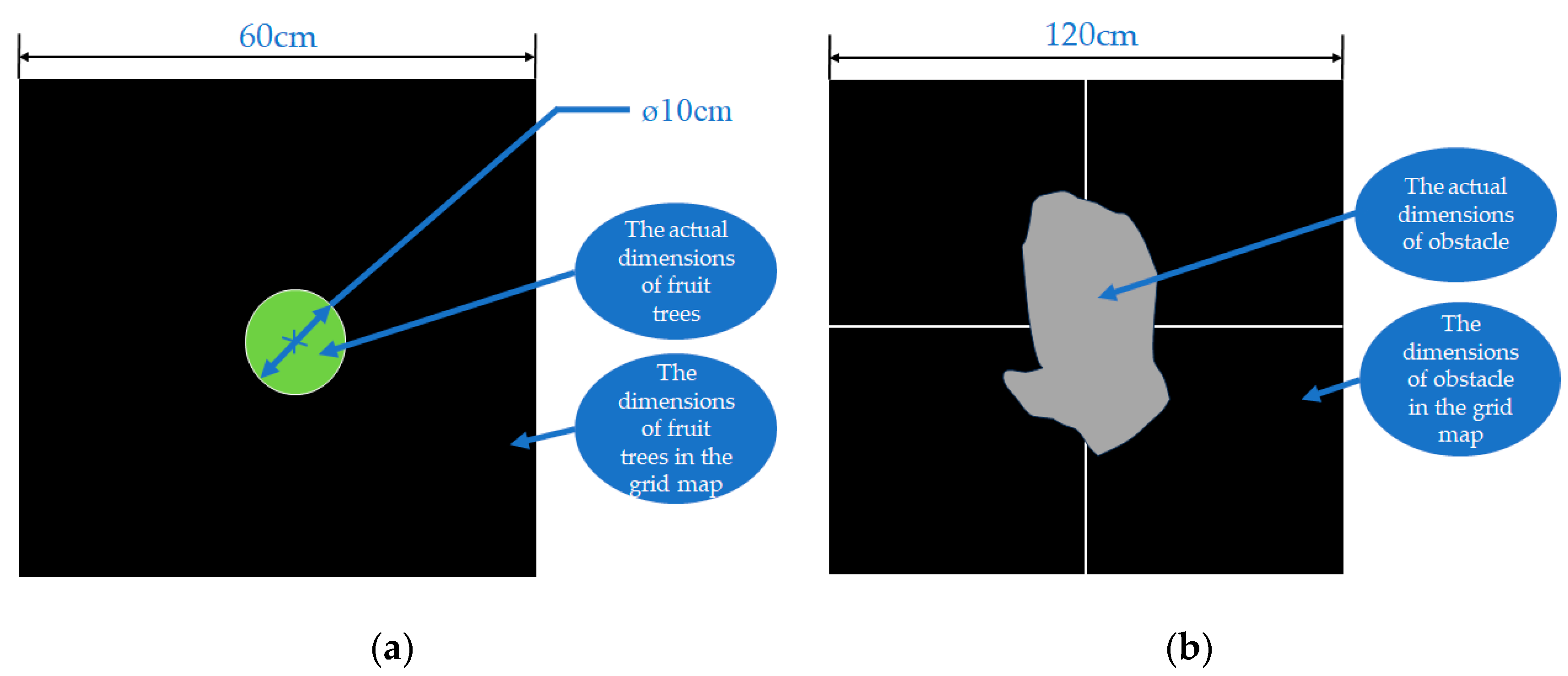
- As fruit trees within the orchard constitute the primary impediments in grid-based environmental modeling, requiring the lawnmower to navigate around them during operation, it is essential to represent obstacle dimensions in the grid map as larger than their real-world counterparts (employing fuzzy processing for modeling fruit trees). This entails incorporating a designated safety margin into the actual dimensions of obstacles within the environment (illustrated in Figure 1). Consequently, safety considerations are not imperative during operation of the lawnmower, and the lawnmower robot can be treated as a point mass while in motion.
- (2)
- Additional impediments within the orchard, such as large rocks and wells, similarly undergo fuzzy processing. In essence, obstacle dimensions in the grid map are magnified compared to their actual dimensions (as depicted in Figure 1).
- (3)
- In this study, the lawnmower robot operates solely within a two-dimensional workspace, and the impact of the lawnmower robot’s height is not considered.
- (4)
- The positions of fruit trees in the orchard are static, so the locations of obstacles on the grid map remain constant throughout the lawnmower robot’s movement.

Figure 1.
Actual dimensions of the object and its dimensions in the grid map. (a) Actual dimensions of fruit trees and their dimensions in the grid map; (b) actual dimensions of obstacles and their dimensions in the grid map.
Figure 1.
Actual dimensions of the object and its dimensions in the grid map. (a) Actual dimensions of fruit trees and their dimensions in the grid map; (b) actual dimensions of obstacles and their dimensions in the grid map.
On a two-dimensional plane, the orchard environment map where the lawnmower operates is divided into numerous equally sized grid cells. Each grid is annotated as 0 or 1 based on the presence of obstacles within the grid. In the grid map, the coordinates in the grid coordinate system can be correlated with latitude and longitude coordinates, resulting in more precise localization and thus enabling more accurate path planning. To objectively represent the grid-based environmental modeling, the following definitions are established:
Definition 1.
Target Workspace:
Definition 2.
Traversable Area:
where is the occupancy function:
The no-obstacles area can be further divided into the normal driving area, uphill area, downhill area, and overgrown grass area.
Definition 3.
Non-traversable Area:
Definition 4.
After the lawnmower starts working, grids that have been traversed and do not contain obstacles are labeled .
Definition 5.
The maximum length of the environmental map is denoted as , the maximum width is denoted as , and the dimensions (length and width) of each unit grid, denoted as , are equal to the mowing width of the lawnmower.
The grass-cutting robot requires effective paths to navigate in the simulated grid map. Therefore, it is necessary to define valid paths to enable the robot to move properly. During the journey from the starting point to the destination point, the point robot can move in eight directions: up, down, left, right, upper left, upper right, lower left, and lower right. The point robot is not allowed to cross over obstacles; any attempt to traverse through the center of an obstacle is considered an invalid path. Instead, the point robot must follow valid paths by maneuvering around obstacles and moving into adjacent grid cells.
2.2. Motion Analysis of Tracked Lawnower
When establishing the motion model of the tracked lawnmower, the ground environment of the orchard should be considered first, taking into account the area of contact between the tracks and the ground. Simultaneously, it is necessary to confirm the operational state of the tracked lawnmower. In this study, the focus is primarily on establishing a motion model for the steady-state movement of the tracked lawnmower in orchards located in hilly and mountainous areas. Therefore, the following conditional assumptions are made:
- (1)
- Orchards in hilly regions mainly refer to those planted on undulating, continuous low hills. These orchards have an absolute height of 500 m, and the relative height does not exceed 200 m. Among them, orchard terrains with slopes of less than 15 degrees, such as flat or gently sloping areas, are suitable for mechanized cultivation and planting. However, when the slope of the orchard terrain exceeds 25 degrees, mechanized operations in the orchard become challenging. Therefore, it is assumed that the tracked lawnmower operates on slopes between 0 and 15 degrees, and the unevenness of the orchard ground is not considered.
- (2)
- The assumption is made that the tracked lawnmower behaves as a rigid body during its motion.
- (3)
- Deformation of the rubber tracks during motion and changes in track tension are not considered.
In this study, the walking model of the tracked lawnmower adopts a crawler walking mechanism. The main components constituting the crawler walking mechanism are the bogies on both sides of the tracked lawnmower. These bogies consist of a bogie frame and a “four-wheel and one-belt” arrangement (as shown in Figure 2). During operation of the lawnmower, the tracks come into direct contact with the soil. At this point, the weight of the tracked lawnmower is primarily supported by the supporting wheels. When the driving wheel operates, the tracks undergo a winding motion relative to the bogie frame.

Figure 2.
Tracked lawnmower bogie mechanism.
The overall structure of the tracked lawnmower is primarily composed of two systems: the chassis and the track, forming a complex multibody system. When the lawnmower travels on a certain slope without undergoing steering or pitching motion, both the frame and the tracks undergo translational motion, while the wheels undergo rotational motion. Therefore, when calculating the energy of the lawnmower, it needs to be simplified into a multibody model. When the lawnmower is working in an orchard and does not undergo steering motion, in order to ensure that the lawnmower continues to travel in the given direction along a specified path, coordinate is created for the given path. Thus, the motion of the lawnmower is subject to the following constraints:
where represents the relative sliding rate between the lawnmower’s track and the ground, denotes the radius of the drive wheel, and represents the angular velocity of the drive wheel.
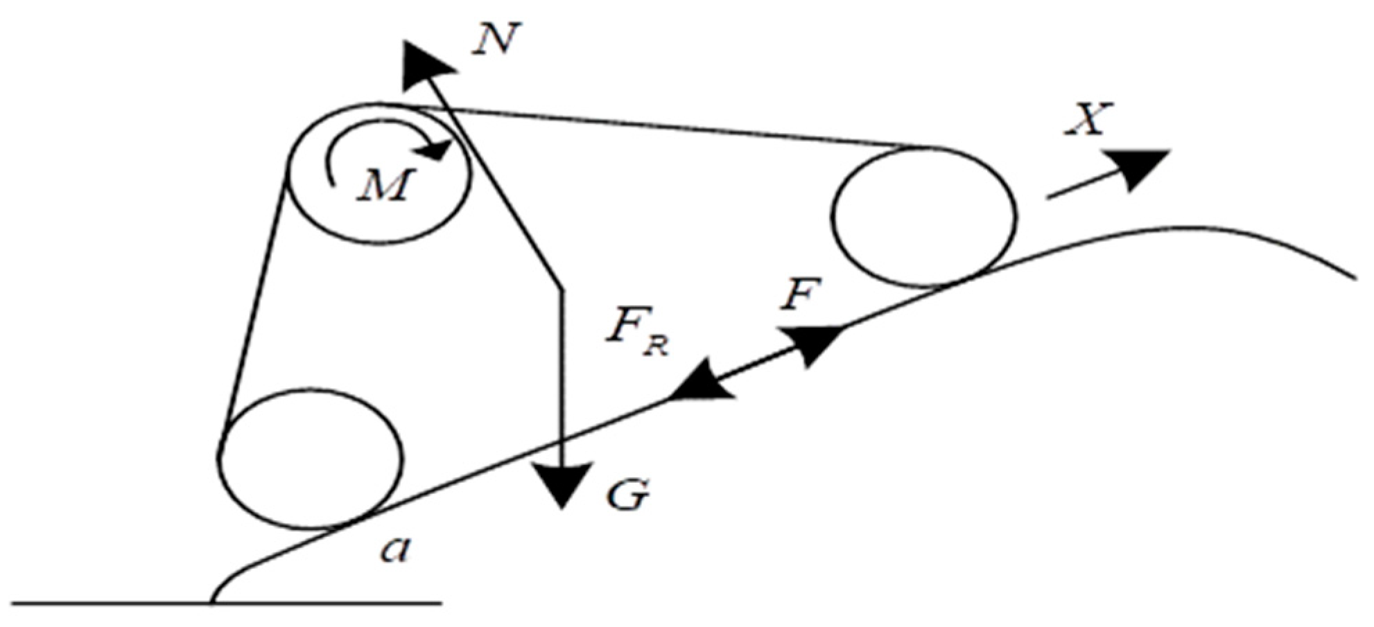
The resistance encountered by the lawnmower during motion includes acceleration resistance , air resistance , rolling resistance , and slope resistance . Due to the relatively low speed of the lawnmower during movement in the orchard, the impact of air resistance is not considered in this study. Assuming that the road conditions and forces acting on the lawnmower are symmetrical during travel, the forces on the tracks and the motion of the tracks are also symmetrical. For force analysis, one track is selected (as shown in Figure 3).
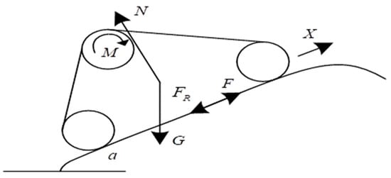
Figure 3.
Force analysis of the lawnmower tracks.
In Figure 3, N is the vertical reaction force from the ground to the lawnmower, G is the weight of the lawnmower itself, and m is the mass of the lawnmower. Assuming that the motor of the lawnmower imparts a driving torque M to the drive wheel, the rated power of the motor is P, and the transmission efficiency of the motor is , then the driving force of the lawnmower is given by:
where represents the coefficient for the conversion of motor power output to mechanical force.
During the driving process, the lawnmower undergoes translational motion due to its own mass, resulting in a translational component . The rotational component generated by the acceleration and deceleration of rotating components in the lawnmower is given by:
where , , and constitute the acceleration resistance of the lawnmower during travel, where represents the acceleration of the lawnmower along the x-direction. represents the inertia torque generated by the non-uniform motion of rotating components, and I is the total equivalent rotational inertia generated by all non-uniformly moving rotating components of the lawnmower.
To simplify the analysis process, considering equal masses for the tracks borne by each wheel, then:
where is the radius of each wheel, is the radius of each wheel, is the mass of the track, n is the number of wheels, and the transmission coefficient ratio is . The rotational component is then given by:
The total resistance during mowing operation is:
Under rated conditions, the motor will experience a certain torque loss , where is the rated speed of the motor. The magnitude of the torque loss is related to the speed. Assuming is a constant and s is the slip ratio, the transmission efficiency is given by . When the slip ratio s = 0, the loss force during the lawnmower’s travel is:
For a given path, the lawnmower is studied as a whole during the travel process since the system has only one degree of freedom. As the system only has one degree of freedom, the velocity v = x. While the lawnmower is traveling in the orchard, apart from the tracks and wheels, the other components undergo translational motion. Therefore, the velocities of these components are the same, i.e., . The total energy of the system includes the translational kinetic energy , rotational kinetic energy , gravitational potential energy , and torsion spring elastic potential energy . The total energy of the lawnmower system is expressed as:
where is the rotational inertia of the wheel and track system, and is the torsion angle of the spring.
The Lagrange equation for the system is given by:
where is the loss force, is the active generalized force, and L, Q, and are substituted into the Lagrange equation to obtain the motion differential equation:
where , , , and .
Integrating the above equations, the kinematic equation for the tracked lawnmower in orchard travel is obtained as:
where and are constants. Assuming the initial travel conditions for the lawnmower are t = 0, x = 0, and and substituting them into the equation, the results are: , .
Therefore, the velocity of the tracked lawnmower in orchard travel is given by:
3. Clustered Lawnmower Task Allocation and Path Planning Methods
3.1. Problem Description and System Framework
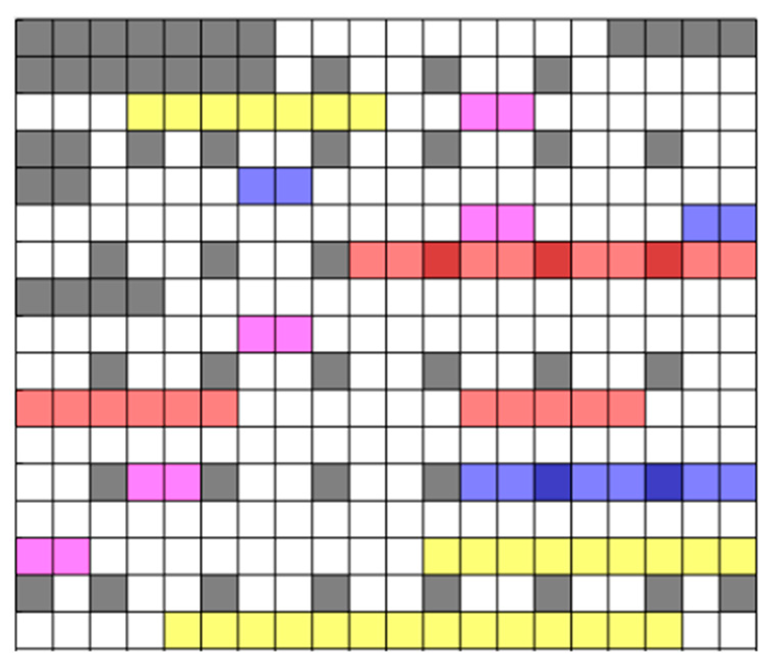
For the path planning of multiple lawnmowers in the orchard, a global path planning approach is employed based on the known external working environment. This paper focuses on planning the movement paths of tracked lawnmowers in a two-dimensional plane and employs a grid-based mapping method to create a simulated working environment for the lawnmowers (as shown in Figure 4), comprising M*N grid cells.

Figure 4.
Robotic simulated working environment. (White grids represent grids where the lawnmower can travel, gray grids indicate obstacle grids (i.e., impassable grids), pink grids represent uphill areas, blue grids denote down-hill areas, red grids represent overgrown grass areas, and yellow grids represent areas with sparse weeds.)
In Figure 4, white grids represent grids where the lawnmower can travel, gray grids indicate obstacle grids (i.e., impassable grids), pink grids represent uphill areas, blue grids denote downhill areas, red grids represent overgrown grass areas, and yellow grids represent areas with sparse weeds. The positions of obstacles on the grid map are fixed. In this section, the working area is divided into subareas, and each subarea is assigned to individual lawnmowers based on specific constraints. This allocation strategy ensures efficient obstacle avoidance as the lawnmowers execute their tasks.
In this section, the research on lawnmowers and orchard environment is characterized by the following two points:
- (1)
- The lawnmowers in the cluster are homogeneous robots, meaning each lawnmower carries the same amount of energy.
- (2)
- The environmental information of the orchard is known. The positions of the trees and other obstacles in the orchard are fixed and unchanging, and there are no dynamic obstacles in the orchard.
The problem of orchard traversal coverage for the cluster of lawnmowers can be summarized as a multi-robot task allocation problem in obstacle environments. This includes constructing the environmental map, decomposing and assigning target areas, and planning subregion paths.
Subsequently, a mathematical description of the complete coverage path planning is presented. The lawnmower operates within a two-dimensional bounded environment. The lawnmower’s specific location in the real environment can be represented using coordinates (x, y) in a two-dimensional coordinate system, denoted as follows:
To indicate the specific status of each grid in the simulated environmental map, the function is defined. When , it indicates that the area is a grass-covered region in the orchard, which means it is the area that the lawnmower robot needs to traverse (the traversable area), and it can be represented as: . When , it indicates that this grid is either an obstacle area or an area where fruit trees are planted, which means it is an area that the lawnmower robot does not need to traverse (non-traversable area), and it can be represented as: . The geometric relationship among the environmental map region , the area that the lawnmower robot needs to traverse , and the area that the lawnmower robot does not need to traverse can be described as follows: .
In this way, the travel path of the lawnmower robot in the orchard environment is composed of the trajectories of each point traversed by the lawnmower robot in the covered area , represented by the set :
where represents the path traveled by each lawnmower robot to completely traverse a subregion of the covered area, the coordinates are the starting positions of the lawnmower, and the coordinates are the endpoints for each lawnmower’s travel, so each lawnmower’s travel path is a sub-path of .
3.2. Target Area Decomposition
In this section, the optimal travel direction for the lawnmower is determined. One of the factors that must be considered in the full-coverage path planning problem is the turning situation of the lawnmower while traveling. To reduce the lawnmower’s working time and its energy consumption, it is necessary to minimize the number of turns the lawnmower makes. Therefore, determining the direction in which the lawnmower traverses is aimed at reducing the total working time and conserving the overall energy of the lawnmower.
The optimization objective is to reduce the total working time and energy consumption of the lawnmower. Therefore, the direction with the minimum number of turns for the lawnmower is chosen as the optimal travel direction. To determine the lawnmower’s travel direction, a common approach is to traverse and identify the minimum width direction of the area of the orchard to be covered. Subsequently, the vertical direction of the orchard’s minimum width direction is chosen as the lawnmower’s optimal travel direction. The specific steps are as follows:
- (1)
- Place the lowest point of the convex polygon representing the area to be covered at the x-axis of the two-dimensional coordinate system, ensuring that the y-coordinate of this lowest point is 0.
- (2)
- Rotate the polygon while maintaining its lowest point on the x-axis. Simultaneously, measure the height of the polygon in real time, i.e., the y-coordinate value of the highest point of the polygon.
- (3)
- Select the direction with the smallest y-coordinate value for the highest point of the polygon, which corresponds to the minimum width direction of the convex polygon. This direction determines the optimal travel direction for the lawnmower, which is the angle in the vertical direction from the x-axis to the minimum width direction of the convex polygon, as illustrated in Figure 5, which represents the search process.
 Figure 5. Determination of the optimal travel direction using a traversal search method. (The blue dash line is the height of each polygon, where the minimum value is the best driving direction.)
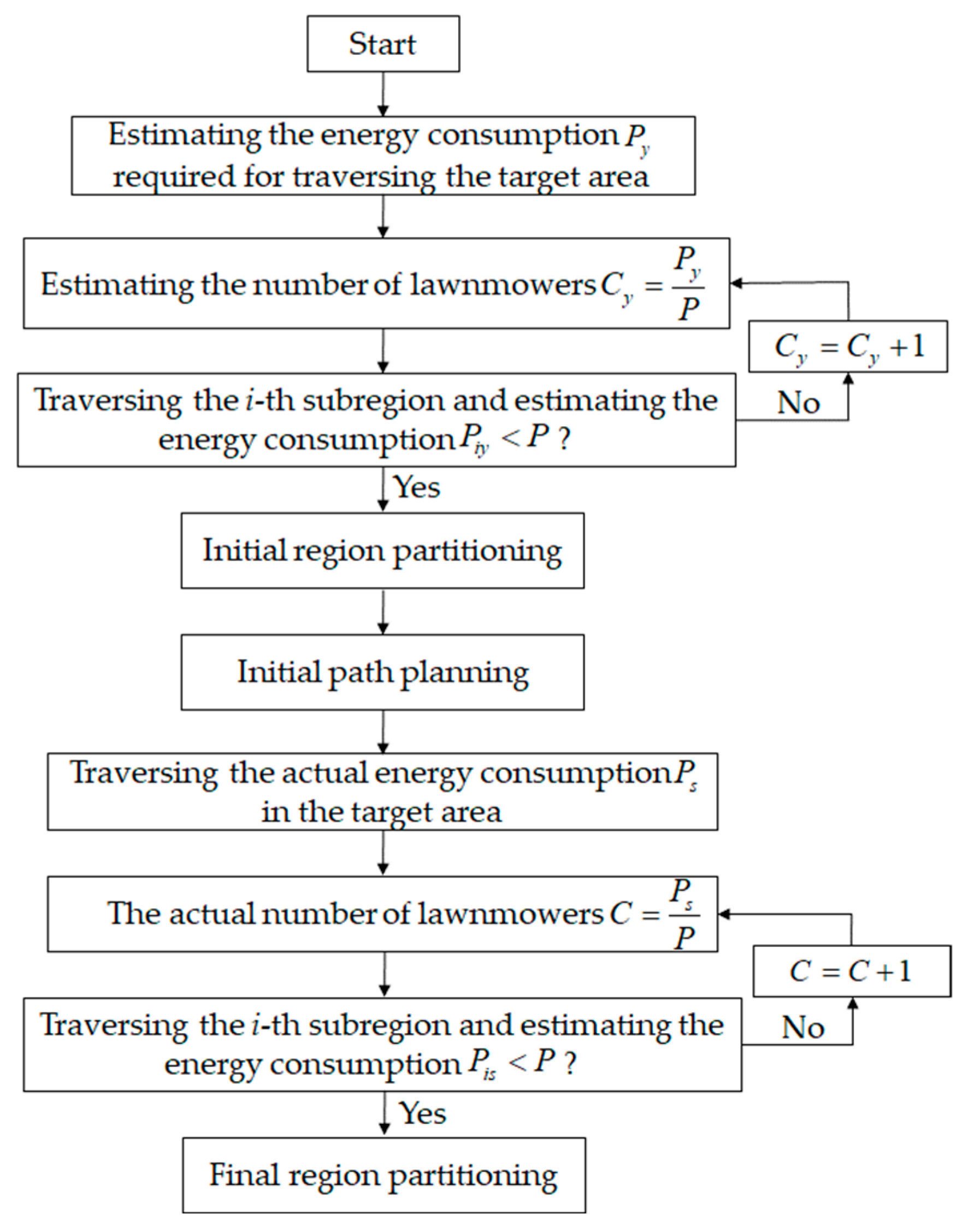
Partitioning the target area into multiple subareas is a prerequisite for task allocation. Rationally dividing the target area into subareas can reduce the problem of unsolvable task allocation and enhance the efficiency of robot task completion, improving system robustness. For the case of grass-cutting robots traversing the orchard for weed control, how to partition the area of the orchard waiting to be covered into corresponding subareas based on the robot’s available energy is critical for solving the allocation problem. In this study, the proposed models for estimated energy consumption and actual energy consumption are introduced to constrain the subdivision of subareas. Estimating energy consumption calculates the total energy consumed by the lawnmower while traversing each row of the grid map. During the traversal process, the lawnmower may revisit certain grid cells, and actual energy consumption includes the cost of revisiting these cells in addition to the estimated energy consumption. The specific steps are as follows:
- (1)
- Calculate the energy consumption to traverse each row in the grid map and iteratively determine the estimated energy consumption to cover the entire grid map.
- (2)
- Begin by partitioning the area based on the estimated energy consumption, making sure it is below the energy capacity of each lawnmower P, and perform initial path planning for the segmented areas.
- (3)
- By traversing the initially partitioned regions, the actual walking path is determined, which is used to calculate the actual energy consumption, denoted as , required to traverse the target area.
- (4)
- Divide the areas based on actual energy consumption, ensuring it stays below the energy capacity of each lawnmower, to determine the final subdivision of the area.
The specific process of regional division is illustrated in Figure 6.
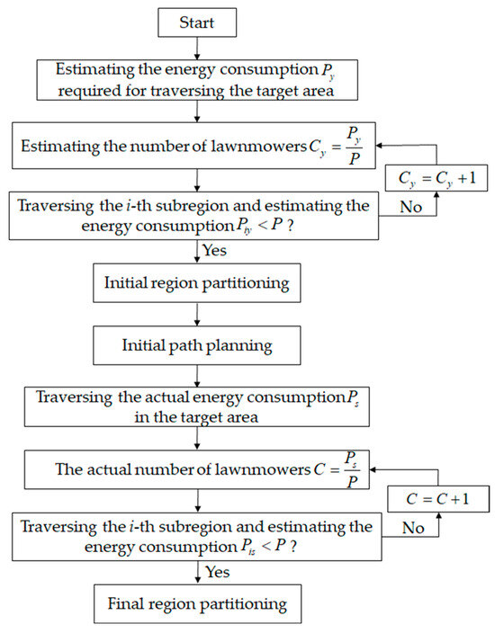
Figure 6.
Flowchart of the region partitioning process.
3.3. Task Assignment under Multiple Constraints
Multi-Robot Task Allocation (MRTA) for Multiple Robots is a critical issue for the functionality of multi-robot systems. It involves assigning tasks to each robot in a way that improves system efficiency. In the face of complex orchard terrain, individual lawnmowers may experience insufficient coverage due to their own carried energy limitations and the influence of intricate topography. This issue is addressed by creating logically constrained work zones and allocating segmented sub-regions to each lawnmower to ensure complete coverage of the target area. In a multi-robot system, the shortest working time is determined by the longest working time of a single robot. This section focuses on optimizing objectives such as reducing the working time of the cluster of lawnmowers and lowering the total cost. It considers the energy carried by each lawnmower and the energy consumption required for the work. The goal is to balance the working time of each lawnmower, aiming to enhance the overall efficiency of the lawnmower cluster while minimizing costs. This section discusses the task allocation problem for the lawnmower robot cluster from two perspectives: task allocation objectives and mathematical models for task allocation. When assigning tasks to the lawnmower robot cluster, the following principles are followed:
- (1)
- Rationality: This ensures that all the pending areas in the orchard are allocated to the corresponding lawnmower robots, guaranteeing the complete coverage of all pending areas in the orchard.
- (2)
- Minimization of travel distance: The goal is to minimize the travel distance for each lawnmower robot to reduce their energy consumption.
- (3)
- Fairness: Task allocation should be fair, ensuring that each lawnmower robot has an equal opportunity to perform tasks. (The principle of fairness employed in this study is instead integral as a strategic element for enhancing system efficiency. In this context, fairness refers to the equitable distribution of workloads among the robots, thereby optimizing the overall longevity and maintenance of the system. This approach ensures that no individual robot is subjected to continuous overload, which in turn mitigates the rate of wear and tear on each unit. Consequently, this strategy extends the operational lifespan of the entire fleet and maintains uniform performance levels across all units. Additionally, this principle enhances the system’s adaptability in dynamic operational environments. By ensuring a balanced task allocation, the system is better equipped to manage unforeseen changes, such as varying terrain challenges or individual robot malfunctions, thereby maintaining operational resilience and efficiency.)
The mathematical description of the cluster lawnmower task allocation problem is as follows: The simulated grid map of the orchard is divided into n pending areas based on the energy of the lawnmower robot itself. In the cluster lawnmower system, which consists of m lawnmower robots and n pending areas, the m lawnmower robots are represented by the set , and the n pending areas are represented by the set . Each pending area in the system only requires the allocation of one lawnmower robot to complete the task. A single lawnmower robot can only complete one task within a certain time period. However, after completing a task and receiving energy replenishment, the lawnmower robot can traverse and cover another area. The system’s objective is to allocate the n pending areas to the m lawnmower robots in a rational manner to improve work efficiency and minimize overall energy consumption.
Mathematical description of lawnmower task execution capability: The lawnmower’s ability to execute tasks refers to whether the lawnmower has the energy to perform a specific task. Let represent that lawnmower i can execute a task in target area j; likewise, indicates that lawnmower i cannot execute a task in target area j.
Energy consumption for individual lawnmower tasks: During the execution of a specific task, a lawnmower consumes a certain amount of energy, where the cost of an individual task is represented by a two-dimensional matrix D with dimensions . When a lawnmower moves from point a to point b, the distance between points a and b is . Therefore, the energy consumption for an individual task is .
Total energy cost incurred by the system (cost): Define a binary variable , where indicates whether the jth target coverage area has been assigned to the ith lawnmower . In this case, denotes that the jth target coverage area has not been assigned to the ith lawnmower . Given the task set for the ith lawnmower , which is , it represents that the ith lawnmower has been assigned to g target coverage areas, and the tasks are executed sequentially from to all the way to . Therefore, the energy cost incurred by the ith lawnmower in executing tasks in the assigned subareas is:
In a cluster lawnmower system comprising m lawnmowers and n target coverage areas, the total energy expenditure of the system is as follows:
From the above analysis, it is evident that the cluster lawnmower task allocation problem can be transformed into finding a suitable task allocation strategy and providing a set of target coverage areas for each lawnmower to minimize the total energy expenditure cost within the system. Additionally, the system must adhere to several constraint conditions to refine the specific task allocation. These specific constraint conditions include:
Constraint 1.
The constraint condition in Formula (15) signifies that each lawnmower can only traverse and cover a single subregion at a time, meaning that an individual lawnmower can only operate within its assigned task area.
Constraint 2.
The constraint condition in Formula (16) ensures that each pending coverage area is allocated a lawnmower to guarantee the coverage of all pending subregions.
Constraint 3.
The constraint condition in Formula (17) implies that the ith lawnmower is assigned to g pending subregions (in this study, each lawnmower corresponds to one pending coverage area, i.e., g = 1).
Constraint 4.
The constraint condition in Formula (18) implies that the lawnmower with the ith identifier has the capability to execute g pending subregions (g = 1) with the energy it carries.
3.4. Improved A* Algorithm and Experimental Verification
3.4.1. Improved A* Algorithm
Common path planning algorithms, such as Dijkstra’s algorithm, ensure the discovery of the shortest path from the starting point to the destination. However, it employs a greedy strategy, which makes it incapable of handling graphs with negative-weight edges, as these edges can result in incorrect shortest paths. Furthermore, the search speed is relatively slow due to the large number of explored nodes. Although the traditional A* algorithm is effective in path planning, it often expands numerous nodes during the search process, leading to a significant accumulation of turning angles. Therefore, this paper proposes an improved A* algorithm by weighting the heuristic cost function and introducing a turning cost into the total cost function. An eight-neighbor expansion method for pathfinding is employed based on the actual working conditions of the lawnmower. This improvement aims to enhance the search speed of the algorithm, increase the optimality of the global path, and reduce the number of turns made by the robot during traversal, thereby shortening the overall travel time.
Firstly, this study employs the Manhattan distance as the heuristic function, which calculates the sum of the distances along the x-axis and the y-axis between the current point and the target point as the heuristic cost function’s value.
where refers to the coordinates of the target point, whereas corresponds to the coordinates of the current point.
In the actual search process, as the estimated cost function h(n) cannot be known in advance, it is assumed that the estimated distance from the current node n to the goal node is represented by H(n). When replacing h(n) with H(n) in the A* algorithm, the actual shortest path in the A* algorithm must always be greater than or equal to the value of the heuristic function h(n), i.e., h(n) ≥ H(n). If h(n) > H(n), the efficiency of the A* algorithm is slightly reduced and it cannot guarantee the optimal path will be found, but it does maintain high accuracy. If h(n) = H(n), the A* algorithm strictly follows the shortest path during the search, ensuring the optimal path while reducing the expansion of nodes, significantly improving efficiency. However, this scenario is not suitable when obstacles are present in the environment. If h(n) < H(n), the A* algorithm expands more nodes in the search, but it ensures the optimal path will be found. Since the orchard environment has certain obstacles, when the Manhattan distance is applied in environments with obstacles, its estimated cost function h(n) is often less than the estimated distance H(n) from the current point to the target point. To address this issue, this paper introduces a weighting mechanism to the A* algorithm’s estimated cost function h(n). This involves multiplying by a coefficient k (k > 1), resulting in the modified overall cost function expression:
where g(n) represents the current cost from the starting point to the current node.
The choice of the constant k is based on balancing two distance estimates to ensure that the influence of the Manhattan distance is not overly significant when considering obstacles. Selecting an appropriate value for k requires experimentation and testing. In the MATLAB platform, a grid map size of 20 × 20 is set with an arbitrary distance l of 2 between any two adjacent grid cells. Through calculations, the weighted value k in the heuristic cost function is chosen as 1.3 to achieve a balanced point for obtaining the optimal path. At this point, the value of the weighted heuristic cost function from the current node to the target node tends to infinity, approaching the estimated distance from the current node to the target node. This modification aims to reduce the expansion of nodes in the A* algorithm, thereby improving search speed and yielding an improved A* path.
Secondly, to reduce the issue of the lawnmower making frequent turns during actual movement, this paper introduces a turning cost to the current cost function . Additionally, on top of the weighted heuristic cost function , a turning cost is also added to the term . Therefore, when calculating the current cost , the following steps should be followed (here, refers to the cost from the current node n to the node to be expanded ):
- (1)
- Check if the current node n is the initial node, i.e., if there is a parent node m that precedes the current node.
- (2)
- If the current node n is the initial node, meaning there is no parent node m for the current node n, then use the coordinates of the current node n and the coordinates of the node to be expanded, denoted as r, to calculate the turning cost. When , indicating that the current node n and the node to be expanded r are not on a horizontal or vertical line, and the node r is in the left-up, left-down, right-up, or right-down direction from the current node, the current cost function from the current node n to the node to be expanded r is expressed as:where l represents the distance between two adjacent nodes in the horizontal or vertical direction. When , indicating that the current node n and the node to be expanded r are aligned in the horizontal or vertical direction, the current cost function from the current node n to the node to be expanded r is expressed as:
- (3)
- If the current node n is not the initial node, meaning that the current node n has a parent node m, then the cost of turning is determined using the coordinates of the current node n and its parent node m . When , indicating that the current node n and the parent node m are not collinear in the horizontal or vertical direction, the current cost function from the parent node m to the current node n is expressed as ; when , meaning that the parent node m and the current node n are collinear in the horizontal or vertical direction, the current cost function is expressed as . After these improvements, the overall cost function is , where is calculated using the formula or depending on different situations.
3.4.2. Experiments and Conclusions
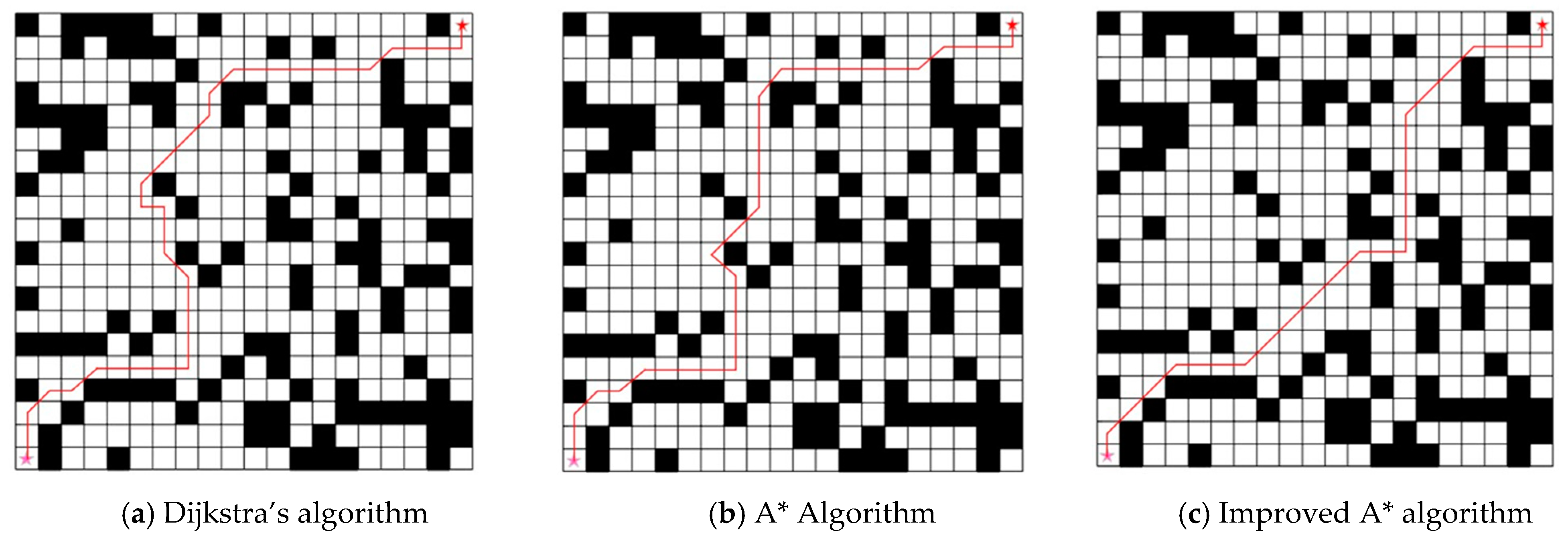
In this section, the improved A* algorithm was simulated and experimentally validated on a platform with 8 GB of computer memory, a processor frequency of 3.2 GHz, and based on MATLAB 2020b. Comparative analyses were conducted among the traditional A* algorithm, Dijkstra’s algorithm, and the improved A* algorithm proposed in this section in different application scenarios. The grid map was set to a size of 20 × 20, with the distance between any adjacent two grid cells defined as l = 2. After calculation, the weighted factor k in the heuristic cost function was selected as 1.3. The algorithm’s iteration count was set to 400 times. Twenty-five percent of the grid cells in the map were designated as obstacle cells, and the positions of these obstacles were randomly distributed on the grid map. The starting point of the lawnmower robot was set to [1,1], and the target endpoint was set to [20,20]. The simulation results are shown in Figure 7. The comparison of path length, turn counts, and search time of the three algorithms is shown in Table 1.
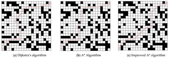
Figure 7.
Dijkstra’s algorithm, A* algorithm, and improved A* algorithm search path simulation. (White grids represent grids where the lawnmower can travel, black grids indicate obstacle grids and the red lines are the optimal paths generated by the different algorithms).

Table 1.
Comparison of path length, turn counts, and search time.
From Table 1, it can be concluded that the improved A* algorithm had fewer turns, a shorter path for robot travel, and a more superior planned path compared to the first two algorithms. This advantage was more pronounced in areas with many obstacles.
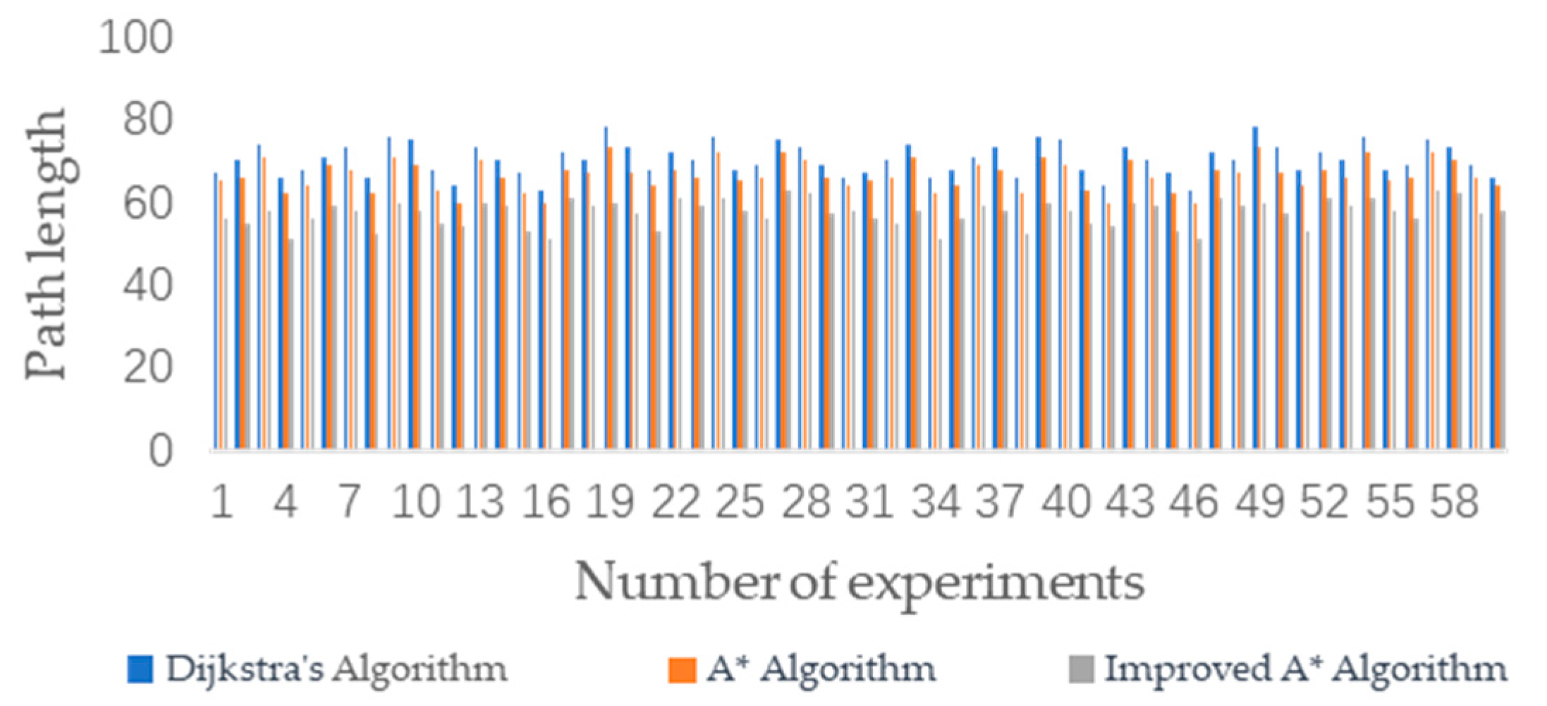
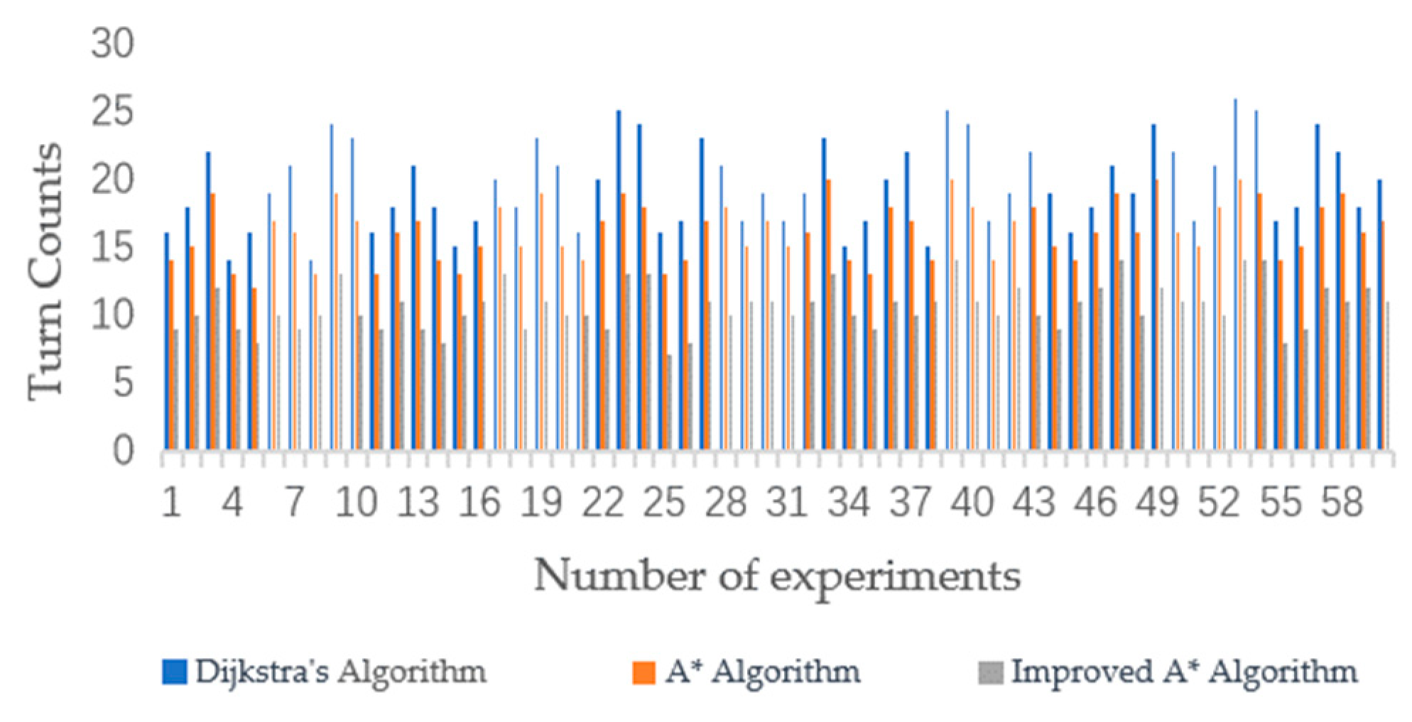
The three algorithms were subjected to 60 simulation experiments on different grid maps. The experimental results are shown in Figure 8 and Figure 9. Through multiple experiments, the improved A* algorithm proposed in this study demonstrated superior performance in terms of the number of turns and the length of the path compared to the other two algorithms.
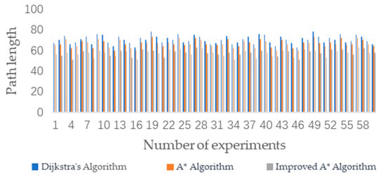
Figure 8.
Comparison of path lengths among the A* algorithm, Dijkstra’s algorithm, and the improved A* algorithm.

Figure 9.
Comparison of turn counts between the A* algorithm, Dijkstra’s algorithm, and the improved A* algorithm.
The average path length and turn counts for the three algorithms in these 60 simulation experiments are shown in Table 2.

Table 2.
Comparison of average path length, turn counts, and search time.
From Table 2, it can be observed that in terms of the average path length, the A* algorithm was close to the Dijkstra algorithm. The average path length for the improved A* algorithm was 57.61, whereas for the traditional A* algorithm, it was 66.53, representing a reduction of approximately 13.4%. In terms of average turning times, the traditional A* algorithm had 14.22 turns, whereas the improved A* algorithm had 12.36 turns, a reduction of approximately 13.1%. Additionally, the average search time for the improved A* algorithm was reduced by 14.19%. The data indicate that the improved A* algorithm exhibited superior performance relative to its predecessor due to its enhanced heuristic approach and the incorporation of turning cost analysis into its cost function. The algorithm’s heuristic functions are weighted to prioritize paths that seem more efficient, thereby reducing the search for suboptimal paths. This approach speeds up the pathfinding process and leads to shorter path lengths. Concurrently, incorporating turning cost considerations into the algorithm’s cost function promotes the identification of more linear and direct routes, reduces the number of turn counts, and optimizes both path length and computational efficiency. The experimental results strongly suggest that the benefits of these algorithmic improvements in terms of path length and number of turn counts clearly outweigh the potential limitations of the algorithm, such as increased computational complexity and reduced applicability.
4. Path Planning Simulation and Field Experiment Verification with Different Numbers of Clustered Lawnmowers
4.1. Evaluation Metrics for Lawnmower Full-Coverage Path Planning
In the process of traversing the orchard, the lawnmower needs to cover the entire orchard at the smallest possible cost. Therefore, this section proposes quantitative evaluation metrics to assess the performance of the algorithm. In this study, the full-coverage path planning algorithm is based on a grid map, and it is assumed that the total number of grid cells in the simulated environment map is , where represents the number of grid cells occupied by obstacles, represents the number of grid cells missed by the lawnmower, represents the number of grid cells revisited by the lawnmower, represents the total energy consumption of the lawnmower while traversing the orchard, represents the total number of lawnmowers, and represents the total cost of the lawnmowers traversing the orchard.
- (1)
- Repetition rate: Upon completing the orchard traversal, the percentage of all repeated grid cell occurrences to the total number of grid cells, excluding obstacles, is determined.
- (2)
- Omission rate: Upon completing the orchard traversal, the percentage of all missed grid cell occurrences to the total number of grid cells, excluding obstacles, is determined.
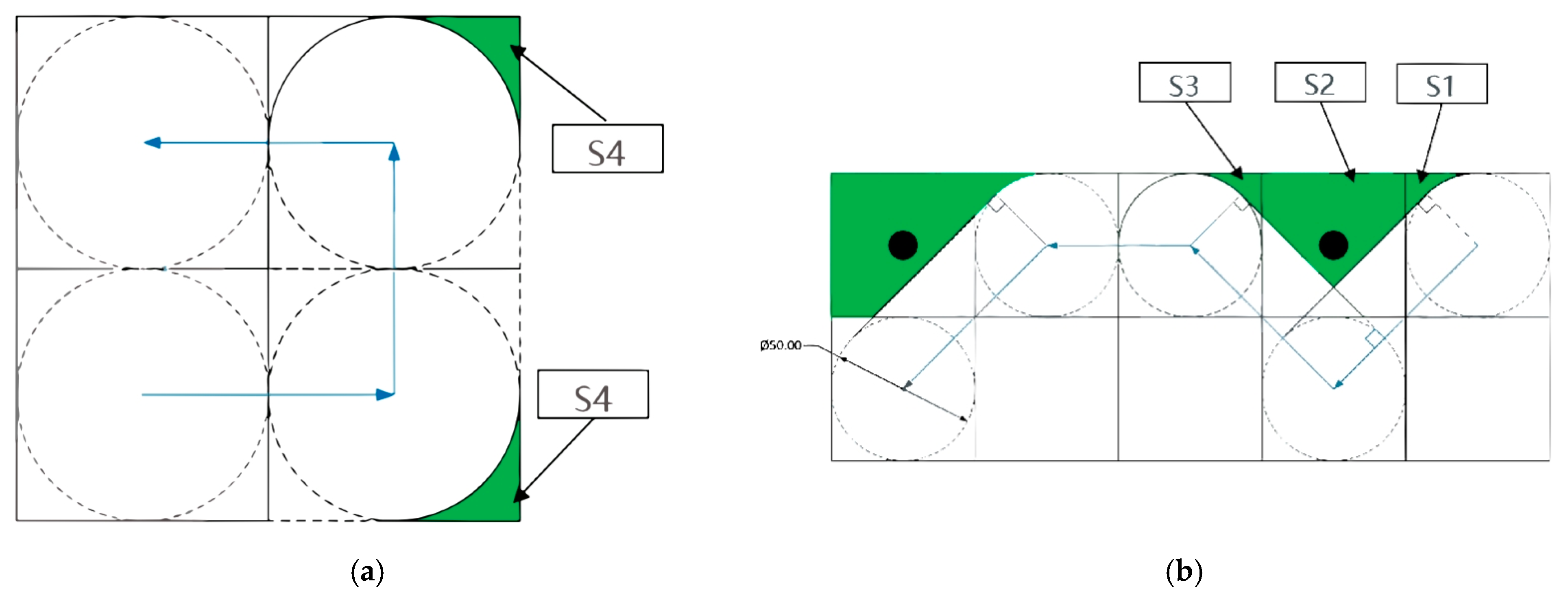
In this study, the omission rate of the lawnmower during its travel process mainly includes two types: The first type is the missed coverage during right-angle turns, and the second type is the missed coverage when the lawnmower circumvents fruit trees. These two types of missed mowing areas are shown in Figure 10.
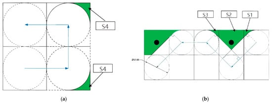
Figure 10.
The area of missed mowing. (a) The missed mowing areas during right-angle turns. (b) The missed mowing areas when circumventing fruit trees. (, , , are missing cut regions).
- (3)
- Total cost: This refers to the sum of the fuel consumption of the lawnmower and the cost of the lawnmower itself after the lawnmower completes its traversal of the orchard.
4.2. Connected Orchard Coverage Path Planning
The grid map was set to a size of 40 × 40, and the distance between any two adjacent grid cells was denoted as l = 0.6 m. The obstacle occupancy rate (the ratio of the number of grid cells occupied by obstacles to the total number of grid cells) was o = 6%, with fruit trees denoted as fixed obstacles on the grid map. The grid map was divided into the following regions: White cells represent areas accessible by the lawnmower, indicating regions where the lawnmower can achieve the highest travel speed during operation, with a total of cells. Black cells represent obstacles, i.e., impassable cells. Pink cells represent uphill areas, with a total of cells. Blue cells represent downhill areas, with a total of cells. Red cells represent areas with dense weeds, with a total of cells. Yellow cells represent areas with sparse weeds, which have a negligible impact on the operation of the lawnmowers. The simulated grid map created based on Section 2 is shown in Figure 11.
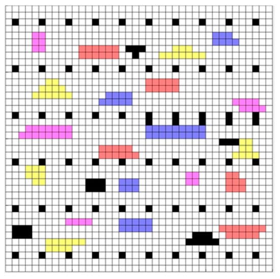
Figure 11.
Grid map of the connected orchard. (White grids represent grids where the lawnmower can travel, gray grids indicate obstacle grids (i.e., impassable grids), pink grids represent uphill areas, blue grids denote down-hill areas, red grids represent overgrown grass areas, and yellow grids represent areas with sparse weeds).
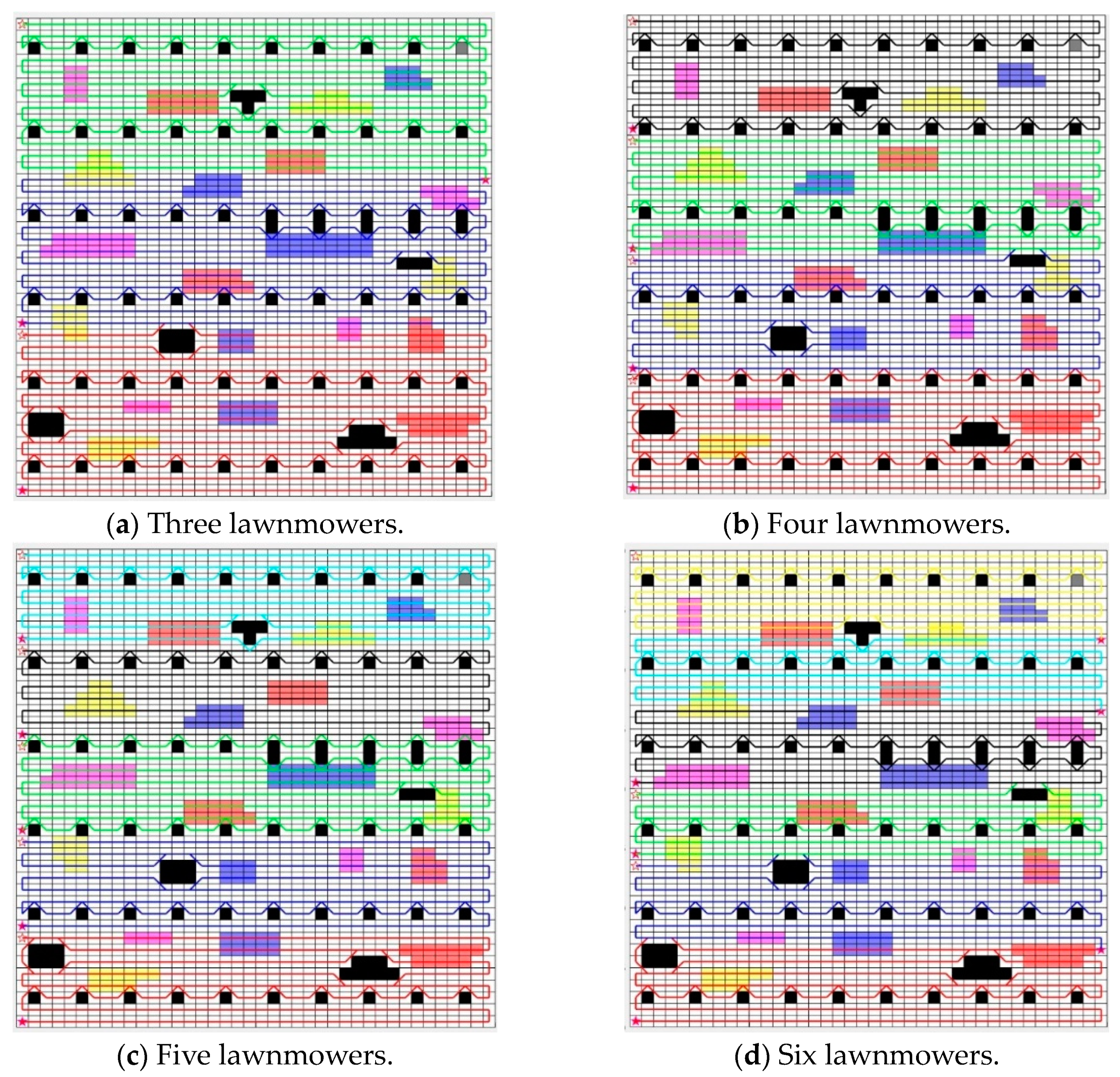
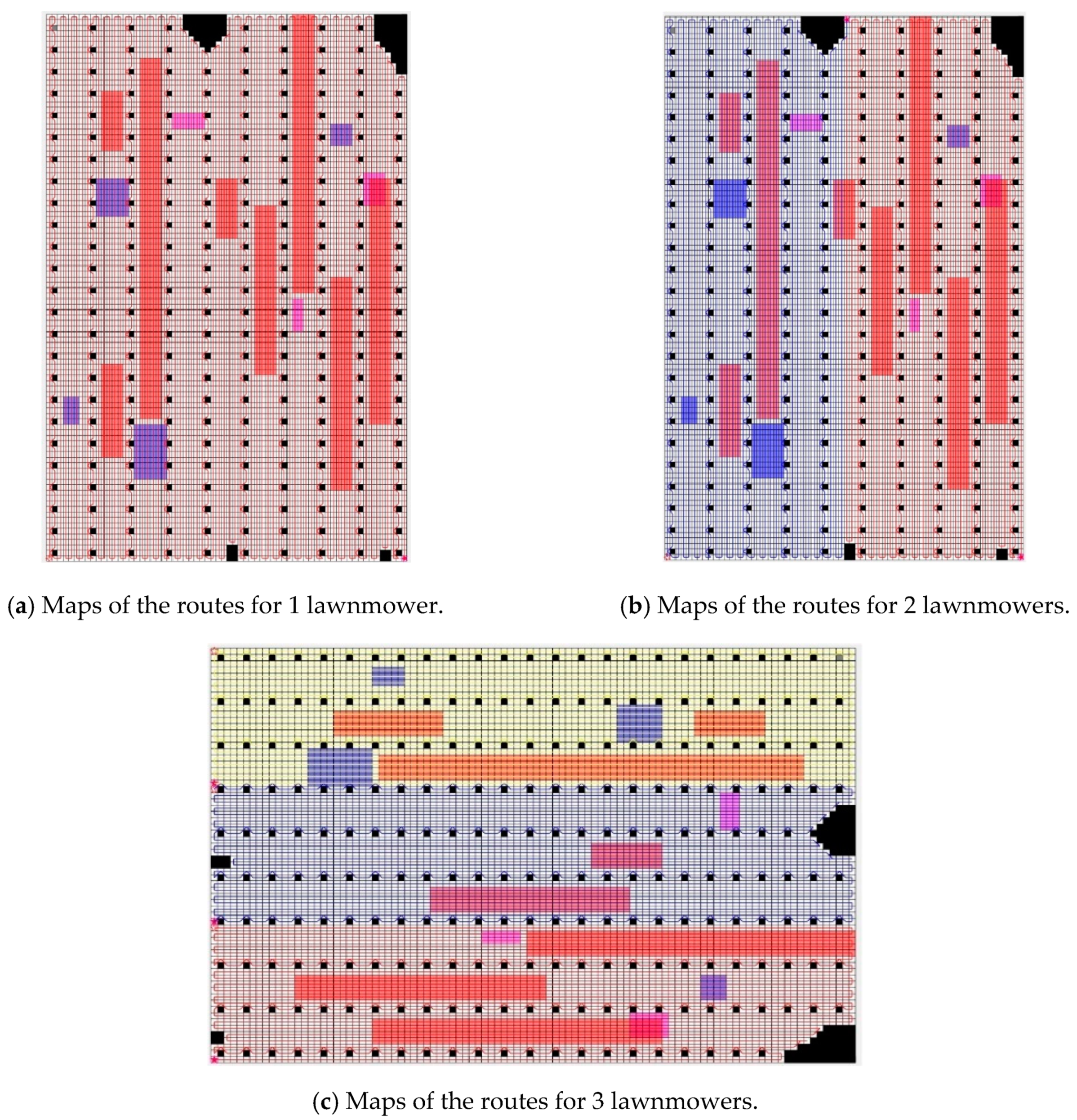
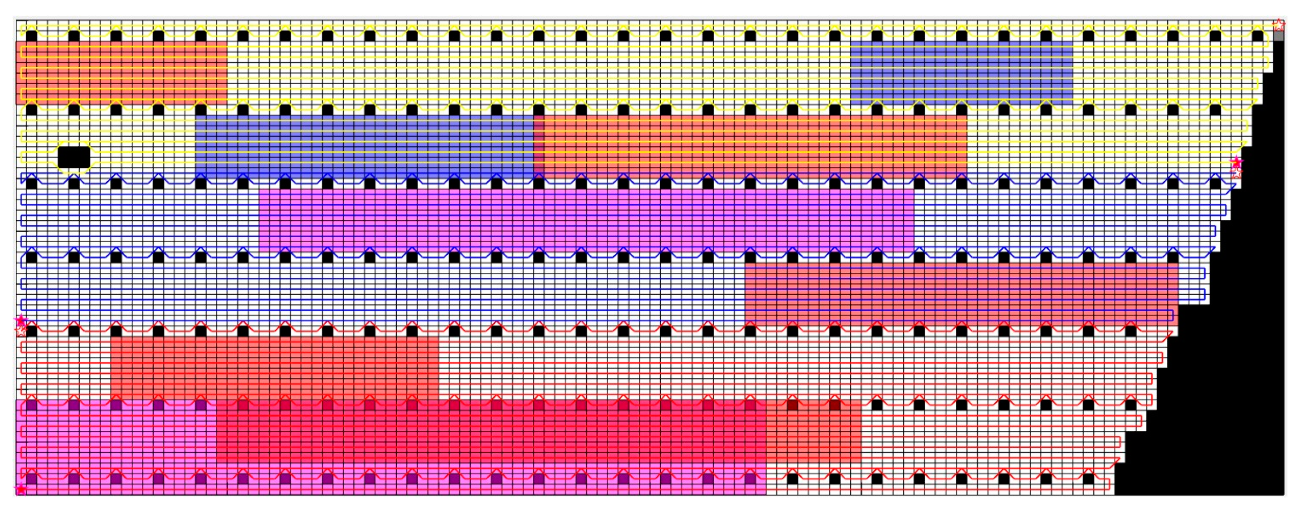
The improved A* algorithm was defined with the following parameters: The weighted value in the heuristic function was chosen as k = 1.3, and the maximum number of iterations was set to 500. The coordinates of the initial position of the lawnmower robot were set at [1,1], and the endpoint was determined by the optimization goal. Each lawnmower carried an energy capacity of p = 28,800 kJ. The normal speed of the lawnmower when traveling in each white grid cell was v = 1.5 m/s, with an energy consumption rate of . In the uphill region (pink grids), the speed constraint coefficient was set to . For downhill regions (blue grids), the constraint coefficient was . In areas with dense weeds (red grids), the constraint coefficient was . As shown in Figure 12, different colors represent the paths of different lawnmowers. When the number of lawnmowers significantly exceeds the minimum required for complete coverage of the grid map, it is essential to determine the initial minimum number of lawnmowers. This is accomplished by using a formula to estimate the minimum number of lawnmowers required for the grid map.
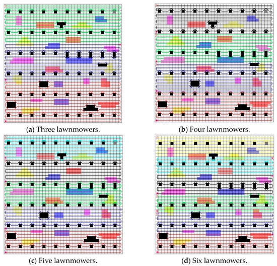
Figure 12.
The travel route maps for 3, 4, 5, and 6 lawnmowers in the connected orchard. (White grids represent grids where the lawnmower can travel, gray grids indicate obstacle grids (i.e., impassable grids), pink grids represent uphill areas, blue grids denote down-hill areas, red grids represent overgrown grass areas, and yellow grids represent areas with sparse weeds. The lines in the picture show the routes of the robots).
To evaluate the impact of different numbers of lawnmowers on path planning, four sets of experiments were conducted for path planning in the connected orchard. In the first set of experiments, the number of lawnmowers was set to three; in the second set, it was set to four; in the third set, it was set to five, and in the fourth set, it was set to six. This simulation experiment evaluated the influence of different numbers of lawnmowers on path planning under identical grid map conditions. The simulation was performed on a computer with 8 GB of memory and an AMD R7-5800 CPU, using MATLAB 2020b as the simulation software.
Therefore, this simulation experiment compared cases where the number of lawnmowers was set to three, four, five, and six, analyzing the repetition rate, omission rate, energy consumption, and cost of the lawnmowers. The improved A* path for each lawnmower in scenarios with different numbers of lawnmowers is shown in Figure 12 below.
In this simulation experiment, lawnmower travel directions were determined based on Figure 5. The total operation time, individual lawnmower working time, total energy consumption, and energy consumption per lawnmower for configurations with three, four, five, and six lawnmowers are summarized in Table 3.

Table 3.
Comparison of lawnmower working time, energy consumption, and cost in the connected orchard.
For this simulation experiment, the repetition rate and omission rate of the grid map traversal for three, four, five, and six lawnmowers are summarized in the Table 4.

Table 4.
The experimental results for the lawnmower robot omission rate and repetition rate in the connected orchard.
From Table 3 and Table 4, it can be observed that, with a constant grid map, as the number of lawnmower clusters increased, the minimum working time of lawnmowers in this grid map gradually decreased. However, the decreasing trend of the minimum working time diminished with the increasing number of lawnmowers. In terms of omission rate, as the number of lawnmower clusters increased from three to six, the omission rate gradually decreased. Similarly, the decreasing trend continued with the increasing number of lawnmower clusters. Regarding the repetition rate, when the number of lawnmowers increased from three to five, the repetition rate decreased. However, when the number of lawnmowers increased from five to six, the repetition rate increased by 0.30%. Simultaneously, with an increase in the number of lawnmowers, the total working cost of the lawnmowers increased. Therefore, in this simulation experiment, when the lowest repetition rate and omission rate of lawnmowers were considered as evaluation indicators, the optimal number of lawnmower clusters was five.
4.3. Covering Path Planning in Non-Connected Orchards
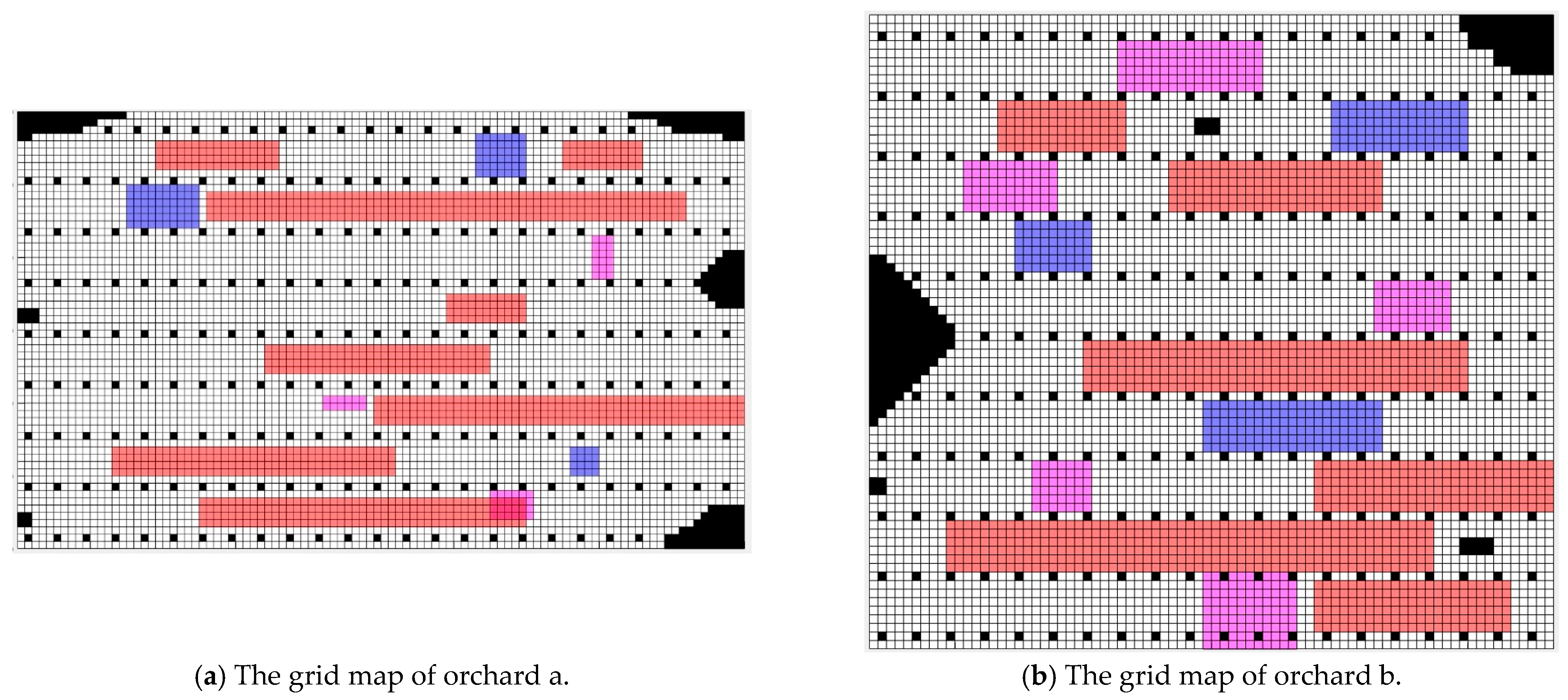
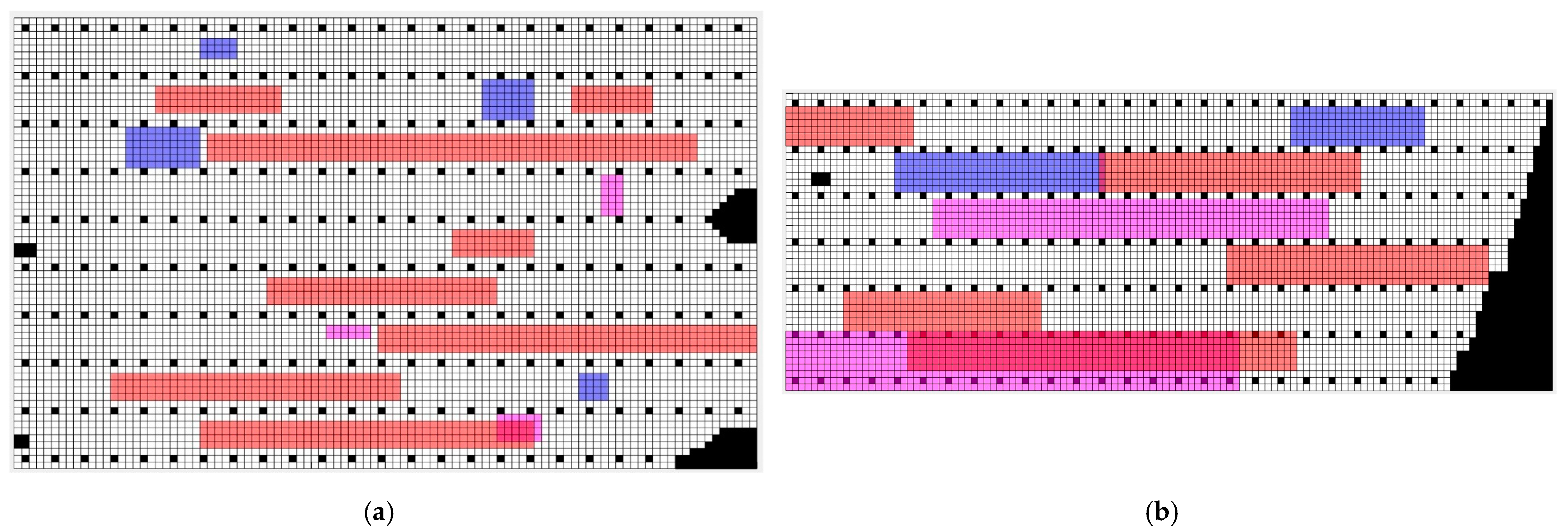
For the non-connected orchards, the following definitions were established. The orchards were denoted as two independent entities (labeled a and b). The size of the grid map for orchard a was set to 100 × 60, and for orchard b, it was set to 80 × 74. The obstacle occupancy rate in the grid map for orchard a (the ratio of the number of grid cells occupied by tree obstacles to the total number of grid cells) was o = 6.55%, and for orchard b, it was 6.93%. The distance between any two adjacent grid cells was denoted as l = 50. The grid map was categorized into the following regions: White cells represent areas where the lawnmower can move, achieving its maximum speed in operational conditions; black cells represent obstacles, indicating impassable areas; pink cells represent uphill regions, with the total number of uphill cells being for orchard a and for orchard b; blue cells represent downhill regions, with cells for orchard a and cells for orchard b; and red cells represent areas with dense grass, with cells for orchard a and cells for orchard b. The grid maps for the non-connected orchards are illustrated in Figure 13.
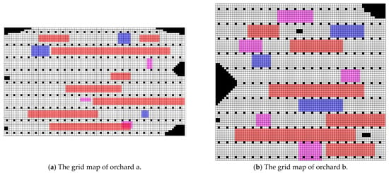
Figure 13.
The grid map of the non-connected orchards. (White grids represent grids where the lawnmower can travel, gray grids indicate obstacle grids (i.e., impassable grids), pink grids represent uphill areas, blue grids denote down-hill areas, red grids represent overgrown grass areas).
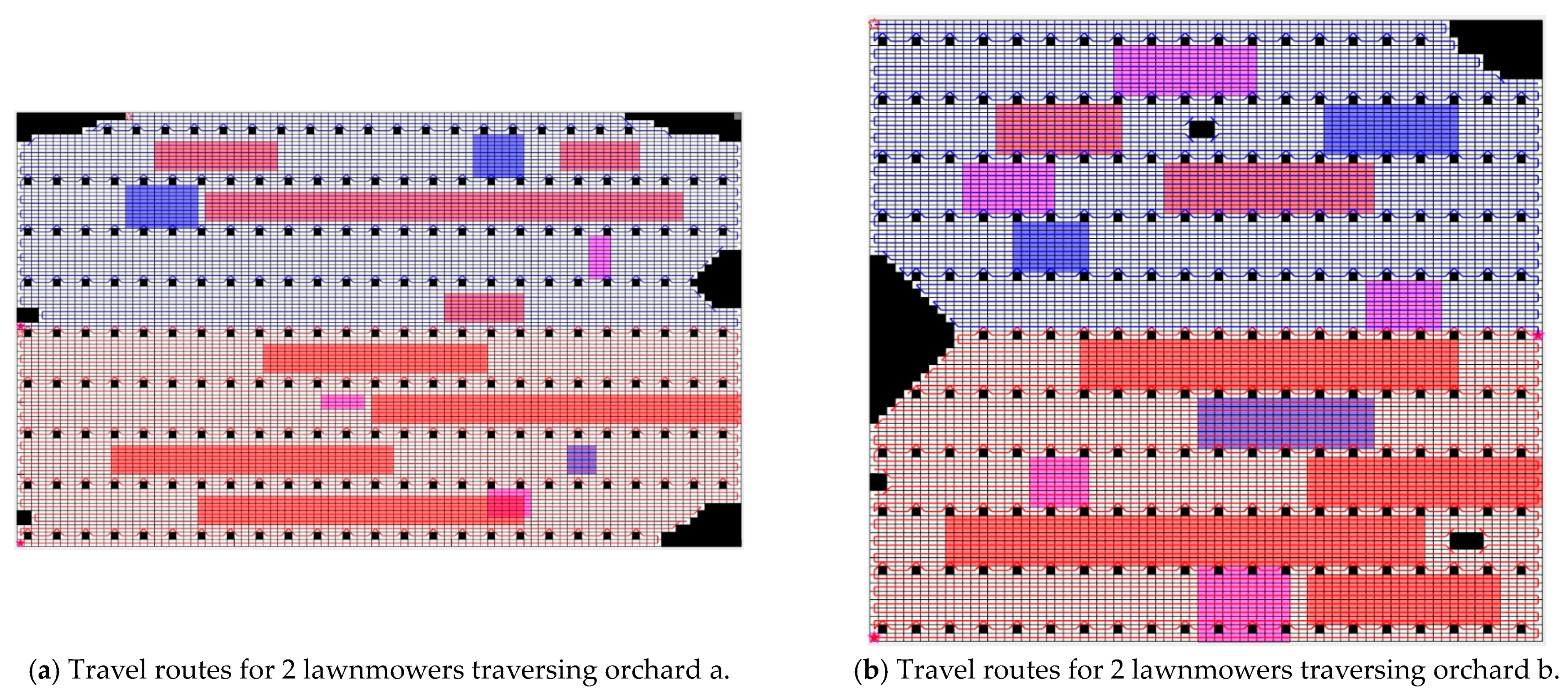
To validate the impact of different numbers of lawnmowers on path planning, experiments were conducted on the non-connected orchards. Prior to these experiments, the minimum number of lawnmowers required to traverse and cover orchard a was determined to be two, and for orchard b, it was also determined to be two. Therefore, for this simulation experiment, four and five lawnmowers were set up, and four sets of experiments were conducted.
In the first set of experiments, the four lawnmowers were divided into two clusters, each containing two lawnmowers. Both clusters of lawnmowers simultaneously traversed orchards a and b. The experiment recorded the lawnmowers’ shortest working time, repetition rate, omission rate, and cost during the traversal process. The improved A* paths for each lawnmower are shown in Figure 14.
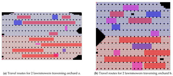
Figure 14.
Travel route maps for the lawnmowers in Experiment 1. (White grids represent grids where the lawnmower can travel, gray grids indicate obstacle grids (i.e., impassable grids), pink grids represent uphill areas, blue grids denote down-hill areas, red grids represent overgrown grass areas. The lines in the picture show the routes of the robots).
The data for the lawnmowers in Experiment 1 during the traversal of orchards a and b in terms of time, energy consumption, and cost are recorded in Table 5.

Table 5.
The data for time, energy consumption, and cost in Experiment 1.
The data for the repetition rate and the omission rate of the lawnmower during the traversal of grid maps for orchards a and b in the first set of simulation experiments are recorded in Table 6.

Table 6.
Experimental results for repetition rate and omission rate in Experiment 1.
From Table 5 and Table 6, it can be observed that in the first set of simulation experiments, the shortest working time for traversing and covering orchard a was 2098.21 s, and for orchard b, it was 2060.47 s. Since the two groups of lawnmowers simultaneously traversed and covered orchards a and b, the shortest time for traversing and covering the non-connected orchards was 2098.21 s. As shown in the table, the repetition rate of lawnmower traversal and coverage for orchard a was 4.12%, and for orchard b, it was 4.25%. The total repetition rate for non-connected orchards was calculated using the following formula:
The repetition rate for the non-connected orchard was 4.18%. The mowing machine’s traversal coverage omission rate for orchard a was 0.24%, and for orchard b, it was 0.19%. The total omission rate for non-connected orchards was calculated using the following formula:
The total omission rate for the non-connected orchards was 0.21%.
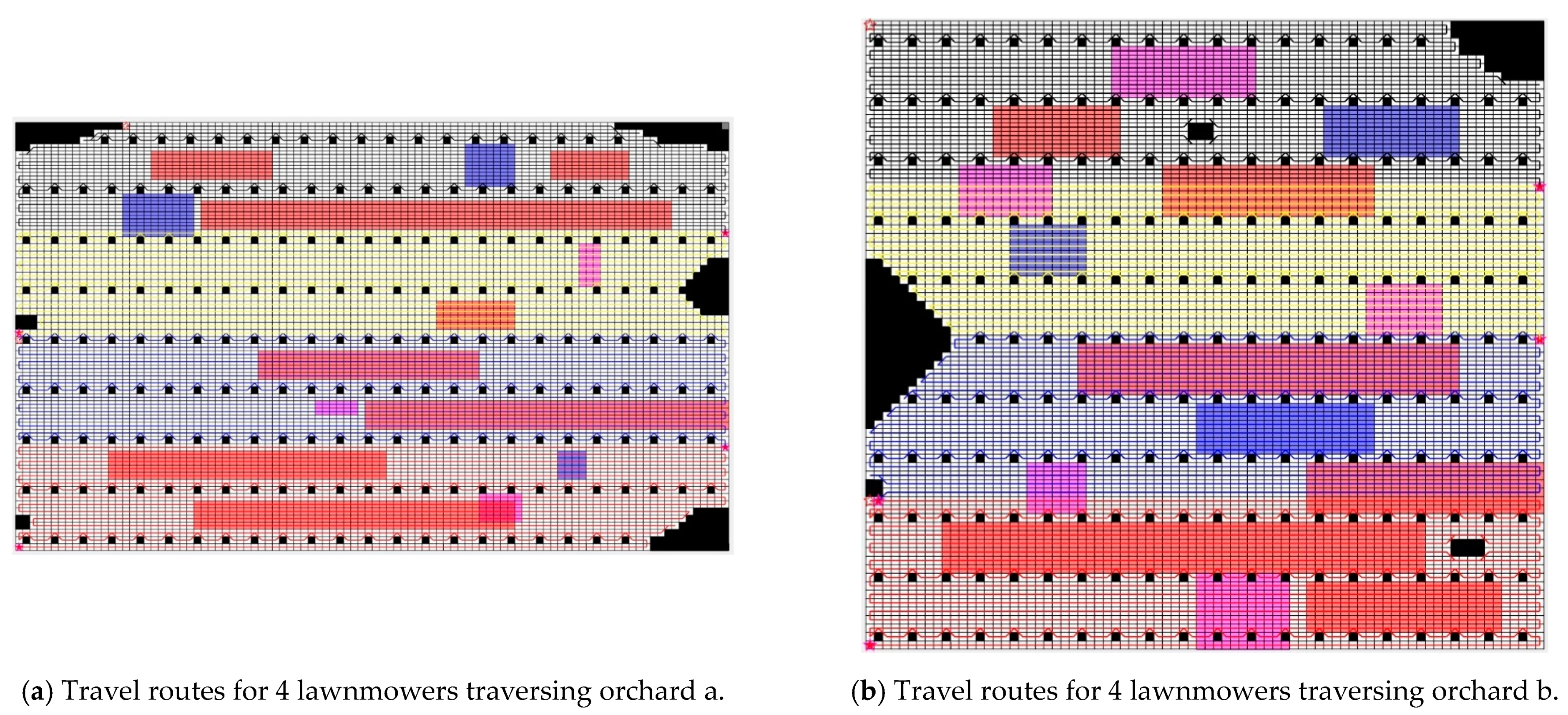
Experiment 2 involved grouping the four lawnmowers together, resulting in a cluster count of four. The lawnmowers in this group sequentially traversed orchards a and b. After completing the first orchard, they required an energy refill, with the assumed refueling time being 300 s. The recorded data include the lawnmowers’ minimum working time, repetition rate, omission rate, and cost during the traversal process. The improved A* paths for each lawnmower are depicted in Figure 15.
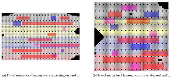
Figure 15.
Travel route maps for the lawnmowers in Experiment 2. (White grids represent grids where the lawnmower can travel, gray grids indicate obstacle grids (i.e., impassable grids), pink grids represent uphill areas, blue grids denote down-hill areas, red grids represent overgrown grass areas, and yellow grids represent areas with sparse weeds. The lines in the picture show the routes of the robots).
The data for the lawnmowers in Experiment 2 during the traversal of orchards a and b in terms of time, energy consumption, and cost are recorded in Table 7.

Table 7.
The data for time, energy consumption, and cost in Experiment 2.
The data for the lawnmowers in Experiment 2 during the traversal of orchards a and b in terms of repetition rate and omission rate are recorded in Table 8.

Table 8.
Experimental results for repetition rate and omission rate in Experiment 2.
From Table 7 and Table 8, it can be observed that in the second set of simulation experiments, the shortest working time for traversing and covering orchard a was 1058.30 s, and for orchard b, it was 1039.78 s. Since the two groups of lawnmowers traversed and covered orchards a and b sequentially, and energy replenishment was required after completing the traversal and coverage of the first orchard, the shortest time for the lawnmowers to traverse and cover the non-connected orchards in Experiment 2 was 2098.07 s. According to Table 7, the repetition rate of the lawnmowers for orchard a was 4.16% and for orchard b it was 4.27%, and the total repetition rate for non-connected orchards was calculated using Formula (30) to be 4.21%. The omission rate of the lawnmowers for orchard a was 0.24% and for orchard b it was 0.19%, and the total omission rate for non-connected orchards was calculated using Formula (31) to be 0.21%.
Comparing the data from the first and second sets of experiments, for non-connected orchards, when the number of lawnmowers was constant, dividing the lawnmowers into two groups resulted in a shorter shortest working time of 2060.47 s compared to 2098.07 s when the lawnmowers were in one group. Furthermore, dividing the lawnmowers into two groups led to a lower repetition rate than having them in one group, whereas the omission rate shows little variation.
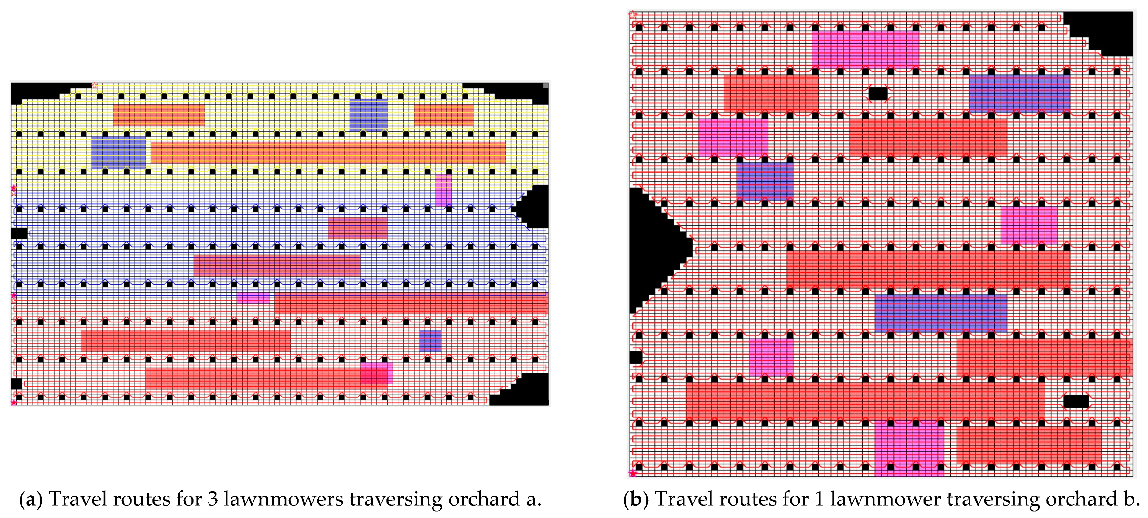
Experiment 3 involved dividing the four lawnmowers into two groups, with one lawnmower in one group and three lawnmowers in the other. The lawnmower cluster with a size of three traversed the larger area of orchard a, whereas the cluster with a size of one covered the smaller area of orchard b. Both groups of lawnmowers simultaneously traversed orchards a and b, and the experiment recorded the lawnmowers’ shortest working time, repetition rate, omission rate, and cost during the traversal process. The improved A* paths for each lawnmower are illustrated in Figure 16.
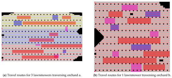
Figure 16.
Travel route maps for the lawnmowers in experiment 3. (White grids represent grids where the lawnmower can travel, gray grids indicate obstacle grids (i.e., impassable grids), pink grids represent uphill areas, blue grids denote down-hill areas, red grids represent overgrown grass areas, and yellow grids represent areas with sparse weeds. The lines in the picture show the routes of the robots).
The data for the lawnmowers in experiment 3 during the traversal of orchards a and b in terms of time, energy consumption, and cost are recorded in Table 9.

Table 9.
The data for time, energy consumption, and cost in experiment 3.
The data for the lawnmowers in experiment 3 during the traversal of orchards a and b in terms of repetition rate and omission rate are recorded in Table 10.

Table 10.
Experimental results for repetition rate and omission rate in experiment 3.
From Table 9 and Table 10, it can be observed that in the third set of simulation experiments, the shortest working time for traversing and covering orchard a was 1399.76 s and for orchard b it was 4103.29 s. Since the two groups of lawnmowers simultaneously traversed and covered orchards a and b, the shortest traversal time for the non-connected orchards was 4103.29 s. According to Table 9, the repetition rate of lawnmower traversal coverage for orchard a was 4.12% and for orchard b it was 4.23%. Using Formula (30), the total repetition rate for non-connected orchards was determined to be 4.17%. The omission rate of lawnmower traversal coverage for orchard a was 0.24% and for orchard b it was 0.19%. Using Formula (31), the total omission rate for non-connected orchards was determined to be 0.21%.
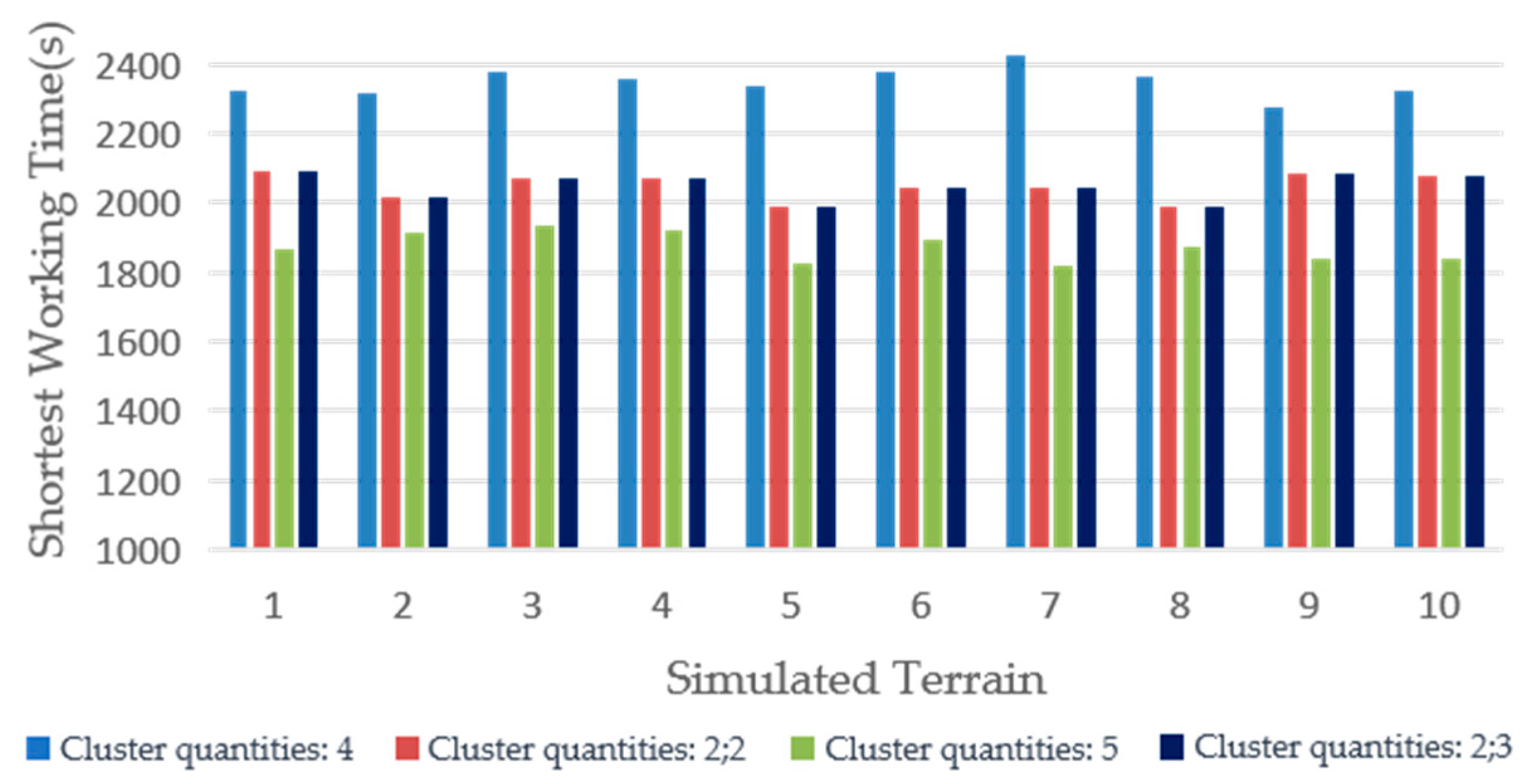
Comparing the results of the experiments in groups 1, 2, and 3, it was observed that dividing the lawnmower cluster into smaller clusters, especially when the cluster number could be evenly distributed, yielded better performance in terms of the shortest working time, repetition rate, and omission rate compared to treating the lawnmowers as a single collective cluster. This improvement was particularly evident in the case of the shortest working time. However, when the cluster number could not be evenly distributed, the performance in terms of the shortest working time, repetition rate, and omission rate was worse compared to treating the lawnmowers as a single collective cluster, with significant differences in the shortest working time. To validate this conclusion, 10 sets of simulation experiments were conducted on different non-connected orchards. For each non-connected orchard, four and five lawnmowers were selected for verification. The simulation experiments were conducted with four lawnmowers grouped according to the grouping in the first and second experiments and five lawnmowers grouped according to the grouping in the second and third experiments. The simulation results are shown in Figure 17.
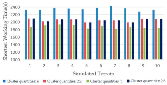
Figure 17.
Shortest working time simulation experiment data.
Therefore, for non-connected orchards, when the number of lawnmowers was fixed, the most optimal working effect was achieved by evenly distributing the number of lawnmowers in a cluster according to the number of components in the non-connected orchard. When the number of lawnmowers in a cluster could not be evenly distributed according to the number of components in the non-connected orchard, the optimal working effect was achieved by treating the lawnmowers as a single group.
4.4. On-Site Experiment Validation
In the actual orchard environment, due to the differences between the real operating conditions of the lawnmower and the simulated operating conditions of the lawnmower, there were discrepancies between the results of the simulation experiments and the actual experiments. Therefore, to validate the rationality of the path planning algorithm, field experiments were designed for research and analysis.
4.4.1. Selection of Experimental Site and Equipment
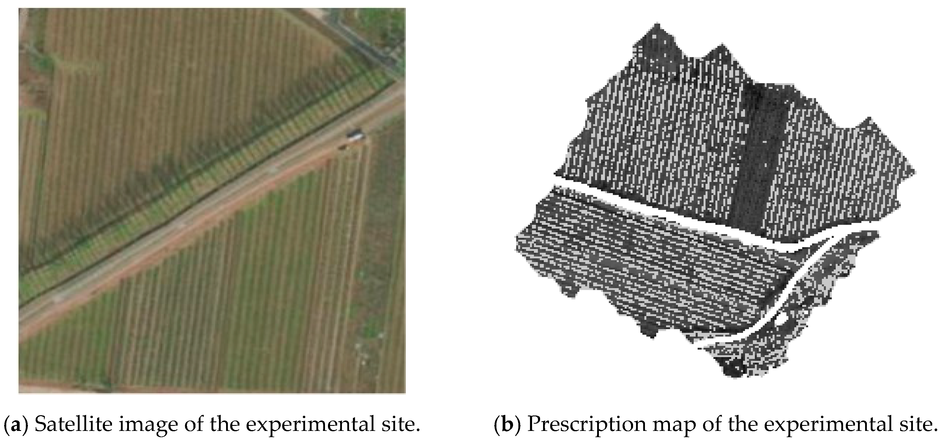
To better align the simulation conditions of the lawnmower with its actual working environment, the selected orchard had a terrain slope ranging from 0 to 10 degrees, meeting the experimental requirements. The satellite image of the orchard is shown in Figure 18a, and the prescription map of the orchard based on Section 2 is shown in Figure 18b. The basic data of the experimental site are presented in Table 11.
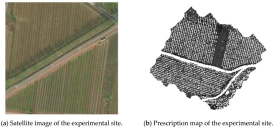
Figure 18.
Satellite image and prescription map of the experimental site.

Table 11.
The basic data of the experimental site.
The basic data of the experimental site are presented in Table 11.
The robotic lawnmower used in the experiment was designed and assembled by our team. Its main operating principle is as follows: The locomotion system is independently powered by a 48 V DC power supply. It employs a tracked dual-motor driving mechanism, providing stable movement and obstacle-crossing capabilities in hilly orchard terrains. The differential rotation of the dual motors enables the lawnmower to achieve minimum radius turns. The cutting system is powered by a gasoline engine with a rated speed of 3600 rpm. The power is transmitted from the engine’s output shaft, passing through a first-stage gear reducer for appropriate speed reduction before being transmitted to the blade disc output shaft. This, in turn, drives the rapid rotational cutting motion of the blade disc and the blades. The lifting mechanism primarily consists of a parallelogram mechanism and an electric push rod. The platform, linkages, and linkages with the frame adopt articulated connections to ensure relative motion space. The telescopic movement of the electric push rod is converted into the platform’s upward and downward motion, facilitating weed removal for different ground conditions and cutting heights. Additionally, the engine employed in the lawnmower robot for the experiments is a dedicated power source for the cutting system. It utilizes a vertical-axis gasoline engine, chosen for its cost-effectiveness and low energy consumption. If an alternative type of engine were used, issues such as the need for additional devices to alter the power direction during the transmission to the cutting system could arise. This process would entail a certain power loss, occupy internal space within the machine, and be detrimental to the design and operation of the lawnmower.
The Beidou Navigation Autonomous Driving System integrates the Beidou Navigation Satellite System, inertial navigation technology, and a variety of sensors, including laser radar and cameras, to enable global positioning and environmental perception for the lawnmower. During operation, the positioning of our autonomous lawnmowers combines GPS data with onboard sensors. Whereas the GPS system provides initial location and a navigational framework, onboard sensors offer real-time adjustments, ensuring accurate navigation through varied terrains and around obstacles. The challenging aspects of navigating uneven terrains and negotiating weed-infested orchards are effectively addressed through the deployment of advanced sensor systems. In terms of control mechanisms, each lawnmower is centrally operated through a wireless control system. This centralized system communicates seamlessly with individual units, issuing precise navigational commands based on our proprietary path planning algorithm. This integrated approach ensures synchronized and efficient operations, contributing to the overall effectiveness of our autonomous lawnmower fleet.
The parameters of the tracked small lawnmower used for the experiment are shown in Table 12 (a total of three units, as shown in Figure 19a), and the DJI Phantom 4 was chosen as the aerial photography equipment for this experiment.

Table 12.
The basic parameters of the tracked small orchard lawnmower.
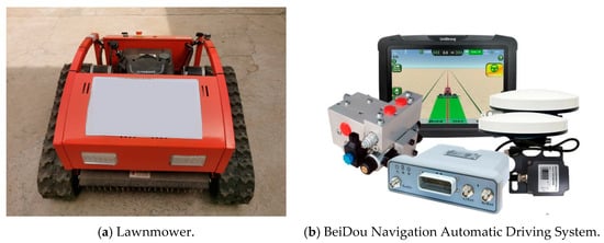
Figure 19.
Experimental equipment.
In the experiment, the measuring equipment included two 50 m-long tape measures, two 5 m-long steel tape measures, a timer for recording the working time of the lawnmower, three sets of pens and notebooks for recording experimental data, a fuel tank (10 L) filled with fuel, a mobile power supply, a DJI waypoint marker, and a 500 mL measuring cup, along with several meters of nylon line.
4.4.2. Experimental Plan
This experiment was designed with two groups to validate the accuracy of the optimal number of lawnmowers for covering orchards in both connected and non-connected orchards. The field test plan was as follows:
Step 1: Prepare the experimental equipment and select the experimental site.
Step 2: Collect experimental site data and set simulation parameters. Use a drone for aerial photography of the orchard terrain, obtaining information on the orchard and obstacle locations. Process the obtained data, including prescription maps, and create a simulated grid map. Test the fuel consumption of the lawnmowers in the orchard environment and their actual driving speeds. Set simulation experiment parameters based on this information.
Step 3: Conduct simulation experiments and obtain simulation data. Allocate the designated areas to lawnmowers based on the created simulated grid map. Use the improved A* algorithm to plan the lawnmowers’ optimal driving paths. Simultaneously, collect experimental data on the lawnmowers’ shortest working time, repetition rate, and omission rate during orchard traversal.
Step 4: Conduct on-site experiments and obtain actual experimental data. Input the paths planned during the simulation experiment into the control console, which sends signals to the lawnmowers to follow the planned paths. Record experimental data during the actual operation of the lawnmowers and any issues encountered.
Step 5: Analyze and compare the experimental results. Compare and analyze the repetition rate, omission rate, and shortest working time data of the lawnmowers between the simulation and the actual experiments to validate the feasibility of the plan.
4.4.3. Analysis of Simulation and Field Test Results
Three lawnmowers were used for field tests, and each lawnmower, when fully fueled, could work for approximately 1.5 h in the actual orchard environment, covering an area of around 0.6035 hectares. Through field testing, the average driving speed of the lawnmower in relatively flat orchard areas was determined to be v = 0.74 m/s. Since the slope of the orchard in the test area was mostly around 5 degrees, it had almost no impact on the lawnmower’s speed, so the slope of the orchard was not considered in this experiment regarding its effect on the lawnmower’s speed. However, in areas with dense weeds, the speed of the lawnmower would significantly decrease. After multiple measurements and averaging, the lawnmower’s speed in such areas was determined to be v = 0.48 m/s. The fuel consumption of the lawnmower in the working condition was:
Experiment 1.
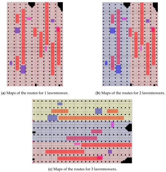
A connected region of the orchard was selected as the experimental area (as shown in Figure 20a). The total area of the experimental region was 1645.34 square meters, with obstacles primarily concentrated in the boundary areas of the orchard. Dense weed areas in this region were mostly located in the middle of the tree rows. A grid map was established based on the prescription map (Figure 20c). The size of grid map of experimental area 1 was set to 100 × 66.

Figure 20.
Route maps for the lawnmowers in Experiment 1. (White grids represent grids where the lawnmower can travel, gray grids indicate obstacle grids (i.e., impassable grids), pink grids represent uphill areas, blue grids denote down-hill areas, red grids represent overgrown grass areas, and yellow grids represent areas with sparse weeds. The lines in the picture show the routes of the robots).
Experiment 2.
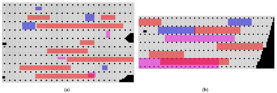
Two non-connected regions of the orchard were selected as experimental areas. The first experimental area was the same as that in Experiment 1. The second experimental area had an area of 1289.84 square units, with obstacles mainly concentrated in the boundary areas of the orchard. A grid map was established based on the prescription map (Figure 21b). The size of grid map of experimental area 2 was set to 120 × 45.

Figure 21.
Grid maps of experimental areas 1 and 2 for experiments 1 and 2. (a) Grid map of experimental area 1 (rotated counterclockwise by 90 degrees); (b) grid map of experimental area 2 (rotated clockwise by 90 degrees). (White grids represent grids where the lawnmower can travel, gray grids indicate obstacle grids (i.e., impassable grids), pink grids represent uphill areas, blue grids denote down-hill areas, red grids represent overgrown grass areas).
- (1)
- Simulation Experiment Results
Using the grid map created for the first experimental orchard environment as input, the improved A* path was planned through MATLAB simulation software, as shown in Figure 20.
The data on the omission rate, repetition rate, energy consumption, and minimum working time of one, two, and three lawnmowers during the traversal of the orchard obtained from the simulation software are presented in Table 13.

Table 13.
Simulation test data for Experiment 1.
The conclusion that can be drawn from Table 13 is that in this experimental area, when using a different number of lawnmowers to traverse and cover the orchard, using three lawnmowers compared to one lawnmower resulted in a decrease in the omission rate of 0.002%, a decrease in the repetition rate of 0.001%, and a reduction in the shortest working time of 2762.14 s. Compared to using two lawnmowers, the omission rate decreased by 0.001%, the repetition rate decreased by 0.017%, and the shortest working time decreased by 701.33 s. However, the overall fuel consumption was slightly higher than when using one or two lawnmowers, resulting in the highest total cost. Therefore, in this simulation experiment, using three lawnmowers corresponds to the shortest working time, the lowest omission rate, and the lowest repetition rate in the planned path, whereas one lawnmower corresponded to the path with the lowest cost.
For Experiment 2, based on the grid map created according to the non-connected orchard environment as input, as mentioned in Section 4.3, three lawnmowers were used as a cluster to cover the orchard, with the omission rate, repetition rate, lawnmower energy consumption, and shortest working time recorded for each lawnmower. The improved A* path of the lawnmower was planned using MATLAB simulation software, as shown in Figure 22.
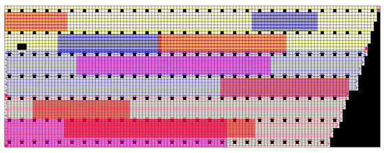
Figure 22.
Lawnmower trajectory map for the second experimental area 2 in Experiment 2. (White grids represent grids where the lawnmower can travel, gray grids indicate obstacle grids (i.e., impassable grids), pink grids represent uphill areas, blue grids denote down-hill areas, red grids represent overgrown grass areas, and yellow grids represent areas with sparse weeds. The lines in the picture show the routes of the robots).
The data for the lawnmower’s traversal in experimental area 2, including the omission rate, repetition rate, energy consumption for each lawnmower, and the minimum working time, are presented in Table 14.

Table 14.
Simulation experimental data for experimental area 2 in Experiment 2.
From Table 13 and Table 14, it can be observed that the lawnmower’s minimum working time for traversing experimental area 1 of the orchard was 1452.72 s, and for experimental area 2, it was 1221.53 s. After completing the traversal of experimental area 1, the lawnmower required energy replenishment, with a duration of 300 s. Therefore, the total minimum working time for the lawnmower in this non-connected orchard was 2974.25 s. Calculations based on Formulas (18) and (19) yielded a total repetition rate of 4.07% and a total omission rate of 0.24%.
- (2)
- Field Experiment
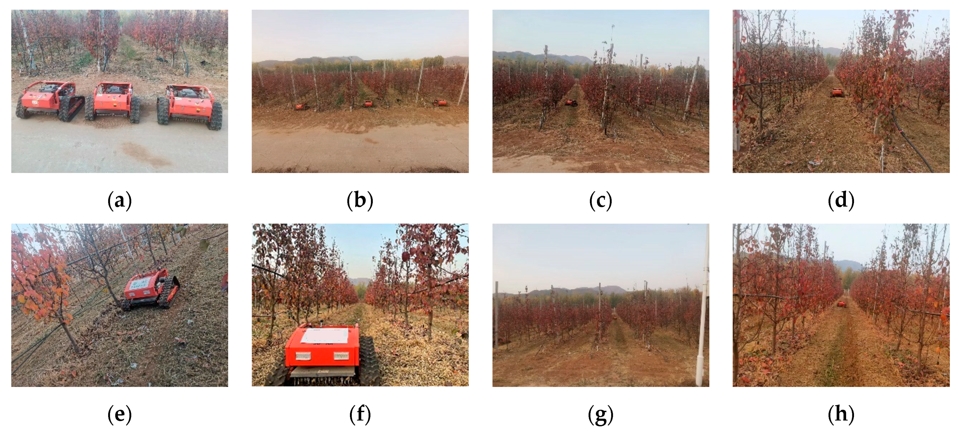
Experiment 1 was conducted in orchard test area 1. The process of Experiment 1 is illustrated in Figure 23.

Figure 23.
The field experiment for Experiment 1. (Figures (a–h) show part of the field test process in Experiment 1).
The resulting data of the coverage and traversal of experimental area 1 in the connected orchard by three lawnmowers are shown in Table 15.

Table 15.
Field experiment data for Experiment 1.
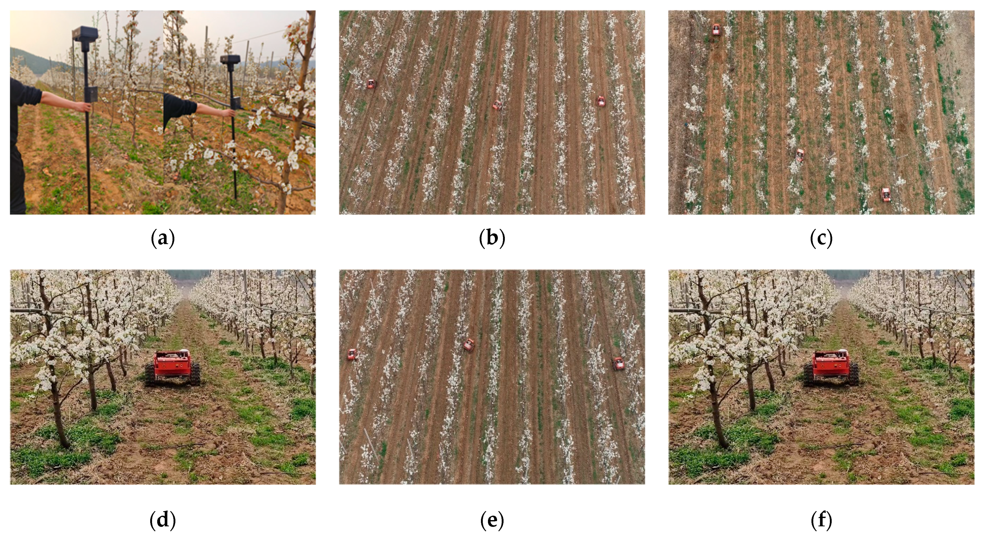
In experimental area 2 of the orchard, Experiment 2 was conducted, as illustrated in Figure 24. The energy replenishment time for the lawnmowers after completing the traversal of experimental area 1 was 258 s.
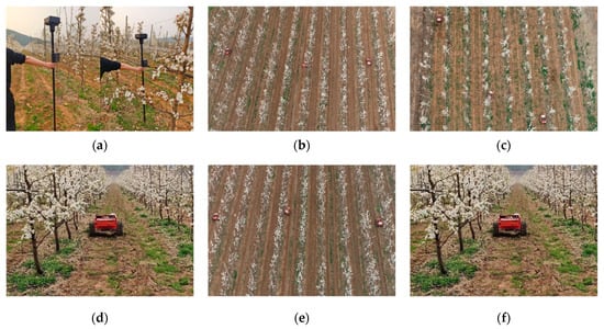
Figure 24.
Field test work of lawnmowers in area 2 in Experiment 2. (Figures (a–f) show part of the field test process in Experiment 2).
The resulting data of the coverage and traversal of experimental area 2 in the non-connected orchard by three lawnmowers in Experiment 2 are shown in Table 16.

Table 16.
Field test data for area 2 in Experiment 2.
The results from Table 15 and Table 16 show that the lawnmower’s shortest working time to traverse experimental area 1 in the orchard was 1721.43 s, and for experimental area 2, it was 1486.67 s. After traversing experimental area 1, the lawnmower required an energy replenishment time of 258 s. Therefore, the lawnmower’s total shortest working time for this non-connected orchard was 3466.1 s. Calculations using Formulas (18) and (19) yielded a total repetition rate of 5.71% and a total omission rate of 0.40%.
During the field test process, the following issues were recorded:
- (1)
- The unevenness of the orchard soil caused the lawnmower to experience fluctuations in its path during traversal.
- (2)
- The lawnmower’s traversal in the orchard compacted the weeds, leading to an increase in the lawnmower’s omission rate.
- (3)
- When turning, the lawnmower was affected by weeds, resulting in an increase in turning time.
- (4)
- Measurement errors: The inherent error in the positioning system caused the lawnmower to deviate from the planned path. There were also errors in measuring the lawnmower’s speed using a tape measure and a stopwatch.
Considering the actual conditions of the lawnmower’s traversal in the orchard, and taking into account that the area of the connected orchard experimental zone was 1645.34 square meters, a deviation of up to 5 min in the shortest working time was considered reasonable, an omission rate deviation of up to 1% was considered reasonable, and a repetition rate deviation of up to 2% was considered reasonable. For the non-connected orchard area with a total area of 2935.18 square meters, a deviation of up to 10 min in the shortest working time was considered reasonable, an omission rate deviation of up to 1% was considered reasonable, and a repetition rate deviation of up to 3% was considered reasonable.
- (3)
- Analysis of Experimental Results
A comparison between the actual data and simulation data for the lawnmower’s coverage path in the connected orchard experimental area is presented in Table 17 and was derived from Table 13 and Table 15. It constitutes a comparative analysis of the actual and simulated data from Experiment 1.

Table 17.
Comparative analysis of actual and simulated data from Experiment 1.
As can be seen in Table 17, the lawnmower’s actual data for traversing and covering the orchard show some discrepancies with the simulation data. There was a slight increase in the actual shortest working time compared to the simulated shortest working time of 412.71 s. The total energy consumption increased by 6333.6 kJ, the omission rate increased by 0.15%, and the repetition rate increased by 1.62%.
Table 14 and Table 16 provide the actual and simulated data for the lawnmower’s coverage path planning in the non-connected orchard experimental area, and a comparative analysis is presented in Table 18.

Table 18.
Comparative analysis of actual and simulated data for Experiment 2.
As can be seen in Table 18, the lawnmower’s actual data for traversing and covering the non-connected orchard exhibit some discrepancies with the simulation data. The actual shortest working time increased by 491.84 s. The total energy consumption increased by 9114 kJ, the omission rate increased by 0.15%, and the repetition rate increased by 1.62%.
Based on the above analysis, the main reasons for the discrepancies between the simulation data and actual experimental data are as follows:
- (1)
- The orchard’s uneven terrain caused fluctuations in the lawnmower’s path during traversal.
- (2)
- The lawnmower’s movement in the orchard compressed the weeds, leading to an increase in the omission rate.
- (3)
- While turning, the lawnmower was affected by weeds, resulting in increased turning time.
- (4)
- Measurement errors in the positioning system contributed to deviations from the planned path. Measurement of the lawnmower’s speed using a tape measure and stopwatch introduced errors.
In summary, the analysis indicates that the errors between the simulation and actual experimental data in both connected and non-connected orchards were relatively small, validating the rationality of orchard coverage path planning.
This section validates the practicality and reliability of orchard traversal path planning by conducting field experiments and comparing the data from field experiments with simulation test data. The section began by introducing the preparatory work for field experiments, describing the experimental site, equipment, methods, and objectives. Connected and non-connected areas within the orchard were selected to establish simulated grid maps. Subsequently, the selected orchard terrain underwent both simulation experiments and field experiments to collect data on the lawnmower’s omission rate, repetition rate, shortest working time, and energy consumption during orchard traversal. A comparative analysis was then conducted to identify the reasons for the discrepancies between the actual and simulated data. Through the comparative analysis of the simulation and actual experimental data, the errors in the lawnmower’s shortest working time, repetition rate, and omission rate during coverage in both connected and non-connected orchard areas were found to be within a reasonable range. Therefore, the path planning for this orchard was deemed rational.
5. Conclusions
This paper investigates the comprehensive coverage path planning method for tracked lawnmowers in orchards, exploring task allocation methods for lawnmower clusters. An improved A* algorithm is proposed, and the impact of lawnmower cluster quantity on path planning in different orchard scenarios is studied. Simulation verification of connected and non-connected areas, along with field experiments, demonstrates the practicality of the A* algorithm. However, future research requires further exploration and improvement. Firstly, extending path planning to three-dimensional space is necessary to consider the height of obstacles in the environment and the lawnmower’s height on path planning. Secondly, in complex agricultural systems, path planning algorithms need further refinement and optimization to fully leverage the potential of comprehensive coverage path planning technology in agriculture. Therefore, future research is expected to expand in these areas to achieve a more comprehensive application of path planning technology in agriculture.
Author Contributions
Conceptualization, M.Z. and S.W.; methodology, M.Z. and S.W.; software, M.Z. and S.W.; validation, M.Z. and S.W.; formal analysis, M.Z. and S.W.; investigation, M.Z.; resources, S.W.; data curation, S.W.; writing—original draft preparation, M.Z. and S.W.; writing—review and editing, X.L. and S.W.; visualization, X.L. and S.W.; supervision, L.W. and L.J.; project administration, L.W.; funding acquisition, S.W. All authors have read and agreed to the published version of the manuscript.
Funding
This work was funded by the National Natural Science Foundation of China under grant 32372592 and the CCF-Baidu Apollo Joint Development Project Fund.
Data Availability Statement
Data are contained within the article.
Conflicts of Interest
The authors declare no conflicts of interest.
References
- Li, Y.; Guo, Z.; Shuang, F.; Zhang, M.; Li, X. Key technologies of machine vision for weeding robots: A review and benchmark. Comput. Electron. Agric. 2022, 196, 106880. [Google Scholar] [CrossRef]
- McCool, C.; Beattie, J.; Firn, J.; Lehnert, C.; Kulk, J.; Bawden, O.; Perez, T. Efficacy of mechanical weeding tools: A study into alternative weed management strategies enabled by robotics. IEEE Robot. Autom. Lett. 2018, 3, 1184–1190. [Google Scholar] [CrossRef]
- Santos Valle, S.; Kienzle, J. Agriculture 4.0—Agricultural Robotics and Automated Equipment for Sustainable Crop Production; FAO: Rome, Italy, 2020. [Google Scholar]
- Saidani, M.; Pan, Z.; Kim, H.; Wattonville, J.; Greenlee, A.; Shannon, T.; Yannou, B.; Leroy, Y.; Cluzel, F. Comparative life cycle assessment and costing of an autonomous lawn mowing system with human-operated alternatives: Implication for sustainable design improvements. Int. J. Sustain. Eng. 2021, 14, 704–724. [Google Scholar] [CrossRef]
- Liao, W.; Zeng, F.; Chanieabate, M. Mechanization of small-scale agriculture in China: Lessons for enhancing smallholder access to agricultural machinery. Sustainability 2022, 14, 7964. [Google Scholar] [CrossRef]
- Wang, S.; Song, J.; Qi, P.; Yuan, C.; Wu, H.; Zhang, L.; Liu, W.; Liu, Y.; He, X. Design and Development of Orchard Autonomous Navigation Spray System. Front. Plant Sci. 2022, 13, 960686. [Google Scholar] [CrossRef] [PubMed]
- Patle, B.K.; Pandey, A.; Parhi, D.R.K.; Jagadeesh, A.J.D.T. A review: On path planning strategies for navigation of mobile robot. Def. Technol. 2019, 15, 582–606. [Google Scholar] [CrossRef]
- Orozco-Rosas, U.; Montiel, O.; Sepúlveda, R. Mobile robot path planning using membrane evolutionary artificial potential field. Appl. Soft Comput. 2019, 77, 236–251. [Google Scholar] [CrossRef]
- Lamini, C.; Benhlima, S.; Elbekri, A. Genetic algorithm based approach for autonomous mobile robot path planning. Procedia Comput. Sci. 2018, 127, 180–189. [Google Scholar] [CrossRef]
- Nazarahari, M.; Khanmirza, E.; Doostie, S. Multi-objective multi-robot path planning in continuous environment using an enhanced genetic algorithm. Expert Syst. Appl. 2019, 115, 106–120. [Google Scholar] [CrossRef]
- Wang, J.; Chi, W.; Li, C.; Wang, C.; Meng, M.Q.H. Neural RRT*: Learning-based optimal path planning. IEEE Trans. Autom. Sci. Eng. 2020, 17, 1748–1758. [Google Scholar] [CrossRef]
- Hart, P.E.; Nilsson, N.J.; Raphael, B. A formal basis for the heuristic determination of minimum cost paths. IEEE Trans. Syst. Sci. Cybern. 1968, 4, 100–107. [Google Scholar] [CrossRef]
- Tsuji, T.; Tanaka, Y.; Morasso, P.G.; Sanguineti, V.; Kaneko, M. Bio-mimetic trajectory generation of robots via artificial potential field with time base generator. IEEE Trans. Syst. Man Cybern. Part C 2002, 32, 426–439. [Google Scholar] [CrossRef]
- Janchiv, A.; Batsaikhan, D.; hwan Kim, G.; Lee, S.G. Complete coverage path planning for multi-robots based on. In Proceedings of the International Conference on Control, Automation and Systems, Gyeonggi, Republic of Korea, 26–29 October 2011; pp. 824–827. [Google Scholar]
- Hazon, N.; Kaminka, G.A. Redundancy, efficiency and robustness in multi-robot coverage. In Proceedings of the 2005 IEEE International Conference on Robotics and Automation, Barcelona, Spain, 18–22 April 2005; pp. 735–741. [Google Scholar]
- Hazon, N.; Kaminka, G.A. On redundancy, efficiency, and robustness in coverage for multiple robots. Robot. Auton. Syst. 2008, 56, 1102–1114. [Google Scholar] [CrossRef]
- Mathi, D.K.; Chinthamalla, R. A hybrid global maximum power point tracking method based on butterfly particle swarm optimization and perturb and observe algorithms for a photovoltaic system under partially shaded conditions. Int. Trans. Electr. Energy Syst. 2020, 30, e12543. [Google Scholar] [CrossRef]
- Mazdin, P.; Barciś, M.; Hellwagner, H.; Rinner, B. Distributed task assignment in multi-robot systems based on information utility. In Proceedings of the 2020 IEEE 16th International Conference on Automation Science and Engineering (CASE), Hong Kong, China, 20–21 August 2020; pp. 734–740. [Google Scholar]
- Bai, X.; Fielbaum, A.; Kronmüller, M.; Knoedler, L.; Alonso-Mora, J. Group-based distributed auction algorithms for multi-robot task assignment. IEEE Trans. Autom. Sci. Eng. 2022, 20, 1292–1303. [Google Scholar] [CrossRef]
- Zlot, R.; Stentz, A.; Dias, M.B.; Thayer, S. Multi-robot exploration controlled by a market economy. In Proceedings of the 2002 IEEE International Conference on Robotics and Automation (Cat. No. 02CH37292), Washington, DC, USA, 11–15 May 2002; Volume 3, pp. 3016–3023. [Google Scholar]
- Lin, B.; Zhao, Y.; Lin, R.; Liu, C. Integrating traffic routing optimization and train formation plan using simulated annealing algorithm. Appl. Math. Model. 2021, 93, 811–830. [Google Scholar] [CrossRef]
- Hustiu, I.; Kloetzer, M.; Mahulea, C. Distributed path planning of mobile robots with ltl specifications. In Proceedings of the 24th International Conference on System Theory, Control and Computing (ICSTCC), Sinaia, Romania, 8–10 October 2020; pp. 60–65. [Google Scholar]
- Atay, N.; Bayazit, B. Mixed-Integer Linear Programming Solution to Multi-Robot Task Allocation Problem; Washington University in St. Louis: St. Louis, MI, USA, 2006. [Google Scholar]
- Liu, J.; Yang, J.; Liu, H.; Tian, X.; Gao, M. An improved ant colony algorithm for robot path planning. Soft Comput. 2017, 21, 5829–5839. [Google Scholar] [CrossRef]
- Zhang, Y.; Pang, D. Research on path planning of mobile robot based on improved ant colony algorithm. In Proceedings of the 2022 IEEE 6th Information Technology and Mechatronics Engineering Conference (ITOEC), Chongqing, China, 4–6 March 2022; Volume 6, pp. 558–563. [Google Scholar]
- Wang, S.; Han, Y.; Chen, J.; He, X.; Zhang, Z.; Liu, X.; Zhang, K. Weed Density Extraction Based on Few-shot Learning through UAV Remote Sensing RGB and Multi-spectral Images in Ecological Irrigation Area. Front. Plant Sci. 2022, 12, 735230. [Google Scholar] [CrossRef] [PubMed]
- Medvedev, M.; Pshikhopov, V. Path planning of mobile robot group based on neural networks. In Proceedings of the Trends in Artificial Intelligence Theory and Applications. Artificial Intelligence Practices: 33rd International Conference on Industrial, Engineering and Other Applications of Applied Intelligent Systems, IEA/AIE 2020, Kitakyushu, Japan, 22–25 September 2020; Proceedings 33; Springer International Publishing: Berlin/Heidelberg, Germany, 2020; pp. 51–62. [Google Scholar]
- Wang, S.; Qi, P.; Zhang, W.; He, X. Development and Application of an Intelligent Plant Protection Monitoring System. Agronomy 2022, 12, 1046. [Google Scholar] [CrossRef]
Disclaimer/Publisher’s Note: The statements, opinions and data contained in all publications are solely those of the individual author(s) and contributor(s) and not of MDPI and/or the editor(s). MDPI and/or the editor(s) disclaim responsibility for any injury to people or property resulting from any ideas, methods, instructions or products referred to in the content. |
© 2024 by the authors. Licensee MDPI, Basel, Switzerland. This article is an open access article distributed under the terms and conditions of the Creative Commons Attribution (CC BY) license (https://creativecommons.org/licenses/by/4.0/).


