Prediction of Specific Fuel Consumption of a Tractor during the Tillage Process Using an Artificial Neural Network Method

Abstract

In mechanized agricultural activities, fuel is particularly important for tillage operations. In this study, the impact of seven distinct parameters on fuel usage per unit of draft power was examined. The parameters are tractor power, soil texture index, plowing speed, plowing depth, width of implement, and both initial soil moisture content and soil bulk density. This study investigated the construction of an artificial neural network (ANN) model for tractor-specific fuel consumption predictions for two tillage implements: chisel and moldboard plows. The ANN model was created based on the collection of related data from previous research studies, and the validation was performed using actual field experiments in clay soil using a chisel plow. The developed ANN model (9-22-1) was confirmed by graphical assessment; additionally, the root-mean-square error (RMSE) was computed. Based on the RMSE, the results demonstrated a good agreement for specific fuel consumption per draft power between the observed and predicted values, with corresponding RMSE values of 0.08 L/kWh and 0.075 L/kWh for the training and testing datasets, respectively. The novelty of the work presented in this paper is that, for the first time, a farm machinery manager can optimize tractor fuel consumption per draft power by carefully controlling certain parameters, such as initial soil moisture content, tractor power, plowing speed, implement width, and depth of plowing. The results show that the input parameters make a significant contribution to the output over the used data with different percentages. Accordingly, the contribution analysis showed that the implement width had a high impact on tractor-specific fuel consumption for both plows at 30.13%; additionally, the chisel and moldboard plows contributed 4.19% and 4.25% in predicting tractor fuel consumption per draft power. This study concluded that practical useful advice for agricultural production can be achieved through optimizing fuel consumption rate by selecting the proper levels of affecting parameters to reduce fuel costs. Moreover, an ANN model could be used to develop future tractor fuel-planning schemes for tillage operations.

1. Introduction

Tractors are among the most crucial pieces of equipment for carrying out the majority of agricultural tasks and activities [1,2]. Tractor use has led to a notable improvement in agricultural production [3]. In agricultural fields, the tractor serves as a power source for various farm implements [4]. For various reasons, a number of agricultural operations are necessary, including cultivating, spraying, seeding, and plowing. Specialist equipment is also required for various activities. Thus, a range of agricultural operations are reflected in the tractor-oriented test procedures that are commonly used to evaluate tractor energy inputs [2]. However, modern techniques to establish field experimental procedures with tractors and agricultural machinery and assess their performance and obtain results are now performed through computer simulations and mathematical models [2,5,6].

Tillage is the process of mechanically treating soil and creating an environment that is conducive to seed germination. Primary tillage is the initial mechanical disturbance of the soil following harvest, and this is usually carried out when the soil is sufficiently damp to permit plowing and robust enough to provide adequate and effective traction [7]. The terms for the tools involved in primary tillage operations are moldboards, disks, chisels, rotaries, and subsoiler plows [8]. As a result, an agricultural tractor equipped with such tools plays a vital role in agricultural production [7].

The quantity of fuel consumed by tractor engines throughout the tillage process depends on several factors. It is influenced by a number of factors, such as plow type, depth of plowing, and tractor forward speed [7,9]. The hourly fuel consumption raise in the course of tillage operation is caused by soil–implement–machine parameters such as draft, tillage speed, tillage depth, width of cut, soil bulk density, and soil moisture content [10]. Other parameters that have an effect on fuel consumption were shown by Kolator [2]. Furthermore, a tractor’s fuel consumption is affected by the local climate, tractor chassis, texture and structure of the soil, tractor size, and the combination of a tractor’s implements [11]. There are different results in research studies concerning the effects of specific parameters on fuel consumption due to the varying levels of such parameters [1,12]. Therefore, it is evident that the amount of fuel consumption fluctuates according to the levels of these parameters. In addition, fuel costs have a big impact on agricultural production’s input costs, particularly during primary tillage.

A key component of a tillage operation’s decision-making process when using optimization models is determining how to utilize fuel to maximize profit [11]. Farmers in developed countries have made significant use of models to budget tractor fuel consumption. Accurately measuring fuel consumption in the field is a very costly and challenging task. Although computer simulations are more effective, there remains a need for a universal technique to predict fuel consumption under various work conditions [13]. Since plowing is the initial tillage operation performed on the soil, the majority of investigations into modeling development for estimating tractor–implement combined fuel consumption focus on this particular process [14]. In the literature, numerous prediction models of tractor fuel consumption for tillage operations have been developed [11,14]. The relationship between the model response variable, such as fuel consumption, and other parameters found to be influencing tractor fuel consumption during the tillage process has been established using a variety of modeling techniques such as the multiple linear regression method, a category of regression analysis [14]. For example, Ekemube et al. [11] demonstrated that for the prediction of the quantity of fuel consumed during the harrowing process in a tilled area based on tillage speed and depth, the coefficient of determination (R²) was 100%, demonstrating that the predictable multiple linear regression (MLR) model formed for tractor fuel consumption per tilled area clarified 100% of the inconsistencies in the dataset. Therefore, an MLR algorithm was employed to develop a prediction model to estimate fuel consumption [14]. The study discovered that the predictive model developed for the harrowing process had an R²-value of 0.477, showing tractor power rating as the only operational factor contributing to the model they had established [14]. Almaliki et al. [15] applied MLR to predict the specific fuel consumption in units of kg/kWh, signifying the amount of fuel consumed during a specified time during a tillage process on the basis of the available drawbar power. The independent parameters were tillage depth, inflation pressure of a tractor tire, soil cone index, soil moisture content, engine speed, and tillage speed. The amount of fuel consumption could be estimated with an accuracy of about 95%. Previous authors have investigated alternative modeling techniques to test the capability of nonlinear mapping between multiple input and output parameters in order to achieve better results in comparison with MLR modeling techniques because the MLR models were unable to predict the fuel consumption needed for tillage implementation [16].

Various techniques have been employed by researchers to predict fuel consumption. All researchers’ attentions have been focused on artificial intelligence due to its development over the past ten years [17]. The artificial neural network (ANN) is a popular nonlinear model. The original design of the ANN was derived from the structure of the human biological neural system. Intelligent systems that can adapt and find nonlinear relationships between input and output datasets are known as ANN models. Future research can use a trained ANN based on accessible observation data in similar scenarios. Because of this exceptional quality, the ANN model has been used recently in a wide range of agricultural research domains. The literature contains extensive information on the ANN modeling technique’s development aspects [16,18,19,20]. An examination of some published papers revealed applications of the ANN in predicting fuel consumption requirements based on various field conditions. Shafaei et al. [16] used an ANN model to predict specific volumetric fuel consumption as a function of plowing depth and speed with a disk plow implement. The statistical descriptor parameters used to evaluate simulation environments revealed that the best ANN simulation environment could perfectly predict fuel consumption. They proposed that the devised ANN model could be used to develop future tractor fuel-planning schemes during tillage operations. Küçüksarıyıldız et al. [21] used an ANN model to calculate the precise fuel consumption at various axle loads, the inflation pressure of tractor tires, and the drawbar force for a 60 hp tractor. By experimenting with various transfer functions, the hidden-layer neuron count, and training algorithms, they discovered the most effective ANN model. Jalilnezhad et al. [17] used an ANN model for estimating the fuel consumption rate of a farm tractor. They calculated specific fuel consumption (L/kWh) by dividing temporal fuel consumption (L/h) by draft power. The inputs were soil texture components, soil moisture content, forward speed, working depth, number of passes of the tractor on the soil surface, tire inflation pressures, soil cone index, and dynamic load on the tractor’s rear tires. In spite of the intricacy of the variables and the lack of a clear correlation between the parameters, the developed ANN model has the potential to predict fuel consumption with a high degree of precision and minimal error.

The use of predictive models to estimate fuel consumption to budget the amount of tractor fuel required for a specific farm makes a significant contribution to farm machinery management and agricultural production. Soil tillage is the initial operation executed on the soil, and the common research papers on modeling development for tractor fuel consumption emphasize this process. Therefore, the current study was directed to assess the predictive ability of an ANN model for the direct prediction of tractor fuel consumption per draft power of a moldboard plow and a chisel plow under different working, tractor and implement, and soil conditions. The best model with the highest predictive ability offered in this study’s outcomes would be able to assist in agricultural machinery management to optimize fuel consumption rate by selecting the proper levels of affecting parameters.

2. Materials and Methods

2.1. The Information Needed to Model Tractor-Specific Fuel Consumption

For tillage experiments, the required data included initial soil moisture content, initial soil bulk density, soil contents of sand, silt, and clay, as well as tractor power, and implement width for the chisel and moldboard plows. All previous research studies have provided information on the amount of fuel used during the tillage process. Furthermore, the force needed for implements pulled in the tractor’s path of travel is known, as the draft or drawbar pull and these figures are provided and used in these studies.

The soil texture in this study is presented as the soil texture index as described in Dahham et al. [22], as follows:

$$\mathrm{STI}=\frac{\log \left({\mathrm{Ca}}^{\mathrm{Si}}+\mathrm{Sa}\right)}{100}$$

(1)

where STI represents the soil texture index (dimensionless); Sa displays the percentage of sand in the soil. The percentages of silt and clay in the soil are denoted by Si and Ca, respectively. The STI varies depending on the proportions of sand, silt, and clay in the soil and shows the effects of all three soil fractions.

The drawbar power is determined as follows:

$$\mathrm{DBP}=\frac{\mathrm{F}\times \mathrm{S}}{3.6}$$

(2)

where DBP is drawbar or draft power (kW); F is drawbar pull or draft force (kN); S is plowing speed (km/h); and 3.6 is the conversion unit.

2.2. The Validity of Fuel Consumption and Draft Measurements in the Collected Dataset

The tractor’s overall energy efficiency (OEE) is one of the primary factors influencing energy consumption [23]. Many researchers believe that higher OEE values are achieved when the tractor and tillage implements are used correctly [24]. Comparing the draft power and fuel consumption of a farm process is essential when evaluating the tractor–tillage–implement mechanization unit’s performance [25].

OEE incorporates load matching between a tractor and a plow, and it can be computed by dividing the draft power by the total energy present in the fuel volume used [26]. Fuel consumption measurements can be verified for validity using the OEE, which has a normal range of 10–20% [27]. An OEE of less than 10% for a tractor–plow combination indicates either poor load matching or low tractive efficiency. A value greater than 20% indicates either high tractive efficiency or a good match between loads. Equation (3) was used to calculate the overall fuel efficiency of a tillage system, and considers the tractive efficiency, engine/power train operating conditions, and load matching of the tractor and implement. This was executed by dividing the net energy used for the tillage operation in kilowatts by the energy formed by the net volume of fuel used in kW. A method that was similar to this suggestion appeared in Kazemi et al. [23] and Ranjbarian et al. [28]:

$$\mathrm{OEE}=\frac{\mathrm{DBP}\left(\mathrm{kW}\right)}{\mathrm{Pf}}\times 100$$

(3)

where Pf is the fuel corresponding power (kW) and can be calculated as follows:

$$\mathrm{Pf}\left(\mathrm{kW}\right)=\frac{\mathrm{FC}\left(\frac{\mathrm{L}}{\mathrm{h}}\right)\times \mathrm{HV}\left(\frac{\mathrm{kg}}{\mathrm{kJ}}\right)\times \mathrm{DD}\left(\frac{\mathrm{kg}}{\mathrm{L}}\right)}{3600}=10.21\times \mathrm{FC}\left(\frac{\mathrm{L}}{\mathrm{h}}\right)$$

(4)

where HV is the heating value of diesel fuel in the range of 42–46 MJ/kg. In this study, this value is assumed to be 44 MJ/kg for diesel fuel according to Uddin et al. [29]. FC is fuel consumption (L/h) and 3600 is the conversion unit. The density of diesel fuel is given by the symbol DD in Equation (4), which is affected by temperature [30], and in this study it assumed to be 0.835 kg/L [31].

Equation (5) was used to calculate the values of specific fuel consumption for different combinations (SFC, L/kWh). When an engine is running at maximum power, specific fuel consumption is the amount of fuel used per unit of time and power. It is primarily dependent on the kind and efficiency of the engine and is often represented in kg/(kW√h). The range for diesel engines is 0.21 to 0.26 kg/kWh, where older, less technologically advanced, and worn-out engines are represented by larger values, and new, low-aged engines by lower values [32]. Specific fuel consumption is the quantity of fuel used over a given period of time (FC, L/h), based on the drawbar power available at the drawbar.

$$\mathrm{SFC}=\frac{\mathrm{FC}}{\mathrm{DBP}}$$

(5)

The workflow for the research steps to attain values of specific fuel consumption from the literature data is shown in Figure 1. However,

Table 1. Statistical criteria of the collected dataset for chisel plow.

Parameters	Statistical Criteria
	Average	Maximum	Minimum	Standard Deviation	Coefficient of Variation (%)	Kurtosis	Skewness
OEE (%)	16.77	19.92	11.49	2.53	15.11	−1.12	−0.46
Plowing speed (km/h)	3.62	6.30	2.24	0.77	21.21	0.74	0.46
Draft force (kN)	11.09	19.52	6.88	3.00	27.05	0.15	0.85
Plowing depth (cm)	13.87	23.00	10.00	3.64	26.27	0.60	1.08
Fuel rate (L/h)	16.13	17.61	11.36	1.39	8.64	4.06	−1.92
Drawbar power (kW)	10.70	17.84	6.96	1.98	18.49	2.40	0.83
Specific fuel consumption (L/kWh)	1.57	2.42	0.64	0.35	22.22	0.55	0.03
Tractor power (kW)	79.50	86.79	56.00	6.87	8.64	4.06	−1.92
Initial soil moisture content (db, %)	16.47	20.50	6.80	3.83	23.26	−0.39	−0.98
Initial soil bulk density (g/cm3)	1.35	1.40	1.20	0.06	4.19	1.01	−1.39
Soil texture index (-)	0.30	0.66	0.10	0.16	53.29	0.80	0.87
Implement width (m)	2.09	3.85	1.75	0.72	34.39	2.25	2.00
No. of data points	89	89	89	89	89	89	89

and

Table 2. Statistical criteria of the collected dataset for moldboard plow.

Parameters	Statistical Criteria
	Average	Maximum	Minimum	Standard Deviation	Coefficient of Variation (%)	Kurtosis	Skewness
OEE (%)	18.76	20.00	14.43	1.10	5.88	−0.52	−0.82
Plowing speed (km/h)	4.05	5.25	2.57	0.59	14.68	0.52	0.17
Draft force (kN)	14.12	18.63	8.23	3.17	22.44	−0.15	−0.51
Plowing depth (cm)	16.93	21.00	7.30	2.61	15.40	2.81	−0.85
Fuel rate (L/h)	13.27	21.19	9.84	4.85	36.50	1.32	1.70
Drawbar power (kW)	16.06	21.73	7.89	4.66	28.99	−1.06	−0.51
Specific fuel consumption (L/kWh)	1.04	2.69	0.45	0.78	74.82	1.59	1.71
Tractor power (kW)	65.42	104.44	48.49	23.88	36.50	1.32	1.70
Initial soil moisture content (db, %)	14.56	19.80	8.26	2.98	20.44	−0.97	0.25
Initial soil bulk density (g/cm3)	1.27	1.52	1.08	0.10	8.25	−0.73	0.40
Soil texture index (-)	0.67	0.84	0.37	0.12	17.87	0.44	−1.28
Implement width (m)	1.04	1.35	0.80	0.16	15.04	5.24	−1.90
No. of data points	408	408	408	408	408	408	408

depict the statistical criteria of the collected dataset from previous research studies for chisel and moldboard plows, respectively.

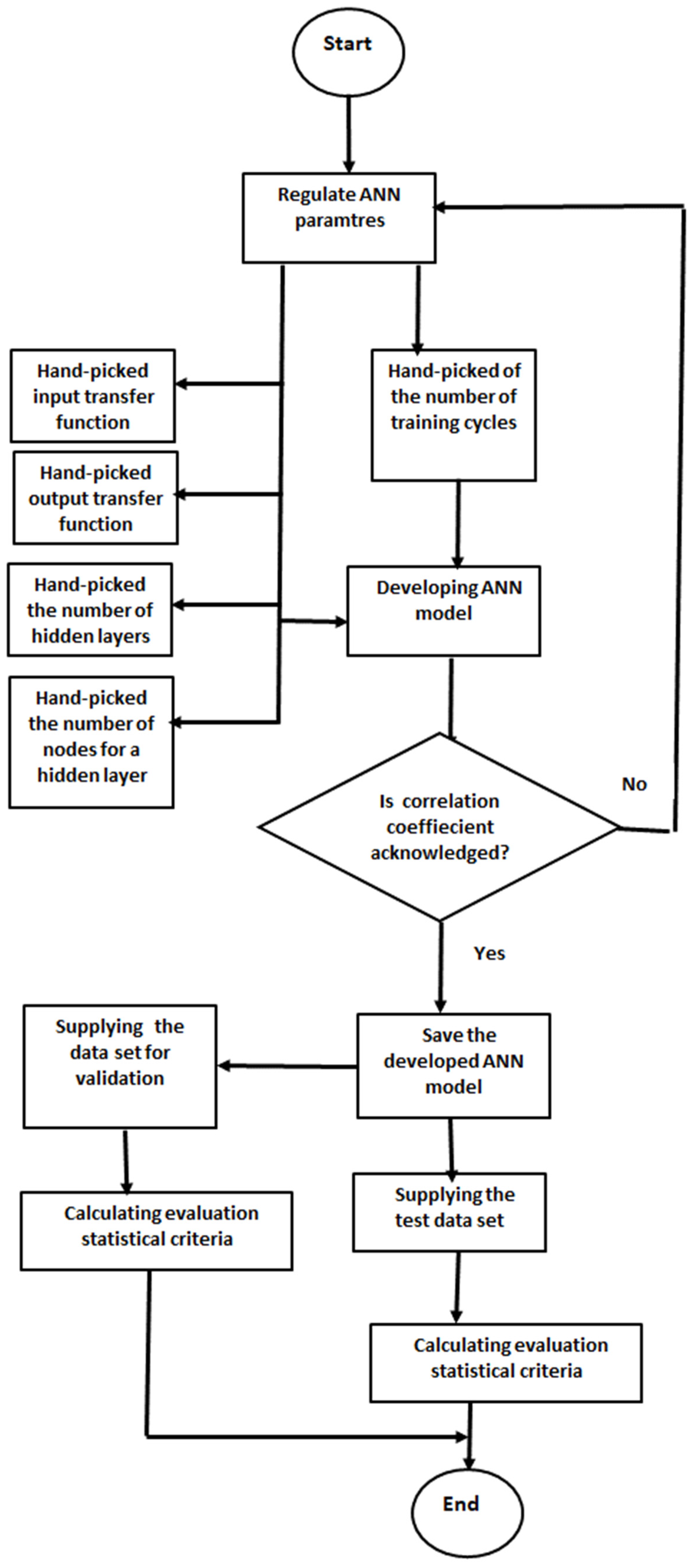
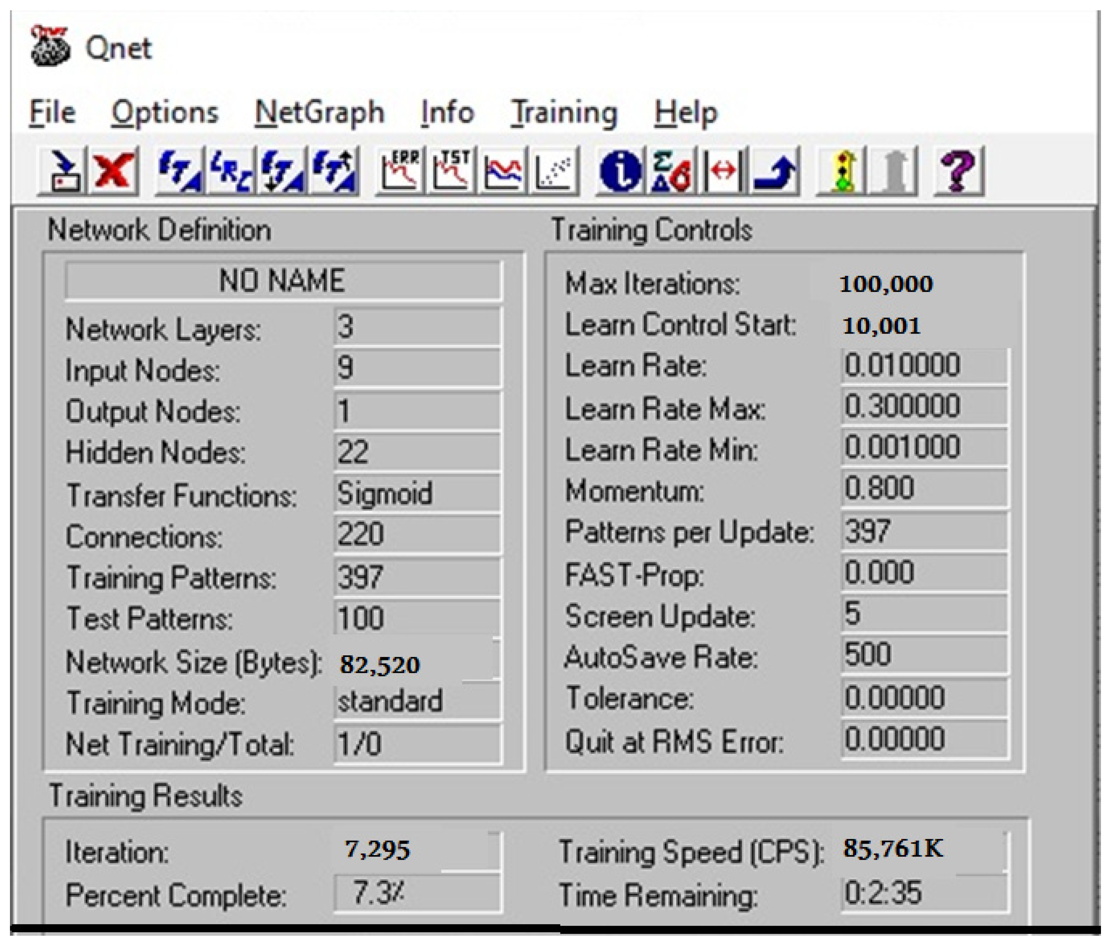
2.3. Structure of Tractor-Specific Fuel Consumption Prediction ANN Model

Monitoring farming operations is crucial for raising farm economic indicators and lowering pollution levels in the environment, particularly when it comes to the fuels used by machinery [33]. The modeling field of tractor fuel consumption has been led by ANNs, a well-liked machine learning technique, for the past few years [34]. ANNs are dependable, quick computing methods that produce precise predictions even with noisy, incomplete data, which are frequently seen in nonlinear problems [35,36]. Moreover, ANNs can be quickly developed using minimal quantities of experimental data and can approximate any complex nonlinear system [37]. However, a number of variables, such as the transfer function, the form of network architecture, and the learning algorithms employed, affect how well an ANN model performs. When compared to statistical models, ANNs trained with a backpropagation algorithm are said to have strong generalization capabilities [37].

The three main layers of a typical ANN model are the input layer, hidden layer, and output layer. Simple processing units, also referred to as neurons or nodes, are found at these levels. Weighted connections, which vary based on the needed ANN model designs, are used to connect the nodes to one another [38]. The particular challenges of this study are in determining how many hidden layers and how many nodes there are. According to a number of research studies [39,40], the most popular technique for determining the ideal number of hidden layers and their nodes is trial and error. Additional information about the ANN model and its uses can be found in Montesinos López et al. [38].

Given that ANN learning algorithms need numerical data, the one-hot encoding technique is used to convert categorical data (such as plow type, which in this study can be either a moldboard plow or a chisel plow) into integer data. Each input marker is represented by a binary vector (i.e., 0 or 1). According to Zheng and Casari [41], this method works well with categorical data when the categories are unrelated to one another. However, inputs containing numerical data are given to models exactly as they are. Given that choosing a network design and its parameters is typically performed empirically, using commercial software (Qnet v2000 for Windows), as described in Silva et al. [42], developed by Vesta Services makes it easy to find the optimal ANN model.

In this study, the network configurations, such as the multilayer perceptron (MLP) network model for modeling fuel consumption, were approached empirically, and the model that performed well with the training dataset was selected based on the coefficients of correlation and training error. The input layer of a typical MLP receives the signal from the inputs that need to be processed. Typically, the software in use employs the backpropagation learning algorithm to gradually construct an ANN model. To create an ANN model, several parameters are related. The regulated ANN model parameters are illustrated in Figure 2.

We obtained 497 data points for data collected from the literature for chisel and moldboard plows, which were randomly separated into training and testing datasets by our chosen software in a ratio of 80:20. In the study of Dahham et al. [22], the ANN model to predict the draft force of a disk plow was formed based on 375 samples reserved from field experiments. Using Equation (6), the data of input and output parameters were normalized into a range of 0.15 to 0.85:

$$\mathrm{NV}=\frac{\left(\mathrm{v}-{\mathrm{v}}_{\min }\right)}{\left({\mathrm{v}}_{\max }-{\mathrm{v}}_{\min }\right)}\times \left(0.85-0.15\right)+0.15$$

(6)

where NV is the input or output normalized vector (however, NVmax is 0.85 and NVmin is 0.15), and V, Vmax, and Vmin are the original data, the maximum value, and the minimum value of input or output data. The initial weights and biases of the neurons were chosen at random by the algorithm. There were 397 patterns in the training dataset, 100 data points in the testing dataset, and 3 data points in the validation dataset.

Using Qnet v2000, simulations were run. Differential attempts led to the selection of MLP with a single hidden layer as the ANN architecture. The input layer was composed of nine nodes (tractor power, initial soil bulk density, soil texture index, plowing depth, plowing speed, implement width, initial soil moisture content, chisel plow, and moldboard plow). During the ANN model development process, the number of neurons in the hidden layer was set to a range from one to thirty. The activation functions of neurons were sigmoid and hyperbolic tangent. Initial weights and biases of neurons were chosen randomly. The developed ANN model training speed was 85,761 K after being trained 100,000 times. During the ANN learning cycle, the network data were trained in order to ascertain the number of neurons and modify the weight coefficients in each neuron [43]. The final network included one hidden layer that included 22 neurons, 9 neurons for the input layer, and 1 neuron for the output layer, and the activation function was sigmoid. These values were achieved after multiple attempts to change the network topology and 7295 iterations.

In this study, the best ANN model structure was created by nine inputs in the input layer, one hidden layer with twenty-two nodes, and one input layer with one node (9-22-1). The training error was 0.020675, which was achieved after 7295 iterations, and the sigmoid transfer function with training mode standards is shown in Figure 3.

The matrices and vectors W1 and B1, and W2 and B2, respectively (Equation (7)), indicate the biases and weight coefficients associated with the ANN model’s hidden and output layers [43]. Matrix notation can be used to depict the ANN model. Equation (7) is used for computing the neural network’s output data [43]:

Y = f1(W2·f2(W1·X + B1) + B2)

(7)

where X is the input layer matrix; Y is the output value; and f1 and f2 are the transfer or activation functions in the hidden and output layers (in this study, it was sigmoid).

2.4. Calculating the Importance of Variable Contributions

ANNs are often seen as a “black box” when utilized for predictive modeling. Because there are many different types of ANN models, their structures are unpredictable and connection weights are randomly initialized which, among other factors, makes it challenging to choose the best one. However, researchers have recently offered a number of ways of ascertaining the contribution of each independent input variable in an ANN model. The present study employs the techniques that were introduced by the utilized software Qnet v2000 to calculate the importance of variable contributions.

2.5. Field Experiments for Verifying the Developed ANN Model

To create a validation dataset, field experiments were conducted using a locally made chisel plow at a research farm owned by the Rice Mechanization Center, Meet El Deeba, Kafer El Sheikh Governorate, Egypt (latitude: 31°06′59.3″ N; longitude: 30°51′17.6″ E). The chisel plow was 175 cm wide and weighed 460 kg (4.51 kN). It was divided into two rows of seven shanks. The soil texture was clay soil; therefore, a tractor power of 67 kW was used to pull the plow. The study assessed the draft force and fuel consumption rate at varying plowing speeds (three levels) and one plowing depth. However, the plowing speeds were achieved by shifting the tractor’s gears. The whole set of data, consisting of 3 points and gathered from the field experiment, is displayed in

Table 3. Range of inputs and outputs used as a validation dataset obtained from the field experimental site.

Parameters	Value 1	Value 2	Value 3
Sand content (%)	28.6	28.6	28.6
Silt content (%)	17.7	17.7	17.7
Clay content (%)	53.7	53.7	53.7
Soil texture index (-)	0.306	0.306	0.306
Tractor power (kW)	82	82	82
Plowing depth (cm)	16	16	16
Plowing speed (km/h)	3.7	4.7	6.9
Initial soil moisture content (%db)	19.8	19.8	19.8
Initial soil bulk density (g/cm3)	1.36	1.36	1.36
Implement width (m)	1.75	1.75	1.75
Draft force (kN)	18.76	19.67	21.68
Drawbar or draft power (kW)	19.28	25.68	41.55
Fuel consumption (L/h)	15.18	16.15	21.81
Specific fuel consumption per draft power (L/kWh)	0.787	0.629	0.525
Overall energy efficiency (%)	12.44	15.57	18.66

. Using a cylindrical core sampler, soil samples were taken at five different random places at each site from a 30 cm topsoil layer. The samples were then dried in an electric oven for 24 h at 105 °C to determine both the initial soil bulk density and soil moisture content.

Draft force data were obtained in certain places using a locally constructed hydraulic pull meter. Through the dynamometer, the front tractor guided the rear tractor equipped with the chisel plow at the appropriate depths and plowing rates. Throughout the plowing pass, the chisel plow was kept in the lift position to record the draft. To achieve the plowing depth, the tractor’s three-point linkage height lever was randomly positioned to obtain a plowing depth of 16 cm. A single pass of the chisel plow was achieved on the soil surface. Steel tape was used to check the depth of the plowing from the soil’s surface to the furrow’s bottom. For every plowing speed, ten measurements were taken.

A graded 500 cm³ glass cylinder was utilized to measure the tractor–chisel plow combination’s fuel usage. The diesel fuel cylinder was completely filled and set aside. The tractor’s fuel tank was filled with diesel fuel up to a specific level before each test run, or first speed. After that, the tillage equipment was used 50 m away. The fuel level in the fuel tank dropped by a particular amount as a result of the tractor engine’s fuel consumption during field operations. The fuel stored in the graded cylinder was used to fill the fuel tank to the prior level once more. The graded cylinder’s ultimate level was subtracted from its initial level to determine the fuel usage. In addition, the time required to complete the run was recorded. Equation (8) was utilized to compute the volumetric fuel consumption rate (FCv, cm³/s) [44]:

$$\mathrm{FCv}=\frac{\mathrm{V}}{\mathrm{T}}$$

(8)

where T is the time needed to move the tractor over 50 m (s) and V is the amount of fuel used in each test run (cm³).

2.6. Evaluation of the Developed ANN Model’s Performance

Several evaluation statistical criteria, including mean absolute error (MAE) and root-mean-square error (RMSE), were used to assess and compare the outcomes of the created ANN model in this work. Also, the coefficient of determination (R²) was determined. This gauges how accurately the model predicts the result. It expresses the percentage of the dependent variable’s variance that the model explains and also evaluates the goodness of fit [45]. The following are the formulae for these statistical criteria [45,46]:

$$\mathrm{MAE}=\frac{1}{\mathrm{N}}{{\displaystyle \sum }}_{\mathrm{i}=1}^{\mathrm{N}}\left|\left(\mathrm{Yi}-\hat{\mathrm{Y}}\right)\right|$$

(9)

$$\mathrm{RMSE}=\sqrt{\frac{1}{\mathrm{N}}{{\displaystyle \sum }}_{\mathrm{i}=1}^{\mathrm{N}}{\left(\mathrm{Yi}-\hat{\mathrm{Y}}\right)}^2}$$

(10)

where Yi refers to the observed value; Ŷ denotes to the predicted value; and N is the total number of data in testing and training datasets.

3. Results and Discussion

3.1. Statistical Data Analysis

The relationships among the investigated seven distinct parameters were analyzed for fuel usage per unit of draft power. The parameters were operation parameters (plowing speed and plowing depth), tractor and implement parameters (tractor power and implement width), and soil parameters (soil texture index, initial soil moisture content, and initial soil bulk density), as shown in Table 1 and Table 2. However, all investigated parameters have an impact on fuel usage, as reported in the literature. On the other hand, the average, maximum, minimum, standard deviation, coefficient of variation (%), kurtosis, and skewness for performance parameters are illustrated in Table 1 and Table 2 for the chisel and moldboard plows, respectively. Moreover, it is clear that the coefficient of variation was in the range of 4.19% to 34.39% for the chisel plow data and in the range of 8.25 to 36.50% for the moldboard plow data. However, the high variation in some data may be attributed to the data being collected from different sources.

The average values of OEE, draft, fuel consumption rate, and drawbar power for the plowing unit of a tractor and a chisel plow were 16.77%, 11.09 kN, 16.13 L/h, and 10.70 kW, respectively, as shown in Table 1, under different conditions of plowing speeds and depths, considering both initial soil moisture contents and soil bulk densities, and tractor powers. However, these values were 18.76%, 14.12 kN, 13.27 L/h, and 16.06 kW, respectively, as shown in Table 2, for the plowing unit of a tractor and a moldboard plow.

The range of OEE was assessed by other studies; however, when the tractor–implement combination’s OEE is less than 10%, it suggests either poor load matching or low tractive efficiency. When the number is greater than 20%, it suggests either strong load matching or high tractive efficiency [27]. In the study of López-Vázquez et al. [26], OEE for a disk plow/disk harrow/planter as a tillage system resulted in 18.23%; for a chisel plow/disk harrow/planter as a tillage system, it was 6.88%; and for no-tillage, it was 4.77%. Other research produced similar findings; for various tillage implements, the OEE ranged from 11% to 20.08% [28]. Kim et al. [47] assessed the range of draft force for a moldboard plow, finding that the overall mean draft force was 8.1 ± 1.4 kN (5.6–9.5 kN) in sandy loam soil, 10.1 ± 2.5 kN (6.4–13 kN) in loam soil, and 13.9 ± 2.5 kN (10.4–17.7 kN) in clay loam soil. Loam and clay loam soils displayed 1.24 and 1.71 times higher overall mean draft forces, respectively, than sandy loam.

According to Chenarbon [48], for moldboard plow, tillage fuel consumptions at 10, 20, and 30 cm depths were 12.29, 14.78, and 17.22 L/h, respectively; however, the soil texture was silty clay (45% clay, 25% sand, and 30% silt), and the soil moisture contents were 11.25, 12.86, and 13.68 db %. In general, as the tractor draft, plowing speed, plowing depth, soil moisture content, soil bulk density, and implement width increased, an increase in the value of tractor fuel efficiency also occurred [10].

In passive soil tillage, operations with primary tillage implements are dependent on the drawbar power of the amount of fuel consumption during the use of a specific implement. However, the fuel consumption for soil tillage is correlated with the intensity of soil tillage [49]. The range of draft power was evaluated by other researchers using different tillage implements; for example, Askari et al. [50] reported that a maximum drawbar power value of 9 kW was recorded with a subsoiler tine at a plowing speed of 3.5 km/h and a depth of 50 cm. However, a change in plowing speed and implement type affected the tractor drawbar power. The maximum drawbar power occurred in chisel plowing with a plowing speed of 4 km/h, the minimum occurred in disk plowing with a plowing velocity of 1.5 km/h, and the range was from 4 to 14 kW for chisel, disk, and moldboard plows in the plowing speed ranges of 1.5, 2.3, 3, and 4 km/h with 23 cm as the plowing depth [28].

Kurtosis and skewness were used to assess the outliers in the experimental data and determine the distribution’s most important points. Kurtosis describes the extent to which outliers are present in the data distribution, whereas skewness is the degree of asymmetry seen in a probability distribution that departs from the symmetrical normal distribution of data [51]. All of the datasets gathered for this study had flatter kurtosis and symmetrical skewness. However, the node-shoot dataset showed a high peak kurtosis and positively high skewness, indicating a higher likelihood of outlier values in this dataset than in others. The normal distribution, which is symmetrical and has zero skewness, is compared to the skewed distribution [52]. Negative skewness demonstrates that extra data are dispersed on the left side of the data mean, while positive skewness discloses that extra data are scattered on the right side of the mean. As shown in Table 1 and Table 2, the values of skewness reflect the mark of data asymmetry to be positive for the specific fuel consumptions for chisel and moldboard plows of 0.03 and 1.71, respectively; however, there was an impact of data skewness on prediction accuracy, as most machine learning techniques frequently accept that variables follow a normal distribution [52]. In this study, the kurtosis value was in the range of −0.39 to 4.06 for chisel plow parameters and in the range of −0.52 to 5.24 for moldboard plow parameters, as shown in Table 1 and Table 2, respectively.

3.2. Analysis of the Developed ANN Model Using Training and Testing Datasets

On a farm, the tractor and plow used for soil tillage are thought to be the main energy users and cost factors [53,54]. Thus, for power savings, the tillage unit (tractor and plow) must be used in proper combination [55]. As a result, users and manufacturers alike need to have access to information about the behavior and activity of plowing units [56,57]. However, gathering information from the variables influencing a plowing unit’s fieldwork via a field study is an arduous, expensive, and time-consuming task [58]. Therefore, to ascertain the impact of these variables—which include operation (plowing speed and depth), soil conditions, and the specifications of tillage tools and tractors—researchers, designers, and manufacturers can benefit from computer predictions and mathematical models [59]. Along with choosing the best plowing unit combination, it is important to assess the tillage tool and tractor’s performance to make the best use of the power units that are available in the field [15].

The results of the prediction performance of fuel consumption per draft power based on the testing dataset using the developed ANN model show that it provides high prediction accuracy compared to field measurements, as it gave the best performance with the coefficient of determination (R²) for all testing datasets of 0.983, as shown in Figure 4. Also, for the prediction of fuel consumption per draft power, R² was 0.947 and 0.986 for the chisel and moldboard plows, respectively, using testing datasets, as shown in Figure 5. Close scattering around the regression line emphasizes the satisfactory performance of the developed ANN model.

Table 4. Comparison between training and testing datasets for ANN model (9-22-1) performance.

Statistical Criteria	Training Dataset	Testing Dataset
RMSE (L/kWh)	0.080	0.075
MAE (L/kWh)	0.057	0.054
R2	0.985	0.983

illustrates the best results obtained from the ANN model for fuel consumption per draft power in this research with statistical criteria (RMSE, MAE, and R²). The results show that the ANN model had an acceptable performance for predicting fuel consumption per unit draft power under different field conditions. The results are consistent with the findings reported in Almaliki et al. [60] and Algezi and Almaliki [61]. The biases and weights of the developed ANN model for tractor-specific fuel consumption prediction (applying Equation (7)) are shown in

Table 5. The weights (W1) between inputs and the hidden layer of the established ANN model for tractor-specific fuel consumption prediction (applying Equation (7)).

Hidden-Layer Neurons	W1 = Weight between Inputs and Hidden Layer
	Chisel Plow	Moldboard Plow	Tractor Power	Soil Texture Index	Plowing Depth	Plowing Speed	Initial Soil Moisture Content	Initial Soil Bulk Density	Implement Width
	(-)	(-)	(kW)	(-)	(cm)	(km/h)	(db, %)	(g/cm3)	(m)
1	0.19035	0.19717	−0.066	−0.35153	−0.08198	−0.39646	−0.04227	−0.08694	−0.15066
2	−0.85962	0.72751	−0.40716	−0.03638	1.50896	1.0031	0.50304	0.16612	0.08197
3	0.00233	0.02025	−0.05847	0.26385	0.26267	0.38647	0.11467	0.18132	0.18917
4	0.38077	−0.21469	−0.26129	−0.502	−0.34415	−0.91834	−0.07168	−0.19367	−0.15324
5	−0.06246	−0.01446	−0.31216	0.57808	0.73648	1.168	−0.11966	−0.47513	0.96697
6	−0.19697	−0.07868	−0.16973	0.43001	0.58962	0.8332	−0.23802	−0.46489	0.83826
7	−0.33345	0.27957	−0.39279	0.4924	0.8537	0.33519	−0.05576	−0.15482	0.64401
8	−0.01909	−0.31904	−0.09156	−0.08692	−0.7128	−0.51896	0.17518	0.23999	−0.56896
9	−0.41839	−0.11352	−0.33347	0.34396	1.00388	0.98626	−0.14585	−0.10698	0.9686
10	−0.41947	−0.10327	−0.17008	0.08392	0.53608	0.55534	0.05861	−0.387	0.75625
11	0.43118	−0.29121	0.14553	−0.67883	−0.52845	−0.46833	−0.08864	0.31176	−0.42124
12	−0.22067	−0.0067	−0.45759	0.50522	1.02118	0.52727	0.25051	−0.47065	0.68776
13	0.13672	−0.09198	0.19434	−0.555	−1.1652	−0.8032	0.09824	0.46372	−0.5922
14	0.35919	−0.11701	0.00218	0.00115	−0.09005	−0.05033	−0.14423	0.04469	−0.07174
15	0.09815	0.08976	−0.33991	0.36695	0.12448	0.61201	0.1112	−0.45562	0.40137
16	−0.00078	−0.37508	−0.20905	0.01447	−0.51086	−0.67855	0.20613	−0.21273	−0.39427
17	0.03141	0.13665	−0.28487	−0.13061	0.28313	0.01639	−0.04468	0.1166	−0.2194
18	0.06939	0.24756	−0.50143	0.02617	0.16886	0.29653	0.12143	0.06383	0.12486
19	0.43712	−0.08713	−0.08521	−0.1167	−0.11657	−0.88368	−0.15611	−0.28614	−0.40588
20	−0.20107	−0.20741	−0.28109	0.14172	0.09101	−0.25293	0.21062	−0.08701	−0.23752
21	0.15758	−0.26284	−0.19279	−0.35602	−0.30383	−0.25393	0.01294	−0.22675	0.03401
22	−0.89838	0.0991	1.16689	1.44052	−0.29635	0.63546	−0.02438	−0.47725	−5.30476

and

Table 6. The hidden-layer biases (B1), weight between output and the hidden layer (W2), and output-layer biases (B2) of the established ANN model for tractor-specific fuel consumption prediction (applying Equation (7)).

Hidden-Layer Neurons	B1 = Hidden-Layer Biases	W2 = Weight between Output and Hidden Layer	B2 = Output-Layer Biases
1	0.16048	0.77215	0.85011
2	0.11971	−1.52163
3	−0.16271	−0.16302
4	0.29622	1.29996
5	−0.37419	−1.55898
6	−0.14713	−1.13387
7	−0.20668	−0.95499
8	0.21623	1.28453
9	−0.04239	−1.46011
10	0.08792	−0.8132
11	0.11282	1.46147
12	0.0023	−1.14313
13	0.0854	1.85898
14	0.3168	0.5853
15	−0.19352	−0.53014
16	0.14068	1.10854
17	−0.19475	0.31311
18	−0.19155	−0.09952
19	0.10089	1.20881
20	−0.16293	0.40959
21	−0.19571	0.64424
22	−0.72726	4.84614

. From the biases and weights, a mathematical model can be derived to predict tractor-specific fuel consumption (L/kWh) for chisel and moldboard plows.

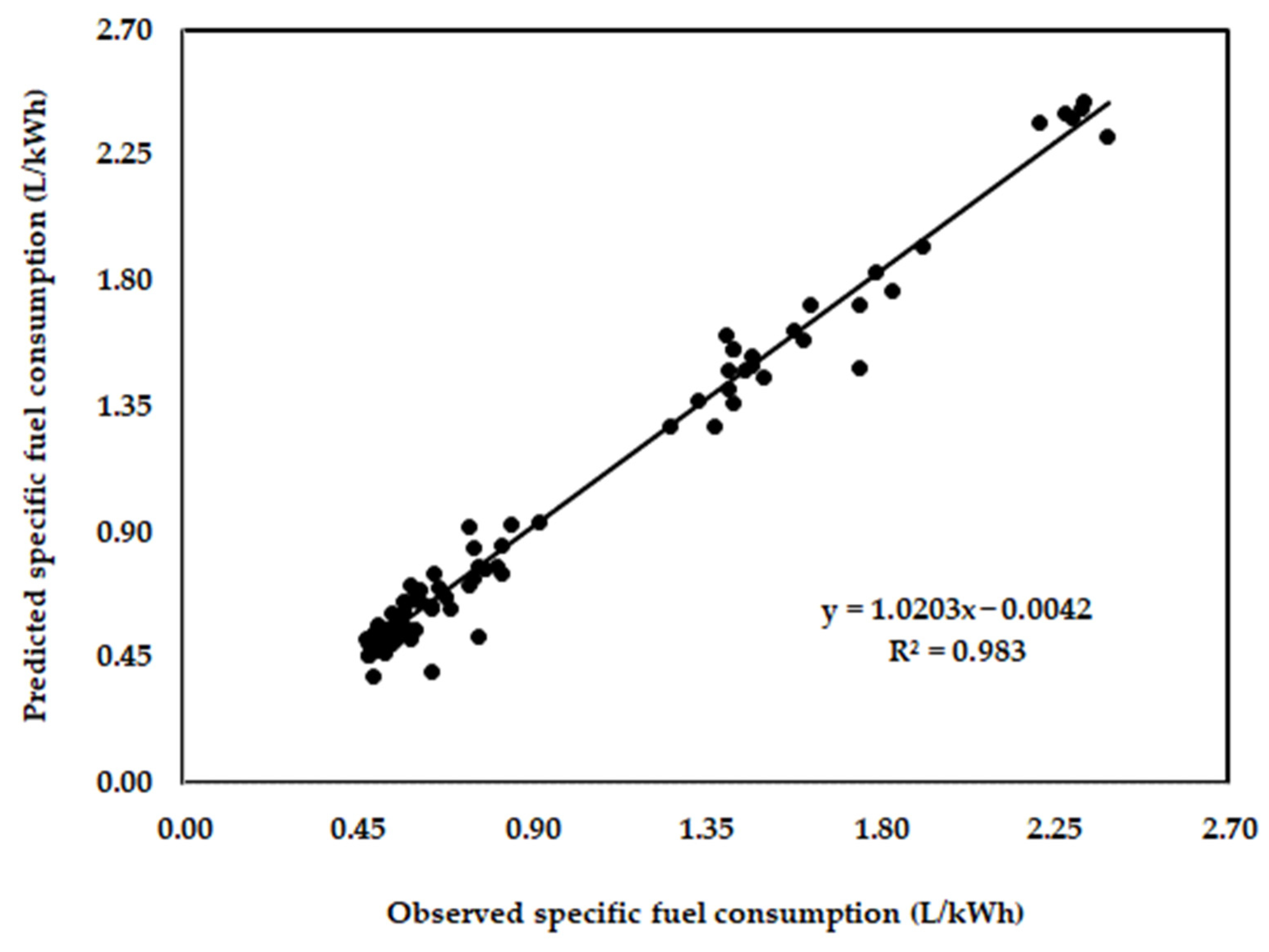
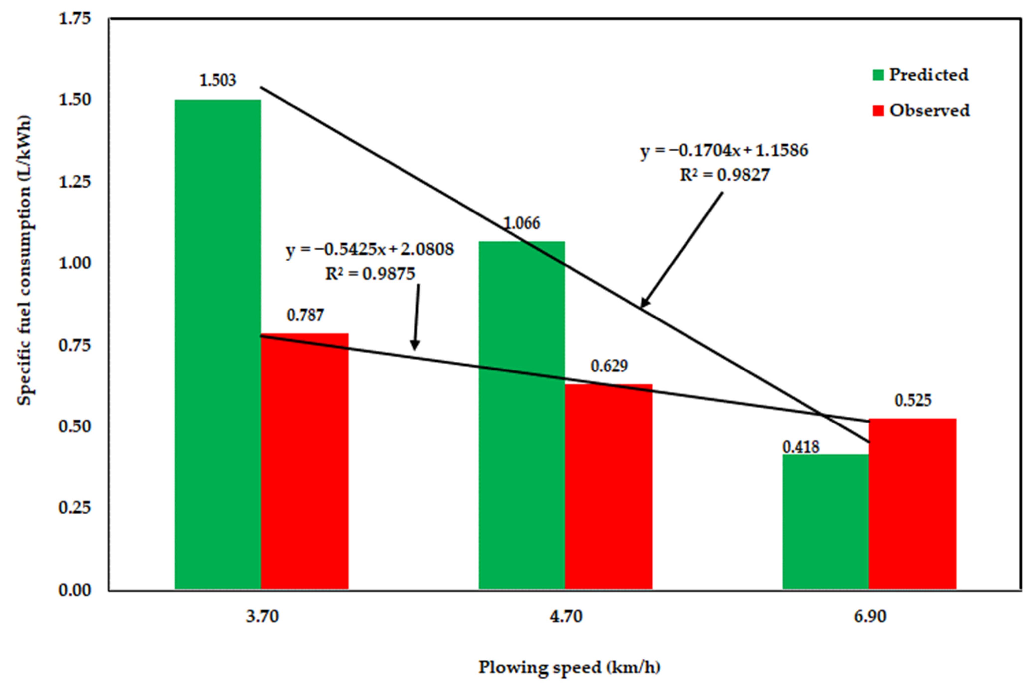
3.3. Analysis of the Developed ANN Model Using Validation Dataset

Volumetric measurements of fuel usage were taken for every field run. As demonstrated in Table 3, the results indicate that the chisel plow’s plowing speed increased from 3.7 km/h to 6.9 km/h by a percentage of 86.5%, as shown in Figure 6. Additionally, the fuel consumption (L/h) increased by 43.7%, the draft force (kN) by 15.6%, the drawbar power (kW) by 115.5%, and the OEE (%) by 50%. In contrast, the specific fuel consumption (L/kWh) decreased by 33.3%; however, consuming less fuel (L/kWh) is imperative and vital to decrease input costs for agricultural production processes (the data are shown in Table 3). On close examination of Figure 5, we discover the linear behavior of the specific fuel consumption with a determination coefficient higher than 0.95 for both datasets, observed and predicted using an ANN model after analyzing the impact of plowing speed on the specific fuel consumption (L/kWh) under investigation. In the study of Zimmermann et al. [62], they determined a second-order polynomial for specific fuel consumption per draft power through harrowing operations in the range of a forward speed of approximately 5.5 km/h to approximately 9.5 km/h, with a coefficient of determination greater than 99%. While the other examples in the study used less energy and did not differ among themselves, the slower speed required more energy for each produced potency. By using a chisel plow at 6.90 km/h, the lowest recorded specific fuel consumption (0.525 L/kWh) was achieved. The findings agree with the data obtained by Ranjbarian et al. [28]. The values observed and the predicted specific fuel consumption in this study compared to the range obtained by Klanfar et al. [32], who used a diesel fuel density of 0.850 kg/L (0.235–0.245 L/kWh) for given engine powers, perhaps due to the draft power being different to the implement-equivalent tractor power take-off. However, to assess the energy efficiency of tractors with various engine sizes and operating conditions, specific volumetric fuel consumption is utilized, as it is typically unaffected by engine size. The standard range of SVFC for diesel engines is 0.0476 to 0.1110 gal/hp-h [63]. In general, it is clear that the observed tractor-specific fuel consumption per draft power was a lower amount compared to the ANN prediction value with an average error of −0.349 L/kWh. However, this difference may be attributed to the values of draft power; thus, this demonstrates the ability of the created ANN model to predict tractor-specific fuel consumption per draft power. However, for professionals to evaluate the vehicle’s economy and to provide precise information regarding fuel utilization, an accurate fuel consumption model is essential [64].

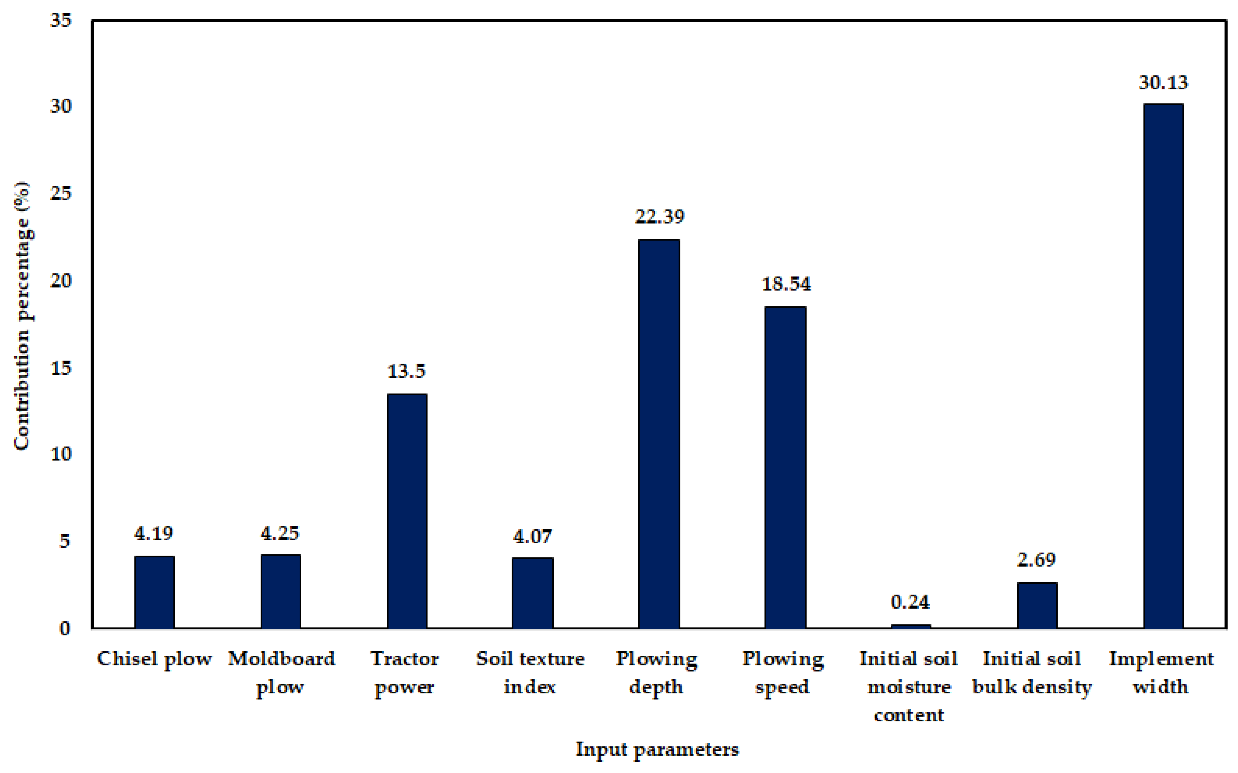
3.4. Contribution Analysis of the Affecting Parameters on Predicted Specific Fuel Consumption

The independent variable made different contributions to the tractor-specific fuel consumption prediction of tractor–chisel and –moldboard combinations using the ANN model of 9-22-1. As clearly shown in Figure 7, monitoring the implement width occupies the largest percentage of contribution (30.13%), showing the importance of using suitable implement width at selecting a plow for soil tillage. Additionally, the chisel and moldboard plows contributed 4.19% and 4.25% in predicting tractor fuel consumption per draft power (Figure 7). Moreover, plowing depth and speed were 22.39% and 18.54%, respectively (Figure 7). The two factors are important and have different effects on fuel consumption and draft force, as indicated in different research papers. Increasing the plowing speed from 0.51 to 1.45 m/s led to a decrease in fuel consumption per unit draft power of 135% [61]. This is due to the fact that an increase in plowing speed leads to an increase in traction requirements; thus, the amount of fuel consumed based on traction power decreases. The soil texture index contributed by 4.07% to specific fuel consumption predictions; however, Kim et al. [47] reported that draft forces were different and consequently so was fuel consumption.

4. Conclusions

Compared to other agricultural implements, primary tillage implements consume more energy, highlighting the need to optimize fuel consumption to reduce agricultural production costs. Tillage operations utilize a large amount of energy to create a suitable seed bed for planting crops. In order to maximize fuel consumption, it may be useful to predict tractor-specific consumption for a tractor–implement combination that is influenced by the tractor’s power, the soil’s texture, the depth and speed of the plowing process, both the initial soil moisture content and soil bulk density, and the implement width. The developed model of an artificial neural network with topology 9-22-1 and a backpropagation training technique was found to be suitable for predicting tractor-specific consumption (L/kWh) based on our findings. Furthermore, the training and testing datasets were used to assess the ANN prediction performance using RMSE and MAE, which were 0.080 L/kWh and 0.075 L/kWh for the training dataset and 0.057 L/kWh and 0.054 L/kWh for the testing dataset, respectively. According to the contribution analysis, the width of an implement has a significant impact on how much fuel moldboard and chisel plows use with tractors. The findings indicate that a farm machinery manager who effectively operates farming tillage equipment by selecting the appropriate range of parameters using this model would minimize fuel consumption and boost drawbar power. Furthermore, the developed ANN model showed promise in precisely predicting fuel usage per unit draft power for a plowing–tractor unit across a range of soil types. The developed ANN model had good potential to assist real-world decision making for agricultural machinery management and fuel use optimization.

References

1. Adewoyin, A.O.; Ajav, E. Fuel consumption of some tractor models for ploughing operations in the sandy-loam soil of Nigeria at various speeds and ploughing depths. Agric. Eng. Int. CIGR J. 2013, 15, 67–74. [Google Scholar]
2. Kolator, B.A. Modeling of tractor fuel consumption. Energies 2021, 14, 2300. [Google Scholar] [CrossRef]
3. Alhassan, E.A.; Asaleye, J.A.; Biniyat, J.K.; Alhassan, T.R.; Olaoy, J.O. Tractor acquisition and agricultural performance among Nigerian farmers: Evidence from co-integration modeling technique. Heliyon 2024, 10, e24485. [Google Scholar] [CrossRef]
4. Janulevičius, A.; Šarauskis, E.; Čiplienė, A.; Juostas, A. Estimation of farm tractor performance as a function of time efficiency during ploughing in fields of different sizes. Biosyst. Eng. 2019, 179, 80–93. [Google Scholar] [CrossRef]
5. Dahab, M.H.; Kheiry, A.N.O.; Talha, T.H.A. A computer model of fuel consumption estimation for different agricultural farm operations. Int. J. Environ. Agric. Res. 2016, 2, 77–85. [Google Scholar]
6. Kim, W.S.; Kim, Y.J.; Chung, S.O.; Lee, D.H.; Choi, C.H.; Yoon, Y.H. Development of simulation model for fuel efficiency of agricultural tractor. Korean J. Agric. Sci. 2016, 43, 116–126. [Google Scholar] [CrossRef]
7. Kareem, K.I.; Peets, S. Effect of ploughing depth, tractor forward speed, and plough types on the fuel consumption and tractor performance. Polytech. J. 2019, 9, 43–49. [Google Scholar] [CrossRef]
8. Moitzi, G.; Wagentristl, H.; Refenner, K.; Reinhardtian, H.; Piringer, G.; Boxberger, J.; Gronauer, A. Effects of working depth and wheel slip on fuel consumption of selected tillage implements. Agric. Eng. Int. CIGR J. 2014, 16, 184–190. [Google Scholar]
9. Tayel, M.Y.; Shaaban, S.M.; Mansour, H.A. Effect of plowing conditions on the tractor wheel slippage and fuel consumption in sandy soil. Int. J. ChemTech Res. CODEN 2015, 8, 151–159. [Google Scholar]
10. Ekemube, R.A.; Nkakini, S.O.; Igoni, A.H.; Akpa, J.G. Evaluation of tractor fuel efficiency parameters variability during ploughing operations. In Proceedings of the International Conference on New Views in Engineering and Technology (Icnet) Maiden Edition, Port Harcourt, Nigeria, 27 October 2021; pp. 111–122. [Google Scholar]
11. Ekemube, R.A.; Atta, A.T.; Ndirika, V.I.O. Optimization of fuel consumption for tractor-tilled land area during harrowing operation using full factorial experimental design. Covenant J. Eng. Technol. 2023, 7, 21–31. [Google Scholar]
12. Tihanov, G.; Ivanov, N. Fuel consumption of a machine-tractor unit in direct sowing of wheat. Agric. Sci. Technol. 2021, 13, 40–42. [Google Scholar] [CrossRef]
13. Lee, J.W.; Kim, J.S.; Kim, K.U. Computer simulations to maximise fuel efficiency and work performance of agricultural tractors in rotovating and ploughing operations. Biosyst. Eng. 2016, 142, 1–11. [Google Scholar] [CrossRef]
14. Oyelade, O.A.; Oni, K.C. Modelling of tractor fuel consumption for harrowing operation in a sandy loam soil. Arid. Zone J. Eng. Technol. Environ. 2018, 14, 8–19. [Google Scholar]
15. Almaliki, S.; Alimardani, R.; Omid, M. Fuel consumption models of MF285 tractor under various field conditions. Agric. Eng. Int. CIGR J. 2016, 18, 147–152. [Google Scholar]
16. Shafaei, S.M.; Loghavi, M.; Kamgar, S. A comparative study between mathematical models and the ANN data mining technique in draft force prediction of disk plow implement in clay loam soil. Agric. Eng. Int. CIGR J. 2018, 20, 71–79. [Google Scholar]
17. Jalilnezhad, H.; Abbaspour-Gilandeh, Y.; Rasooli-Sharabiani, V.; Mardani, A.; Hernández-Hernández, J.L.; Montero-Valverde, J.A.; Hernández-Hernández, M. Use of a convolutional neural network for predicting fuel consumption of an agricultural tractor. Resources 2023, 12, 46. [Google Scholar] [CrossRef]
18. Taghavifar, H.; Mardani, A.; Karim-Maslak, H.; Kalbkhan, H. Artificial neural network estimation of wheel rolling resistance in clay loam soil. Appl. Soft Comput. 2013, 13, 3544–3551. [Google Scholar] [CrossRef]
19. Taghavifar, H.; Mardani, A.; Hosseinloo, A.H. Appraisal of artificial neural network-genetic algorithm-based model for prediction of the power provided by the agricultural tractors. Energy 2015, 93, 1704–1717. [Google Scholar] [CrossRef]
20. Çarman, K.; Çitil, E.; Taner, A. Artificial neural network model for predicting specific draft force and fuel consumption requirement of a mouldboard plough. Selcuk. J. Agric. Food Sci. 2019, 33, 241–247. [Google Scholar] [CrossRef]
21. Küçüksarıyıldız, H.; Çarman, K.; Sabancı, K. Prediction of specific fuel consumption of 60 HP 2WD tractor using artificial neural networks. Int. J. Automot. Sci. Technol. 2021, 5, 436–444. [Google Scholar] [CrossRef]
22. Dahham, G.A.; Al-Irhayim, M.N.; Al-Mistawi, K.E.; Khessro, M.K. Performance evaluation of artificial neural network modelling to a ploughing unit in various soil conditions. Acta Technol. Agric. 2023, 26, 194–200. [Google Scholar] [CrossRef]
23. Kazemi, N.; Almassi, M.; Bahrami, H.; Shaykhdavoodi, M.; Mesgarbashi, M. Analysis of factors affecting the management of overall energy efficiency of tractor-implement by real-time performance monitoring. J. Agric. Mach. 2015, 4, 214–225. [Google Scholar]
24. Far, A.S.; Kazemi, N.; Rahnama, M.; Nejad, M.G. Simultaneous comparison of the effects of shaft load and shaft positions on tractor OEE in two soil conditions (cultivated and uncultivated). Int. J. Farming Allied Sci. 2015, 4, 215–221. [Google Scholar]
25. Pitla, S.K.; Luck, J.D.; Werner, J.; Lin, N.; Shearer, S.A. In-field fuel use and load states of agricultural field machinery. Comput. Electron. Agric. 2016, 121, 290–300. [Google Scholar] [CrossRef]
26. López-Vázquez, A.; Cadena-Zapata, M.; Campos-Magaña, S.; Zermeño-Gonzalez, A.; Mendez-Dorado, M. Comparison of energy used and effects on bulk density and yield by tillage systems in a semiarid condition of Mexico. Agronomy 2019, 9, 189. [Google Scholar] [CrossRef]
27. Askari, M.; Abbaspour-Gilandeh, Y.; Taghinezhad, E.; Hegazy, R.; Okasha, M. Prediction and optimizing the multiple responses of the overall energy efficiency (OEE) of a tractor-implement system using response surface methodology. J. Terramech. 2022, 103, 11–17. [Google Scholar] [CrossRef]
28. Ranjbarian, S.; Askari, M.; Jannatkhah, J. Performance of tractor and tillage implements in clay soil. J. Saudi Soc. Agric. Sci. 2017, 16, 154–162. [Google Scholar] [CrossRef]
29. Uddin, S.M.A.; Ahamed, J.U.; Alam, M.M.; Azad, A.K. Performance comparison of di diesel engine by using esterified mustard oil and pure musatrd oil blending with diesel. Mech. Eng. Res. J. 2013, 9, 104–109. [Google Scholar]
30. Schaschke, C.; Fletcher, I.; Glen, N. Density and viscosity measurement of diesel fuels at combined high pressure and elevated temperature. Processes 2013, 1, 30–48. [Google Scholar] [CrossRef]
31. Osman, S.; Stefaniu, A. Density, viscosity, and distillation temperatures of binary blends of diesel fuel mixed with oxygenated components at different temperatures. Sustainability 2023, 15, 15460. [Google Scholar] [CrossRef]
32. Klanfar, M.; Korman, T.; Kujundžić, T. Fuel consumption and engine load factors of equipment in quarrying of crushed stone. Teh. Vjesn. 2016, 23, 163–169. [Google Scholar] [CrossRef]
33. Damanauskas, V.; Janulevicius, A. Validation of criteria for predicting tractor fuel consumption and CO2 emissions when ploughing fields of different shapes and dimensions. AgriEngineering 2023, 5, 2408–2422. [Google Scholar] [CrossRef]
34. Niazian, M.; Niedbała, G. Machine learning for plant breeding and biotechnology. Agriculture 2020, 10, 436. [Google Scholar] [CrossRef]
35. Zhang, Q.; Deng, D.; Dai, W.; Li, J.; Jin, X. Optimization of culture conditions for differentiation of melon based on artificial neural network and genetic algorithm. Sci. Rep. 2020, 10, 3524. [Google Scholar] [CrossRef]
36. Sharma, P.; Said, Z.; Kumar, A.; Nižetić, S.; Pandey, A.; Hoang, A.T.; Huang, Z.; Afzal, A.; Li, C.; Le, A.T.; et al. Recent advances in machine learning research for nanofluid-based heat transfer in renewable energy system. Energy Fuels 2022, 36, 6626–6658. [Google Scholar] [CrossRef]
37. Gosukonda, R.; Mahapatra, A.K.; Ekefre, D.; Latimore, M., Jr. Prediction of thermal properties of sweet sorghum bagasse as a function of moisture content using artificial neural networks and regression models. Acta Technol. Agric. 2017, 2, 29–35. [Google Scholar] [CrossRef]
38. Montesinos López, O.A.; Montesinos López, A.; Crossa, J. Fundamentals of Artificial Neural Networks and Deep Learning. In Multivariate Statistical Machine Learning Methods for Genomic Prediction; Springer: Cham, Switzerland, 2022. [Google Scholar] [CrossRef]
39. Sheela, K.G.; Deepa, S.N. Review on methods to fix number of hidden neurons in neural networks. Math. Probl. Eng. 2013, 2013, 425740. [Google Scholar] [CrossRef]
40. Abdipour, M.; Younessi-Hmazekhanlu, M.; Ramazani, M.Y.H.; Omidi, A.H. Artificial neural networks and multiple linear regression as potential methods for modeling seed yield of safflower (Carthamus tinctorius L.). Ind. Crops Prod. 2019, 27, 185–194. [Google Scholar] [CrossRef]
41. Zheng, A.; Casari, A. Feature Engineering for Machine Learning: Principles and Techniques for Data Scientists; O’Reilly Media, Inc.: Sebastopol, CA, USA, 2018. [Google Scholar]
42. Silva, F.A.N.; Delgado, J.M.P.Q.; Cavalcanti, R.S.; Azevedo, A.C.; Guimarães, A.S.; Lima, A.G.B. Use of nondestructive testing of ultrasound and artificial neural networks to estimate compressive strength of concrete. Buildings 2021, 11, 44. [Google Scholar] [CrossRef]
43. Brandic, I.; Pezo, L.; Bilandžija, N.; Peter, A.; Šuri’c, J.; Vo´ca, N. Artificial neural network as a tool for estimation of the higher heating value of miscanthus based on ultimate analysis. Mathematics 2022, 10, 3732. [Google Scholar] [CrossRef]
44. Hensh, S.; Chattopadhyay, P.S.; Das, K. Drawbar performance of a power tiller on a sandy loam soil of the Nadia district of West Bengal. Res. Agric. Eng. 2022, 68, 41–46. [Google Scholar] [CrossRef]
45. Tsae, N.B.; Adachi, T.; Kawamura, Y. Application of artificial neural network for the prediction of copper ore grade. Minerals 2023, 13, 658. [Google Scholar] [CrossRef]
46. Sammen, S.S.; Kisi, O.; Ehteram, M.; El-Shafie, A.; Al-Ansari, N.; Ghorbani, M.A.; Bhat, S.A.; Ahmed, A.N.; Shahid, S. Rainfall modeling using two different neural networks improved by metaheuristic algorithms. Environ. Sci. Eur. 2023, 35, 112. [Google Scholar] [CrossRef]
47. Kim, Y.-S.; Lee, S.-D.; Baek, S.-M.; Baek, S.-Y.; Jeon, H.-H.; Lee, J.-H.; Kim, W.-S.; Shim, J.-Y.; Kim, Y.-J. Analysis of the Effect of Tillage Depth on the Working Performance of Tractor-Moldboard Plow System under Various Field Environments. Sensors 2022, 22, 2750. [Google Scholar] [CrossRef] [PubMed]
48. Chenarbon, H.A. Effect of moldboard plow share age and tillage depth on slippage and fuel consumption of Tractor (MF399) in Varamin region. Idesia 2022, 40, 113–122. [Google Scholar] [CrossRef]
49. Moitzi, G.; Haas, M.; Wagentristl, H.; Boxberger, J.; Gronauer, A. Energy consumption in cultivating and ploughing with traction improvement system and consideration of the rear furrow wheel-load in ploughing. Soil Tillage Res. 2013, 134, 56–60. [Google Scholar] [CrossRef]
50. Askari, M.; Abbaspour-Gilandeh, Y.; Taghinezhad, E.; El Shal, A.M.; Hegazy, R.; Okasha, M. Applying the response surface methodology (rsm) approach to predict the tractive performance of an agricultural tractor during semi-deep tillage. Agriculture 2021, 11, 1043. [Google Scholar] [CrossRef]
51. Said, Z.; Sharma, P.; Elavarasan, R.M.; Tiwari, A.K.; Rathod, M.K. Exploring the specific heat capacity of water-based hybrid nanofluids for solar energy applications: A comparative evaluation of modern ensemble machine learning techniques. J. Energy Storage 2022, 54, 105230. [Google Scholar] [CrossRef]
52. Chen, H.; Bu, Y.; Zong, K.; Huang, L.; Hao, W. The Effect of Data Skewness on the LSTM-Based Mooring Load Prediction Model. J. Mar. Sci. Eng. 2022, 10, 1931. [Google Scholar] [CrossRef]
53. Ahmadi, I. A draught force estimator for disc harrow using the laws of classical soil mechanics. Biosyst. Eng. 2018, 171, 52–62. [Google Scholar] [CrossRef]
54. Oduma, O.; Ehiomogue, P.; Okeke, C.G.; Orji, N.F.; Ugwu, E.C.; Umunna, M.F.; Nwosu-Obieogu, K. Modeling and optimization of energy requirements of disc plough operation on loamy-sand soil in South-East Nigeria using response surface methodology. Sci. Afr. 2022, 17, e01325. [Google Scholar] [CrossRef]
55. Gebre, T.; Abdi, Z.; Wako, A.; Yitbarek, T. Development of a mathematical model for determining the draft force of ard plow in silt clay soil. J. Terramech. 2023, 106, 13–19. [Google Scholar] [CrossRef]
56. Fawzi, H.; Mostafa, S.A.; Ahmed, D.; Alduais, N.; Mohammed, M.A.; Elhoseny, M. TOQO: A new tillage operations quality optimization model based on parallel and dynamic decision support system. J. Clean. Prod. 2021, 316, 128263. [Google Scholar] [CrossRef]
57. He, C.; Guo, Y.; Guo, X.; Sang, H. A mathematical model for predicting the draft force of shank-type tillage tine in a compacted sandy loam. Soil Tillage Res. 2023, 228, 105642. [Google Scholar] [CrossRef]
58. Badgujar, C.; Das, S.; Figueroa, D.M.; Flippo, D. Application of computational intelligence methods in agricultural soil-machine interaction: A review. Agriculture 2022, 13, 357. [Google Scholar] [CrossRef]
59. Cviklovič, V.; Srnánek, R.; Hrubý, D.; Harničárová, M. The control reversing algorithm for autonomous vehicles with PSD controlled trailers. Acta Technol. Agric. 2021, 24, 187–194. [Google Scholar] [CrossRef]
60. Almaliki, S.; Alimardani, R.; Omid, M. Artificial neural network-based modeling of tractor performance at different field conditions. Agric. Eng. Int. CIGR J. 2016, 18, 262–273. [Google Scholar]
61. Algezi, A.; Almaliki, S. Prediction of fuel consumption criteria of tractor using neural networks and mathematical models. Ann. For. Res. 2022, 65, 8902–8922. [Google Scholar]
62. Zimmermann, G.G.; Jasper, S.P.; Savi, D.; Francetto, T.R.; Cortez, J.W. Full-powershift energy behavior tractor in soil tillage operation. Eng. Agrícola 2023, 43, e20230054. [Google Scholar] [CrossRef]
63. Grisso, R. Predicting Tractor Diesel Fuel Consumption. Virginia Cooperative Extension; Publication 442-073; Virginia Tech: Blacksburg, VA, USA, 2020; 11p. [Google Scholar]
64. Nagar, H.; Rajendra Machavaram, A.; Soni, P.; Mahore, V.; Patidar, P. Cloud-driven serverless framework for generalised tractor fuel consumption prediction model using machine learning. Cogent Eng. 2024, 11, 2311810. [Google Scholar] [CrossRef]
Figure 1. The workflow for research steps to attain values of specific fuel consumption from the literature data.
Agronomy 14 00492 g001
Figure 2. Steps to build, test, and validate an ANN model.
Agronomy 14 00492 g002
Figure 3. Network definition and training control data as obtained using the employed software (Qnet v2000) for the developed ANN model to predict specific fuel consumption.
Agronomy 14 00492 g003
Figure 4. The relationship between observed and ANN predictions of fuel consumption per draft power for both chisel and moldboard plows (all testing datasets).
Agronomy 14 00492 g004
Figure 5. The relationship between observed and ANN predictions of fuel consumption per draft power for chisel and moldboard plows using testing datasets.
Agronomy 14 00492 g005
Figure 6. Regression of plowing speed in relation to tractor-specific fuel consumption per draft power (L/kWh) for chisel plow using observed and ANN-predicted values.
Agronomy 14 00492 g006
Figure 7. Independent variable importance for tractor-specific fuel consumption of a tractor–chisel or –moldboard combination using the ANN model of 9-22-1.
Agronomy 14 00492 g007