Cross-Regional Crop Classification Based on Sentinel-2

Abstract

Accurate crop classification is of vital importance for agricultural water management. Most researchers have achieved crop classification by model optimization in the same temporal and regional domain by adjusting the value of input features. This study aims to improve the accuracy of crop classification across temporal and spatial domains. Sentinel-2 satellite imagery is employed for crop classification training and prediction in selected farming areas of Heilongjiang Province by calculating vegetation indices and constructing sequential input feature datasets. The HUNTS filtering method was used to mitigate the influence of cloud cover, which increased the stability and completeness of the input feature data across different years. To address the issue of shifts in the input feature values during cross-scale classification, this study proposes the hypothesis testing distribution method (HTDM). This method balances the distribution of input feature values in the test set even without knowing the crop distribution, thereby enhancing the accuracy of the classification test set. The results indicate that the HTDM significantly improves prediction accuracy in cases of substantial image quality variance. In 2022, the recognition accuracy for crop types at all farms processed by the HTDM was above 87%, showcasing the strong robustness of the HTDM.

1. Introduction

Precise and rapid large-scale crop type recognition is an essential prerequisite for modern agricultural management and decision making, playing a key role in aspects such as regional planting structure statistical analysis and optimization [1,2], agricultural water resource allocation [3], farmland water and fertilizer management [4], and prevention and control of agricultural non-point-source pollution [5,6]. For instance, according to Xie et al. [7], spatial optimization of the planting structure at the national scale, based on crop type identification, could lead to an increase in farmers’ incomes by approximately 2.9% to 7.5% and a reduction in pesticide use by 4.3% to 10.8%. You et al. [8] indicated that large-scale crop classification aids in mapping crop distribution data. By further integrating water usage characteristics and fertilizer input of various crops [9], it is feasible to advance the acquisition of water consumption data from post-usage statistics to pre-usage assessment. This is vital for regional water resource allocation, water resource scheduling, as well as large-scale water and fertilizer management, and agricultural diffuse pollution assessment [10,11]. Additionally, large-scale precise and rapid crop type identification is closely related to agricultural finance [12] and agricultural insurance [13]. Crop classification at the field scale is a prerequisite for processing agricultural insurance claims. Ground surveying, the most classical method of obtaining crop type distribution, is not only resource-intensive but also suffers from temporal lags [14,15].

Due to the continuous temporal nature [16,17] and wide information coverage area of satellite remote-sensing images [18,19], in recent years, satellite remote-sensing technology has played a significant role in the identification of crop types over extensive areas [20], using extracted vegetation indices to train an improved CNN with single-date hyperspectral images, testing and validating the proposed method on two benchmark datasets. For the Indian Pines dataset, corn and soybeans achieved an average accuracy of 96.81% and 97.75%, respectively. For the Salinas dataset, fallow lands and lettuce achieved an average accuracy of 97.93% and 98.01%, respectively. Compared to hyperspectral remote sensing, multispectral remote-sensing technologies, due to their lower cost and wider availability of images, have seen broader application. Chakhar et al. [21] conducted data fusion of Landsat-8 and Sentinel-2 multispectral satellite images and explored the robustness and classification efficiency of diverse non-parametric classification algorithms for the fused datasets. Neetu and Ray [22] undertook efficient access to multispectral data on the Google Earth Engine (GEE) platform, filtering and preprocessing, where high-quality images based on the percentage of cloud cover were extracted, and explored the accuracy of different machine-learning classifiers in the task of crop classification.

In terms of implementation tools, many researchers have used machine-learning frameworks to achieve classification. There are two main research avenues here: one is to explore the adoption of new model frameworks and compare their classification accuracy with conventional machine-learning frameworks, and the other is to use different data sources, comparing various input dimensions, data fusion methods, and different resolution scales on crop classification imagery. Rohit Uttam Bhagwat designed an effective technique inspired by transfer learning (which utilizes a convolution neural network (CNN) as a feature extractor) and a popular gradient-boosting algorithm: XGBoost (as a classifier). And the results show this framework performed better than state-of-the-art methods, like random forest and Gaussian Naive Bayes. Stefanos Georganos compared XGBoost with benchmark classifiers such as random forest (RF) and support vector machines (SVMs) with very-high-resolution images. The results demonstrate that XGBoost parameterized with a Bayesian procedure and systematically outperformed RF and SVM, mainly in larger sample sizes.

However, when using multispectral satellite remote-sensing images for crop classification, cloud cover can cause information loss on the one hand [23], and on the other hand, localized cloud cover can significantly reduce the uniformity of image collection, dramatically increasing the heterogeneity of the samples, which can degrade classification accuracy [24,25]. Consequently, some researchers have turned to Synthetic Aperture Radar (SAR) imagery, which operates in longer wavelengths that can penetrate clouds [26,27]. Chakhar et al. [28] combined Sentinel-1 information (VV and VH backscatter and their ratio VH/VV) with NDVI calculated from Sentinel-2 satellite data to assess the classification accuracy of various classifiers using SAR data alone and in combination with optical data. Li et al. [29] used L-band SAR data for crop classification at an agricultural site in California’s San Joaquin Valley and achieved a peak classification accuracy of 90.5%. However, radar data use is often influenced by various factors such as the speckle noise effect in radar images [30], difficulties in interpreting the information [31], and numerical changes caused by terrain variations [32].

Furthermore, drone imagery has been utilized by scholars to mitigate the challenges posed by cloud interference. Despite the advantages of high resolution and temporal flexibility offered by Unmanned Aerial Vehicle (UAV) images as highlighted by Fan and Lu [18] and Kwak and Park [33], their coverage area remains relatively small compared to satellite remote-sensing images. This limitation, coupled with narrow coverage and variability in image quality due to multiple image dates, restricts their suitability for large-scale crop identification, as noted by Reedha et al. [34].

Additionally, existing research predominantly focuses on crop type identification within the same temporal and regional context, as evidenced by studies conducted by Bégué et al. [35], Li et al. [36], Yang et al. [19], and Zhong et al. [37]. However, there is a noticeable decrease in accuracy when extending remote-sensing crop classification to diverse regions, as observed by Ji et al. [38] and Wang et al. [39]. Sonobe et al. [40] employed TerraSAR-X data and machine-learning techniques to identify crops in Hokkaido, Japan, utilizing 2009 data for training and predicting classifications for 2012 images. Their results indicated an overall cross-classification accuracy of 89.1% for the same year, with a decrease to 78.0% accuracy for 2012. Similarly, Muhammad et al. [41] utilized data spanning from 2013 to 2019, with a subset of four years for training and one year for model evaluation, achieving accuracies ranging from 74.4% to 81.9%. These variations in accuracy can be attributed to differences in climate conditions and vegetation patterns across regions, leading to discrepancies in vegetation index values for the same crop type, as highlighted by Wang et al. [39].

Many of the abovementioned studies of crop classification focus on the same temporal and regional context and model optimization. When conducting cross-temporal and cross-spatial predictions, the accuracy of classification decreases to varying degrees. Researchers mostly optimized model structures to enhance proximity to precision. However, there exists an upper limit to accuracy when altering the model framework under the condition of equivalent image quality. Therefore, the primary objective of this study is to address the above issues from the perspective of data preprocessing. This approach aims to address the challenges related to data quality and completeness arising from cloud cover and temporal predictions based on single-image information. This paper employs filtered vegetation indices as inputs, with this processing step ensuring consideration of temporal information and ensuring the integrity and stability of data acquisition. After that, an iterative named the “hypothesis testing distribution method” is designed to address the issue of numerical offsets in cross-temporal and spatial prediction of imagery. This method achieves improved classification accuracy by adjusting corrections to input features through a gradient descent optimization logic with gradient descent.

2. Materials and Methods

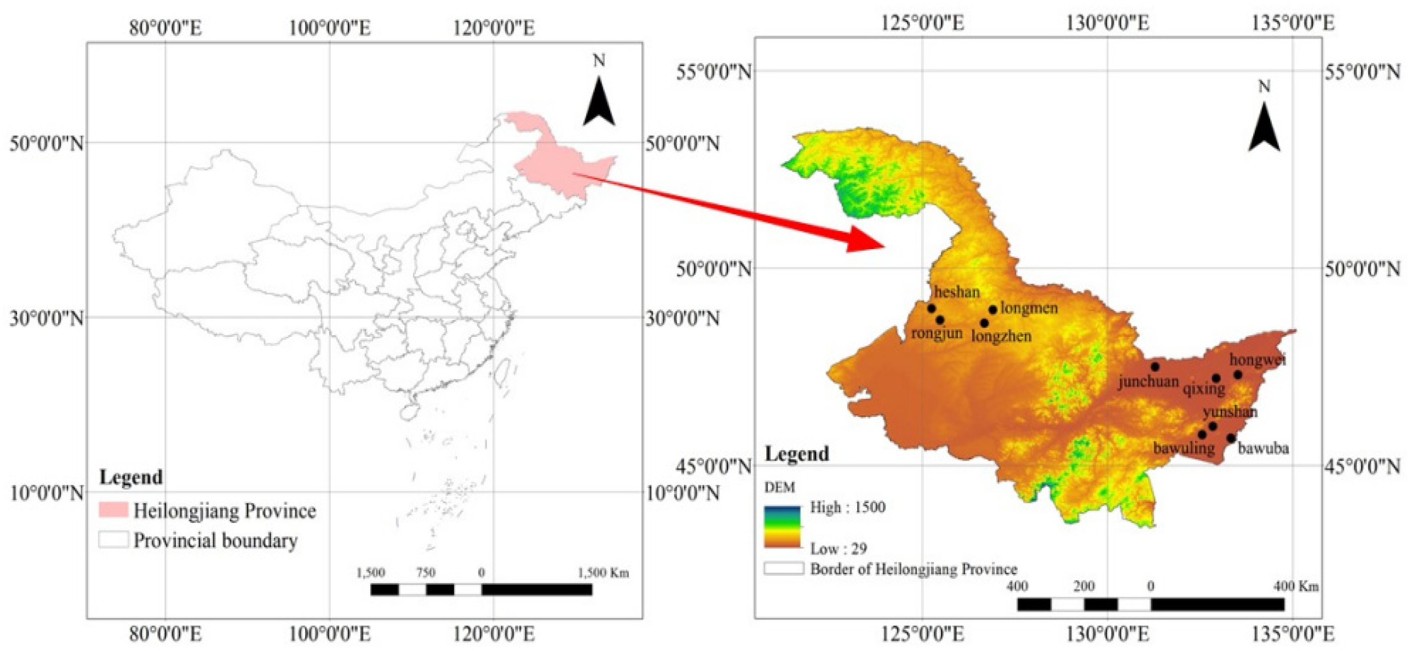
2.1. Study Area

The study area is located within Heilongjiang Province, which is the northernmost and highest-latitude province in China, characterized by a cold temperate and temperate continental monsoon climate. The annual average temperature is around 5 °C. Annual rainfall is approximately 550 mm. The average annual sunshine duration ranges from 2200 to 2500 h. Within the research area discussed in this paper, there are a total of ten farms (Figure 1), with a combined planting area of about 5,211,893 hectares. The main extensively planted crops are rice, corn, soybeans, and wheat. Based on vector files that include crop types, obtained through the analysis of planting policies and images of the same year, we can estimate the proportion of each crop in the random sampling points as representative of the distribution of farm crops (

Table 1. The proportion of planting area of various crops on each farm from 2019 to 2022.

Farm Name	Year	Proportion of Rice	Proportion of Maize	Proportion of Soybeans	Proportion of Wheat	AREA (m2)
Bawuling	2019	0.751	0.201	0.048	0	788,374,229.43
	2020	0.749	0.178	0.073	0	821,538,859.59
	2021	0.752	0.222	0.026	0	820,802,304.13
	2022	0.72	0.165	0.115	0	820,989,318.27
Bawuba	2019	0.936	0.025	0.039	0	801,388,296.55
	2020	0.939	0.015	0.046	0	801,942,534.54
	2021	0.927	0.031	0.041	0	801,667,709.59
	2022	0.895	0.027	0.078	0	806,883,923.12
Yunshan	2019	0.525	0.171	0.305	0	560,784,029.20
	2020	0.528	0.215	0.257	0	560,773,507.85
	2021	0.528	0.315	0.158	0	561,091,394.98
	2022	0.516	0.165	0.319	0	563,253,919.40
Junchuan	2019	0.827	0.158	0.016	0	842,704,046.51
	2020	0.827	0.129	0.044	0	842,557,865.42
	2021	0.829	0.159	0.012	0	842,484,184.65
	2022	0.822	0.093	0.085	0	845,874,235.93
Qixing	2019	0.858	0.055	0.088	0	1,489,302,362.59
	2020	0.847	0.062	0.092	0	1,494,554,545.85
	2021	0.825	0.081	0.094	0	1,493,962,739.02
	2022	0.832	0.076	0.092	0	1,494,063,878.37
Hongwei	2019	0.944	0.008	0.048	0	621,707,476.94
	2020	0.939	0.009	0.052	0	625,380,146.97
	2021	0.928	0.035	0.038	0	625,145,749.98
	2022	0.849	0.061	0.089	0	633,873,572.45
Longmen	2019	0	0.068	0.924	0.008	401,765,003.04
	2020	0	0.166	0.808	0.026	403,031,764.76
	2021	0	0.127	0.766	0.107	404,177,043.18
	2022	0	0.092	0.836	0.072	404,716,699.72
Longzhen	2019	0.018	0.362	0.619	0	684,490,977.34
	2020	0.021	0.303	0.676	0	680,682,141.26
	2021	0	0.2	0.729	0.071	680,930,624.84
	2022	0.017	0.321	0.661	0	681,397,904.22
Heshan	2019	0	0.374	0.626	0	1,071,868,559.92
	2020	0	0.377	0.622	0.001	1,067,989,960.08
	2021	0	0.379	0.621	0.001	1,067,959,640.31
	2022	0	0.318	0.681	0.001	1,064,687,937.30
Rongjun	2019	0.001	0.297	0.694	0.008	6,695,068,01.95
	2020	0.001	0.3	0.687	0.012	6,717,733,51.38
	2021	0	0.422	0.568	0.01	6,860,031,09.95
	2022	0.001	0.236	0.761	0.002	6,861,598,02.83

).

Table 1 reveals that Longmen Farm and Longzhen Farm primarily cultivate wheat, while the main crops of the other farms include rice, corn, and soybeans. Spatially, there is a significant difference in the crop distribution among the different farms, and even within the same farm, due to crop rotation and the conversion of paddy fields to dry land and other agricultural management practices, the spatial distribution of crops varies continuously between different years.

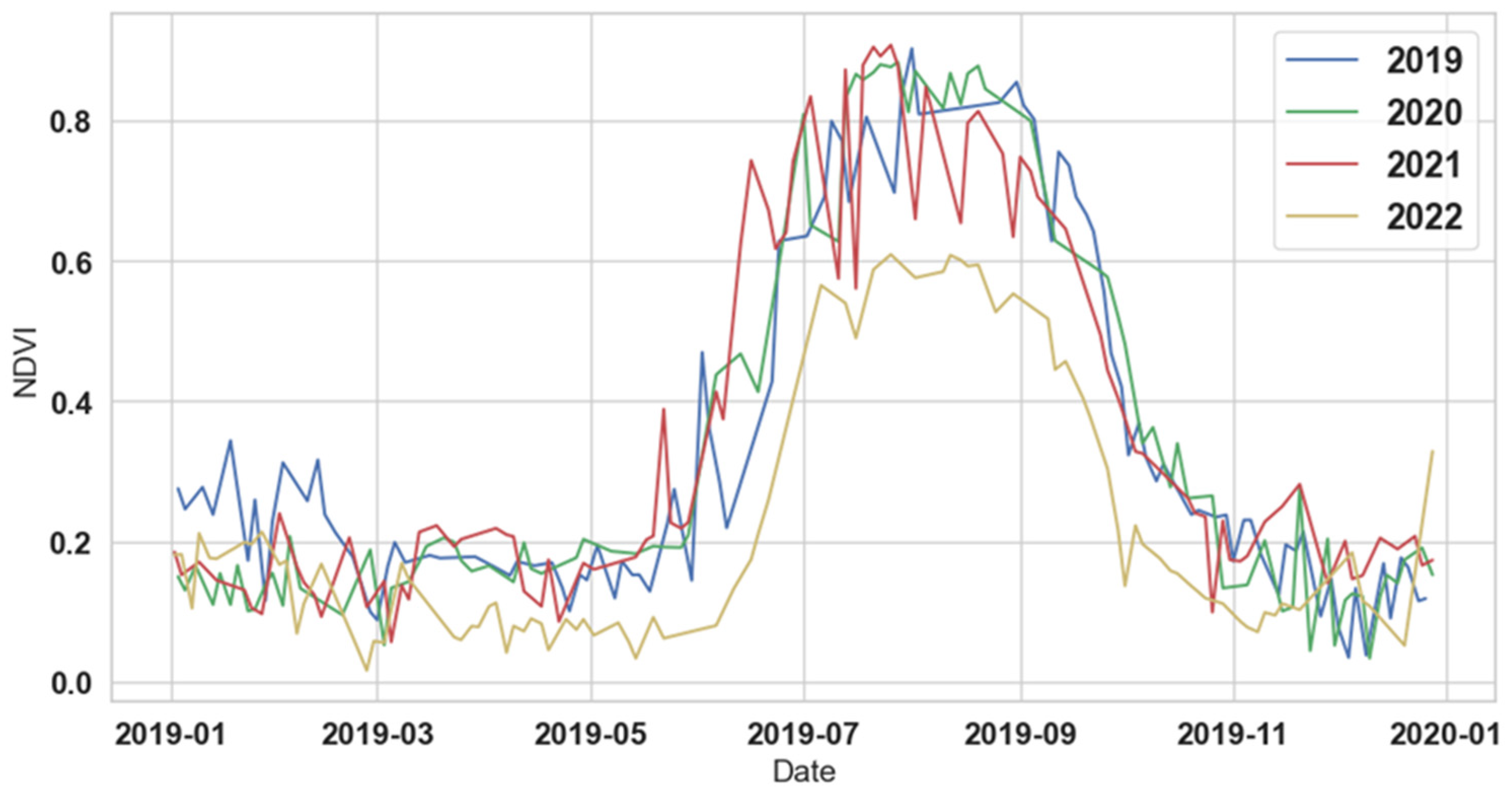
2.2. Image Sources and Input Feature

The remote-sensing image data utilized in this study are sourced from Sentinel-2 Level 2A images (L2A). L2A images are products that have undergone atmospheric correction based on the spatially corrected Level 1C images (L1C). The imagery encompasses a total of 13 bands, including three visible-light bands and one near-infrared band, each with a resolution of 10 m. Their respective central wavelengths are 496.6 nm (B2), 560 nm (B3), 664.5 nm (B4), and 835.1 nm (NIR). The bands with a resolution of 20 m include the red edge band (B5, B6, B7), narrow near-infrared (B8A), and short-wave infrared (B11, B12), with central wavelengths of 703.9 nm (B5), 740.2 nm (B6), 782.5 nm (B7), 864.8 nm (B8A), 1613.7 nm (B11), and 2202.4 nm (B12), respectively. Additionally, the coastal aerosol (B1) band with a resolution of 60 m and the water vapor band (B9) feature central wavelengths of 443.9 nm (B1) and 945 nm (B9), respectively. The Sentinel-2 mission operates with two polar-orbiting satellites in the same sun-synchronous orbit, which are phased at 180 degrees from each other. This configuration allows for a revisit period of three days in the region under study for this research.

Based on Sentinel-2 Level 2A remote-sensing imagery, this study selects six types of vegetation indices: LSWI, GLI, RNDVI, MSAVI, IRECI, and SAVI. The calculation formulas are given in Equations (1)–(6) [42,43,44,45]:

$$LSWI=\frac{NIR-SWIR}{NIR+SWIR}$$

(1)

$$GLI=\frac{2G-R-B}{2G+R+B}$$

(2)

$$MSAVI=2NIR+1+\frac{\sqrt{{(2NIR+1)}^2-8(NIR-R)}}{2}$$

(3)

$$IRECI=\frac{(EDGE3-R)EDGE2}{EDGE1}$$

(4)

$$SAVI=(1+L)\frac{NIR-R}{NIR+R+L}$$

(5)

$$RNDVI=\frac{EDGE1-R}{EDGE1+R}$$

(6)

where NIR is the near-infrared band, SWIR is the short-wave infrared band, G is the green band, R is the red band, B is the blue band, EDGE1 is the red edge 1 band, EDGE2 is the red edge 2 band, EDGE3 is the red edge 3 band, and L is an adjustment parameter used to modify the vegetation index to account for the influence of soil surface exposure, and it is commonly set to a value of 0.5.

Sentinel-2 imagery was acquired for the study area from 1 April to 1 September, and the various vegetation indices mentioned above were calculated. The indices were then organized chronologically, and the HUNTS temporal series smoothing algorithm was applied to eliminate numerical anomalies caused by disturbances such as cloud cover. After processing, the filtered results for the features on the 15th of each month from April to August were extracted, resulting in a total of 30 features. This process was conducted on the Google Earth Engine (GEE) platform, and the formula for the filtering curve is given in Equation (7) [46]:

$$HUNTS=a\sin (2\pi t)+b\cos (2\pi t)+2\pi tc$$

(7)

with HUNTS as the feature value after filtering at time t; t is the time, given in years, and a, b, and c are calibration parameters, which are independently determined for each pixel point.

3. Model Development and Evaluation

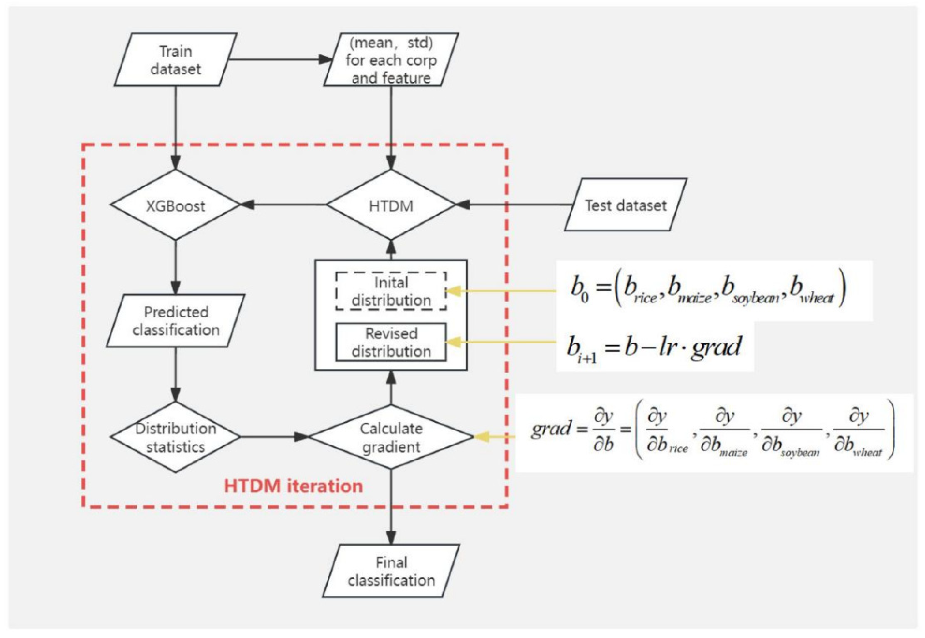
3.1. Hypothesis Testing Distribution Method

The crop classification algorithm used in this study was based on XGBoost. XGBoost is an optimized version of a Gradient Boosting Machine (GBM) model and likewise belongs to the category of ensemble machine-learning methods that aim to integrate multiple weak learners into an efficient model [47]. This algorithm iteratively constructs new base learners that are highly correlated with the negative gradient of the loss function, to maximally boost model performance. In XGBoost, the application of the squared loss function not only penalizes large deviations in the target output but also overlooks small residuals, thus making the calculation of pseudo-residuals and the optimal solution direction more efficient in each iteration. By the ingenious use of the squared loss function, XGBoost pays more attention to the accurate handling of errors during training, thereby enhancing the robustness and generalization ability of the model [47,48]. In this study, the experimental hardware platform consisted of an AMD Ryzen 5 3600 6-Core Processor CPU running in the Windows 10 operating system, along with an NVIDIA GeForce RTX 2060 GPU and 32 GB of RAM. The code was written using XGBoost 1.7.6 machine learning and developed using Python 3.9.12.

However, statistical analysis revealed that there is a bias in the values of vegetation indices for the same crop across different years (Figure 2). This bias originates from interannual differences in crop growth, atmospheric conditions, and satellite sensors. When the bias is significant, using raw vegetation index statistics without any processing can, to varying degrees, decrease the accuracy of crop classification.

Therefore, the current study proposes the use of the Index Normalization Method (INM) to eliminate the influence of interannual biases in vegetation indices. This method assumes that the distribution of the same type of crop is consistent (reflected in grid data by the proportion of pixels representing each crop type being constant). By using the training set to adjust the values within the prediction set, the calculation is given in Equation (8):

$$NewPixel=\frac{pixe{l}_{pred}-mea{n}_{pred}}{st{d}_{pred}}st{d}_{train}+mea{n}_{train}$$

(8)

where NewPixel is the corrected feature value, pixel_pred is the feature value of the original prediction dataset, mean_pred is the average value of the feature value in the prediction dataset, std_pred is the standard deviation of the specified feature in the prediction dataset, mean_train is the average value of the feature value in the training dataset, and std_train is the standard deviation of the specified feature in the training dataset.

Considering scenarios such as the transformation of paddy fields to dry fields, dry fields to paddy fields, and crop rotation, the crop distribution in the same farm can vary across different years in practice. To address this, our study proposes the HTDM, which extends the applicability of the Index Normalization Method, previously limited to identical distributions, to situations where crop distributions differ.

This method assumes that the crop distribution of the prediction set is the same as the initial distribution. Subsequently, it generates a new dataset based on the training set where the crop distribution equals the initial distribution and calculates the variance and standard deviation for each feature of this dataset. The calculation approach utilizes statistical principles and ensures computational speed by carrying out numerical calculations throughout the entire process. The calculation formula is given in Equations (9) and (10):

$$mean={\displaystyle \sum _{crop}^{rice,maize,soybean,wheat}mea{n}_{crop}{p}_{crop}}$$

(9)

$$std=\sqrt{{\displaystyle \sum _{crop}^{rice,maize,soybean,wheat}\frac{st{d}_{crop}^2(n·p_{crop}-1)+{(mea{n}_{crop}-mea{n}_{train})}^2·(n·p_{crop)}}{n-3}}}$$

(10)

where std_crop is the standard deviation of the specified feature for the crop within the training set, n is the number of data points in the training set, p_crop is the proportion of data for the crop in the training set, and mean_crop is the average value of the crop feature in the training set.

The variances and standard deviations calculated were applied to correct the validation set data using the Index Normalization Method (INM). The feature values were then fed into the trained model to output the classification results. The distribution of crop classification results was tallied and compared with the initially set distribution. We postulate that when the initially set distribution was similar to the predicted distribution generated based on the initial distribution, the initial distribution was considered as the actual crop distribution of the prediction set. To evaluate the quality of the model’s predictions during the hypothesis testing process, this study designed a loss function for hypothesis testing, which is expressed in Equation (11):

$$loss=\sqrt{{\displaystyle \sum _{crop}^{rice,maize,soybean,wheat}{w}_{crop}{(p_{pred,crop}-p_{crop})}^2}}$$

(11)

where loss is the loss value, w_crop is the weight of the crop, which is a hyper-parameter, p_pred,crop is the proportion of crop prediction results, and p_crop is the assumed proportion for the crop.

3.2. Gradient Descent

During the iterative process of determining crop distribution, we have chosen the gradient descent method as the means to refine the distribution. Gradient descent is an iterative optimization algorithm based on the gradient of the objective function, used to solve minimization or maximization problems. It is commonly applied in parameter optimization within machine learning, function minimization, and various other optimization issues. In solving the optimization problem of finding the optimal crop distribution within the aforementioned hypothesis testing method, the distribution proportions of various crops serve as variables. The objective function is subject to the constraint that the sum of the distribution proportions must be equal, with the loss function serving as the objective function. Due to the issue of local optima in extreme distribution scenarios, the crop distribution from the training set is used as the initial value for the variables. The steps for applying gradient descent to iterate the crop distribution within the HTDM are given in Equations (12)–(18):

Setting initial variables:

$$b_0=(b_{rice},b_{maize},b_{soybean},b_{wheat})$$

(12)

Adjusting the input data of the test set based on the assumed distribution:

$$x^{\prime }=F(x,b_i)$$

(13)

Inputting the modified test dataset into the model to obtain the classification results:

$$y=M(x^{\prime })$$

(14)

Counting the distribution of the predicted classification results:

$$b_i^{\prime }=Statistic(y)$$

(15)

Calculating the loss value:

$$l_i=Loss(b_i,b_i^{\prime })$$

(16)

Calculating the gradient and adjusting the distribution of each crop [49]:

$$grad=\frac{\partial y}{\partial b}=(\frac{\partial y}{\partial b_{rice}},\frac{\partial y}{\partial b_{maize}},\frac{\partial y}{\partial b_{soybean}},\frac{\partial y}{\partial b_{wheat}})$$

(17)

$$b_{i+1}=b_i-lr·grad$$

(18)

where b₀ is the initial crop distribution, b_crop is the distribution of the crop, F is the adjustment function, b_i is the crop distribution during the ith iteration, y is the predicted classification outcome, M is the crop classification model, b’ is the crop distribution projected by the predicted classification outcome, Statistic is the statistical function, l_i is the loss function during the ith iteration, Loss is the loss function, grad is the gradient, and lr is the learning rate.

In conclusion, the complete computational flowchart of the HTDM is illustrated in Figure 3.

3.3. Method for Evaluating Model Prediction Accuracy

The predictive results of the model were evaluated by comparing the test set labels with the model’s predictions, adopting the accuracy and the Kappa coefficient to assess the classification precision under various scenarios. The overall accuracy represents the proportion of correctly classified pixels relative to the total number of validation pixels. In comparison to accuracy, the calculation of Kappa was based on the confusion matrix, which contrasts the model’s classification results with the labels, taking into account the randomness and agreement between predictions and labels. This gives the Kappa coefficient a unique advantage when assessing classification outcomes [50,51]. The calculation formula for Kappa is given in Equation (19):

$$\mathrm{k}=\frac{p_0-p_e}{1-p_e}$$

(19)

where p₀ is the proportion of correctly classified instances, and p_e is the probability of the random prediction, which is calculated as the sum of the products of the actual and predicted quantities for all categories, divided by the square of the total number of samples.

3.4. Input Feature Evaluation

SHAP (Shapley Additive Explanations), proposed by Lundberg and Lee, is an analytical method used for interpreting model predictions [52]. Based on game theory and local explanations, SHAP provides a means to estimate the contribution of each feature. Within SHAP, the contribution of each feature to the model output is allocated based on their marginal contributions [51]. The SHAP values can be determined by the following fundamental formula, which ensures a fair distribution of feature contributions among the samples:

$${\phi }_i={\displaystyle \sum _{S\subseteq N\left\{i\right\}}\frac{\left|S\right|!(n-|S|-1)!}{n!}}[v(S\cup \{i\})-v(S)]$$

(20)

where φ_i is the distribution of feature i, N is the input data to the model, n is the number of features, and v is the model output results.

The linear function of the binary feature g is defined based on the following additive feature attribution method:

$$g(z^{\prime })={\phi }_0+{\displaystyle \sum _{i=1}^M{\phi }_i{z}_i^{\prime }}$$

(21)

where z_i’ is either 0 or 1, with the value being 1 when the feature is observed and 0 otherwise, and M is the number of input features.

4. Results and Discussion

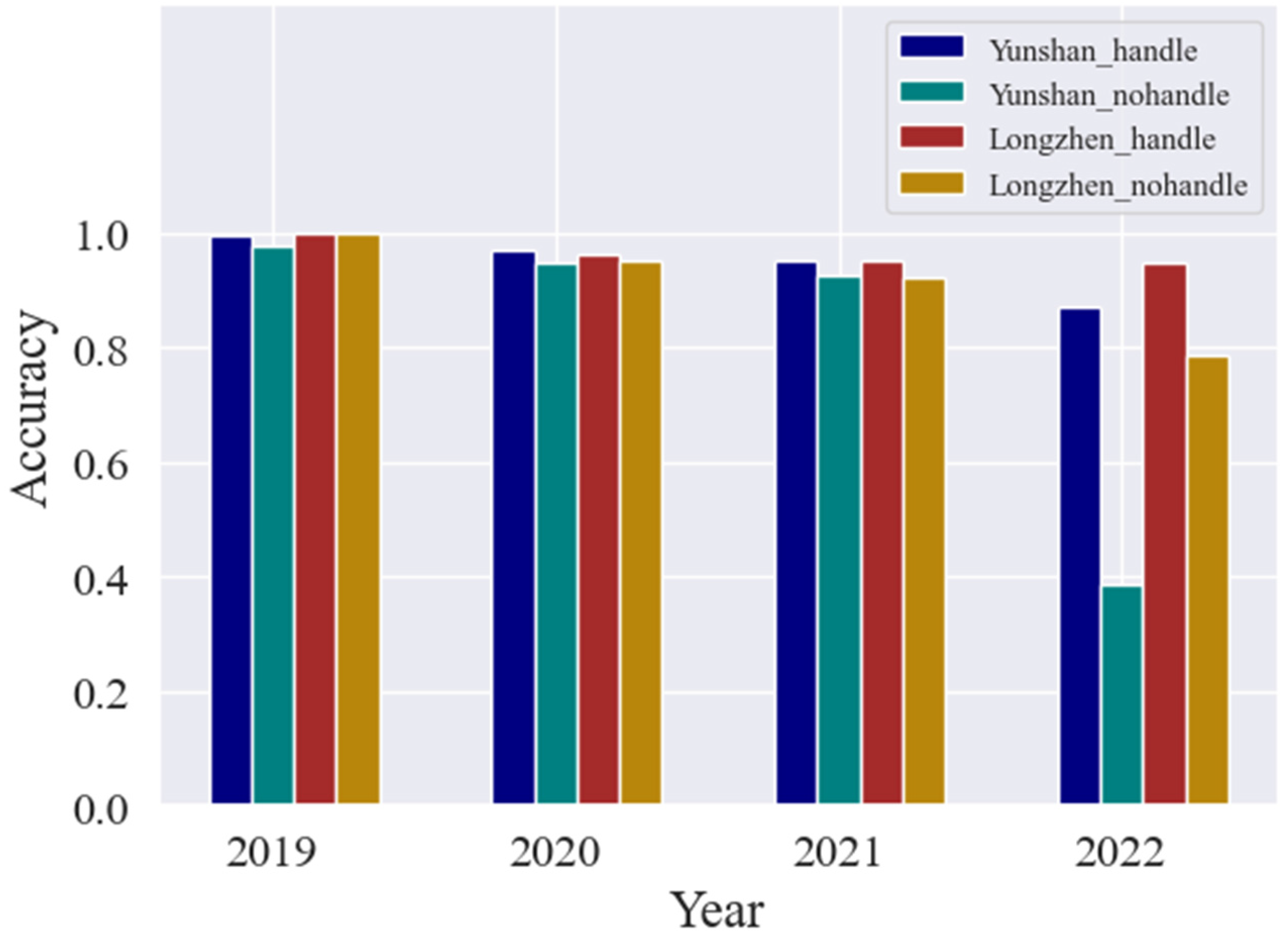
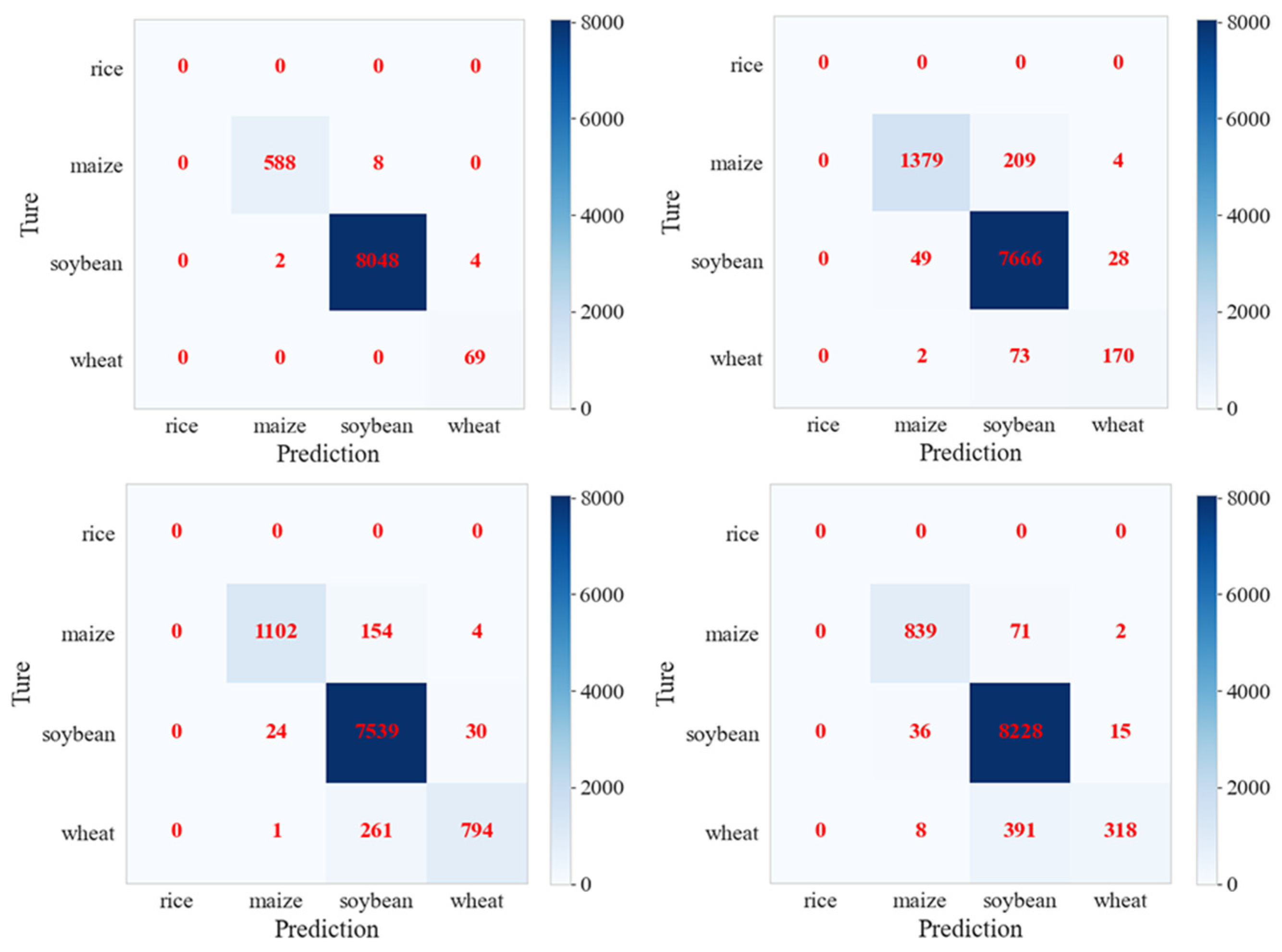
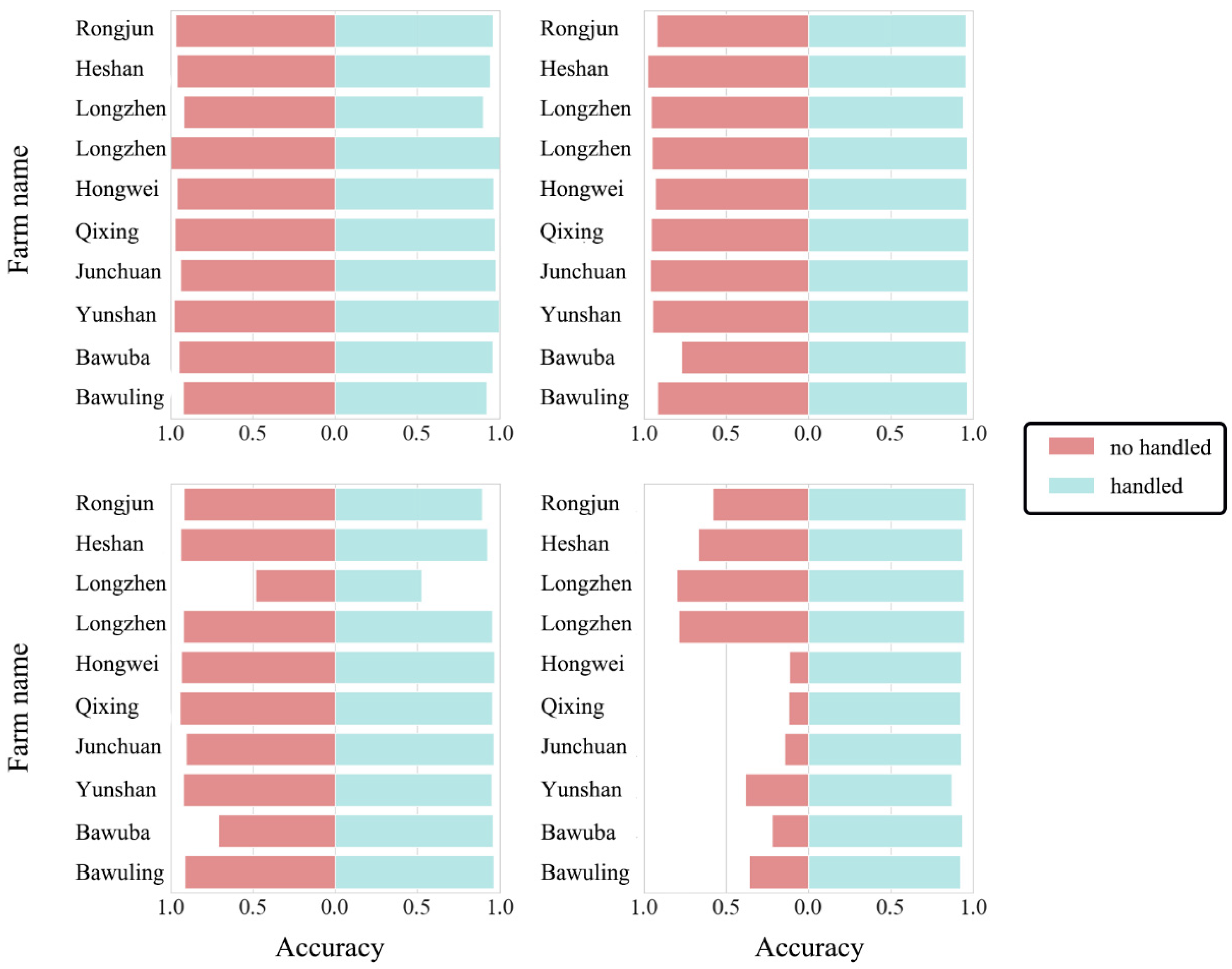
4.1. Comparison of the Improvement in Forecast Accuracy across Time Domains with the HTDM

The accuracy of random sampling points at Yunshan and Longzhen Farms from 2019 to 2022 has been evaluated by processing with the HTDM (Figure 4). The results without the HTDM for 2019 were considered as the training set accuracy. The results show that the training set accuracy for Yushan Farm is 97.65%, and for Longzhen Farm, it is 97.84%. Prediction accuracies for Yushan Farm for the years 2020 to 2022 are 94.90%, 92.50%, and 38.68%, respectively, while for Longzhen Farm, they are 95.72%, 89.60%, and 84.81%. From the training set results, it can be inferred that using HUNTS filtering to extract feature indices of each month as input features results in high training set accuracy, indicating that the feature extraction method captures time series features that effectively differentiate between crops. The results’ accuracy shows that compared to previous studies, which selected high-quality remote-sensing images and directly composed them into a time series by time, the filtering-based time series construction method used in this study, while retaining sufficient time series information, provides a feasible approach for creating simple, stable image datasets across different years.

There are certain differences in the imagery of various crops between years; these differences can lead to a decrease in prediction accuracy, with the lowest accuracy and largest classification difference due to image quality apparent in 2022. In the 2019 results, when the hypothesis testing distribution method was applied, there was a slight drop in the same year’s accuracy for both Yushan and Longzhen farms, possibly because the vegetation index features for crops in the same year already have certain differences between the farms. Combining datasets for correction could result in a decrease in classification accuracy. For cross-temporal prediction results, combining the previous conjectures on the modified classification accuracy after applying the hypothesis testing distribution method for the same year, the 2020 vegetation index features were close to the training set year, possessing high prediction accuracy before correction, and after applying the HTDM, accuracy might slightly decrease or increase. For 2022, due to the significant offset in vegetation index feature values, the prediction accuracies for Yushan and Longzhen farms without applying the HTDM are 38.69% and 84.82%, respectively, and after processing, they become 87.2% and 94.7%.

A comparison of crop accuracies before and after using the hypothesis testing distribution method reveals that when the inter-annual differences in image quality are small, the accuracies with the HTDM were close to the original ones. However, when there is a significant difference in image quality, applying the hypothesis testing distribution method can markedly improve crop classification accuracy. However, the primary aim of the HTDM was to improve accuracy by adjusting input feature values, not optimizing the model itself. Therefore, this method can be used in conjunction with other domain adaptation enhancement methods, such as cross-domain alignment modules and domain feature mapping to a common feature space [26].

As shown in

Table 2. Kappa indices for Yunshan and Longzhen Farms from 2019 to 2022.

Year	Farm Name	Kappa	Kappa of Rice	Kappa of Maize	Kappa of Soybeans	Kappa of Wheat
2019	Yunshan	0.958	0.998	0.987	0.989	-
2020	Yunshan	0.949	0.974	0.937	0.929	-
2021	Yunshan	0.917	0.963	0.905	0.864	-
2022	Yunshan	0.793	0.793	0.967	0.695	-
2019	Longzhen	0.989	-	0.991	0.989	0.972
2020	Longzhen	0.875	-	0.896	0.874	0.755
2021	Longzhen	0.868	-	0.913	0.860	0.827
2022	Longzhen	0.794	-	0.928	0.790	0.585

, the Kappa indices for Yunshan Farm from 2019 to 2022 were 0.958, 0.949, 0.917, and 0.793, respectively. The overall accuracy was relatively high, with the Kappa index for soybeans in 2021 slightly lower at 0.860, but the rest exceeded 0.9. In 2022, the Kappa values for rice, maize, and soybeans were 0.970, 0.649, and 0.695, respectively, with rice classification exhibiting the highest accuracy. There was a tendency for the soybean pixels to be confused with maize, with soybeans being more likely to be predicted as maize pixels (Figure 5). The limitation in the information provided by 10 m resolution multispectral images for maize identification suggests that achieving higher prediction accuracy may demand the use of texture features from high-resolution images [53]. The primary crops at Longzhen Farm are maize, soybeans, and wheat, with overall classification Kappa indices of 0.989, 0.875, 0.868, and 0.794 for the years 2019 to 2022, respectively. The general trend in Kappa variability is consistent with Yushan Farm, showing a proportional decline as the difference between years increases. In 2022, the Kappa indices for maize, soybeans, and wheat were 0.928, 0.790, and 0.585, respectively. It can be observed from the confusion matrix that wheat is more likely to be predicted as soybeans (Figure 6). In summary, using the hypothesis testing method to predict various crops has produced certain degrees of accuracy. As the years change and feature offsets caused by image quality differences increase, the accuracy using the HTDM significantly improves compared to not using the method.

4.2. Robustness of Hypothetical Distribution Test Method for Different Crop Distributions

The XGBoost model, trained using data from Yushan Farm and Longzhen Farm in 2019, was used to predict the crop types of the remaining farms for different years (Figure 7). In the figure, “handled” represents the result processed by the HTDM, while “no handled” represents the unprocessed results. Consistent with the hypothesis in Section 4.1, because image quality from 2020 to 2021 was similar to that of the training set, applying the HTDM did not significantly affect accuracy for most farms; with or without the method, accuracies remained at a relatively high level. However, the accuracies for the 858 farm prior to HTDM processing in 2020 and 2021 were 0.773 and 0.710, respectively, but after hypothesis testing, they improved to 0.955 and 0.960, leveling with other farms. In 2022, due to greater differences in image quality, the classification accuracies for all farms were low without applying the HTDM. Specifically, Rongjun, Heshan, Longzhen, and Longmen farms had accuracies of 0.581, 0.669, 0.800, and 0.788, respectively, without using the HTDM; while for Hongwei, Qixing, and Junchuan farms, the accuracies were 0.117, 0.121, and 0.148. The disparity in classification accuracies between the two groups of farms was mainly due to the actual distribution of crops, where the proportion of soybeans in the first four farms was greater than 0.5, whereas in the latter three farms, the proportion was less than 0.1. Since feature offsets caused by differences in image quality led to pixels shifting towards soybeans, the higher the proportion of soybeans on a farm, the higher the classification accuracy. After HTDM adjustment, accuracies for all farms increased to above 0.85. In conclusion, the hypothesis testing distribution method can reduce these discrepancies to improve classification accuracy when overall quality changes in images lead to shifts in crop input feature values compared to the training set. Moreover, this method still maintains robustness in diverse crop distributions across multiple farms and years.

There has been little discussion in other scholars’ cross-year predictions about methods to improve prediction accuracy from the data processing perspective [54]. In the research by Muhammad et al. [41], the EVI index was used to build a time series input, similar to this paper’s approach of using a time series of vegetation indices as inputs. The difference lies in using the lower-resolution MODIS dataset and constructing a single vegetation feature sequence, which contains less information. The study trained on multiple years’ data and validated the remaining year’s data, achieving cross-year accuracy rates from 74.4% to 81.9% without the use of other processing methods. In contrast, this study only used one year’s data for training and achieved accuracies over 87% across all farms and years after applying the HTDM, thereby avoiding the variability in vegetation features due to multi-year weather conditions mentioned by Muhammad et al. Likewise, Sonobe et al. [40] had an accuracy of 89.1% when using same-year data for training and validation, but the cross-year prediction accuracy dropped to 78%. After implementing the HTDM in 2022, this study was able to raise the lowest accuracy from 11.6% to 87.3%, demonstrating that the remote-sensing quality differences in this research area were greater than in the aforementioned study but could be overcome by adjusting the input features to enhance prediction accuracy.

4.3. SHAP Analysis

During the classification process, we extracted a total of 30 features from the vegetation indices for every 15th day from April to August (Figure 8). In the figure, the x-axis indicates the feature values of the selected features, the right y-axis displays the SHAP values of each sample for that feature, and the left y-axis represents the selected subsidiary features being analyzed for interactions with the primary feature. It is evident from the graph that features from August are of higher importance compared to other months, with four out of the top ten importance indices originating from August, while three features from July featured in the top ten importance indices. These results suggest that the further along in the growing season, the more pronounced the differences in vegetation indices between different crops become, which is consistent with the conclusions drawn by Vuolo et al. [55]. RNDVI and LSWI are the most critical variables, with these two accounting for seven out of the top ten variables.

Analyzing the contribution of features to the identification of each crop in detail, LSWI is identified as the most critical index for distinguishing rice. This is mainly because LSWI is an index highly sensitive to water bodies; hence, using LSWI, rice can be relatively easily differentiated from other dryland crops [56]. The LSWI value from May contributes the most significantly to identifying rice. This is due to the fact that by mid-May, the paddy fields are fully flooded, and since rice is in the earlier stages of its growth cycle at this time [57], there is minimal obstruction of the water surface by the leaf area, resulting in the greatest difference in the LSWI characteristic due to the presence of water. The distribution of SHAP values for individual features of corn and soybean are quite similar, mainly showing that the SHAP value proportions of rice and corn are more similar to each other compared to the other two crop types. For wheat, the most critical index is IRECI, with the IRECI feature from August having the most significant effect in identifying wheat.

A subset of features was selected to construct the SHAP dependency plots (Figure 9). As shown in Figure 9a–d, it is apparent that the SHAP dependency plot for LSWI in May shows low sample dispersion and a dense vertical distribution of samples. This implies that among the samples with the same feature value, there is a high similarity in the contribution rate of LSWI to the recognition of different crops. Figure 9a reveals a positive correlation between LSWI5 and LSWI8, indicating that for all crops, the LSWI distribution among samples does not significantly change over time. Moreover, lower LSWI values have negative SHAP values for rice, suggesting that higher LSWI values increase the probability of the crop being rice, whereas for other crops, a higher LSWI leads to lower SHAP values. This inverse trend in SHAP values makes LSWI especially effective in distinguishing rice from the other three crops. In Figure 9b,c, the trends of dependency plots of LSWI5 for the identification of corn and soybeans are similar.

According to the findings of LM Wang’s research, indices such as NDWI and NDVI have limited impact on improving the accuracy of identifying corn and soybeans [58]. The lower SHAP values for soybeans, combined with previous confusion matrix analysis results, indicate that soybeans are more likely to be misclassified as corn during the crop classification process. An analysis of interactions with other features shows that there is no significant correlation between LSWI and MSAVI, whereas a higher RNDVI8 contributes more to identifying a pixel as soybean with respect to LSWI5. Figure 9d depicts the LSWI6 dependency plot for corn identification. Compared to LSWI5, both dependency plots exhibit a similar distribution trend, but with greater sample dispersion, indicating that the stability of using this feature for crop identification begins to diminish. This suggests that using LSWI as an input feature makes it easier to distinguish between crops at an earlier stage. In Figure 9e, we ascertain that the highest SHAP value for identifying wheat is for the feature IRECI8. Additionally, higher RNDVI8 values tend to bring the sample SHAP values closer to one. Figure 9f presents the RNDVI8 dependency plot for corn, where IRECI8 and RNDVI8 have a positive correlation, and a smaller RNDVI8 leads to higher SHAP values, thus increasing the probability of predicting the sample as corn.

5. Conclusions

In this study, the Sentinel-2 remote-sensing imagery was selected, and time series were constructed by sequentially calculating vegetation indices such as LSWI and SAVI. Subsequently, the HUNTS filtering method was employed to remove cloud-cover-induced image artifacts. The crop classification datasets were compiled from 10 farms spanning the years 2019 to 2022, with major crop types including rice, corn, soybeans, and wheat. A portion of the 2019 dataset was utilized for model training, while data from other years and farms were used for model analysis and evaluation. For feature selection, mid-filtered vegetation indices from April to August of each year were chosen to ensure cloud-free feature extraction and consider temporal information.

After that, given significant variations in image quality, the study proposed the hypothesis testing distribution method. This method, based on adjusting the numerical distribution of the test set through the training set, first hypothesizes and verifies the distribution, employs gradient descent to adjust the hypothetical distribution, and finally predicts more reliable classification results using the modified test set. The results indicate that the hypothesis testing distribution method significantly improves crop classification accuracy in cases of large differences in image quality. Additionally, the method demonstrates significant effectiveness across different farms with varying crop distributions in different years. For instance, Farm 858 showed unprocessed accuracy of 77.3% and 71.0% in 2020 and 2021, respectively, which increased to 95.5% and 96.0% after applying the hypothesis testing method.

As this study represents the first attempt to apply an iterative optimization algorithm for remote-sensing crop image classification, and the selected sites are farms with relatively few crop types, the computational power requirements may increase when dealing with more complex crop types. Furthermore, the effectiveness of gradient-based decay distribution optimization during the iterative process remains to be further investigated. Additionally, the optimization logic of the hypothesis testing method proposed in this paper may not be perfect, as it relies on assumptions about crop distribution. Therefore, using this method for iterative optimization may lead to reduced loss rates but potentially large discrepancies between classification results and actual label values. While extreme cases did not occur in this paper’s results, addressing this issue will be a focus for future research optimization. In addition to the specific application, the HTDM can also be extended to other application scenarios. Since this method and model framework optimization, as well as input data design, are not within the same design phase, it can be combined with other optimization methods to improve cross-scale accuracy, thus maximizing improvement. The primary purpose of modifying input values is to address the issue of input data quality offsets, so this method may be applied to break down barriers between different satellite images, enabling the application of models based on one remote-sensing image to another satellite image.

References

1. Jiang, Y.; Lu, Z.; Li, S.; Lei, Y.; Chu, Q.; Yin, X.; Chen, F. Large-Scale and High-Resolution Crop Mapping in China Using Sentinel-2 Satellite Imagery. Agriculture 2020, 10, 433. [Google Scholar] [CrossRef]
2. Luo, N.; Meng, Q.; Feng, P.; Qu, Z.; Yu, Y.; Liu, D.L.; Müller, C.; Wang, P. China Can Be Self-Sufficient in Maize Production by 2030 with Optimal Crop Management. Nat. Commun. 2023, 14, 2637. [Google Scholar] [CrossRef]
3. Davis, K.F.; Rulli, M.C.; Seveso, A.; D’Odorico, P. Increased Food Production and Reduced Water Use through Optimized Crop Distribution. Nat. Geosci. 2017, 10, 919–924. [Google Scholar] [CrossRef]
4. Tittonell, P.; Shepherd, K.D.; Vanlauwe, B.; Giller, K.E. Unravelling the Effects of Soil and Crop Management on Maize Productivity in Smallholder Agricultural Systems of Western Kenya—An Application of Classification and Regression Tree Analysis. Agric. Ecosyst. Environ. 2008, 123, 137–150. [Google Scholar] [CrossRef]
5. Guo, W.; Fu, Y.; Ruan, B.; Ge, H.; Zhao, N. Agricultural Non-Point Source Pollution in the Yongding River Basin. Ecol. Indic. 2014, 36, 254–261. [Google Scholar] [CrossRef]
6. Sun, B.; Zhang, L.; Yang, L.; Zhang, F.; Norse, D.; Zhu, Z. Agricultural Non-Point Source Pollution in China: Causes and Mitigation Measures. Ambio 2012, 41, 370–379. [Google Scholar] [CrossRef]
7. Xie, W.; Zhu, A.; Ali, T.; Zhang, Z.; Chen, X.; Wu, F.; Huang, J.; Davis, K.F. Crop Switching Can Enhance Environmental Sustainability and Farmer Incomes in China. Nature 2023, 616, 300–305. [Google Scholar] [CrossRef]
8. You, N.; Dong, J.; Huang, J.; Du, G.; Zhang, G.; He, Y.; Yang, T.; Di, Y.; Xiao, X. The 10-m Crop Type Maps in Northeast China during 2017. Sci. Data 2021, 8, 41. [Google Scholar] [CrossRef]
9. Pereira, L.S.; Paredes, P.; Hunsaker, D.J.; López-Urrea, R.; Shad, Z.M. Standard Single and Basal Crop Coefficients for Field Crops. Updates and Advances to the FAO56 Crop Water Requirements Method. Agric. Water Manag. 2021, 243, 106466. [Google Scholar] [CrossRef]
10. Novotny, V. Water Quality: Prevention, Identification and Management of Diffuse Pollution; Van Nostrand-Reinhold Publishers: New York, NY, USA, 1994; ISBN 0-442-00559-8. [Google Scholar]
11. Sun, X.; Ritzema, H.; Huang, X.; Bai, X.; Hellegers, P. Assessment of Farmers’ Water and Fertilizer Practices and Perceptions in the North China Plain. Irrig. Drain. 2022, 71, 980–996. [Google Scholar] [CrossRef]
12. Karthikeyan, L.; Chawla, I.; Mishra, A.K. A Review of Remote Sensing Applications in Agriculture for Food Security: Crop Growth and Yield, Irrigation, and Crop Losses. J. Hydrol. 2020, 586, 124905. [Google Scholar] [CrossRef]
13. Vyas, S.; Dalhaus, T.; Kropff, M.; Aggarwal, P.; Meuwissen, M.P. Mapping Global Research on Agricultural Insurance. Environ. Res. Lett. 2021, 16, 103003. [Google Scholar] [CrossRef]
14. Cai, Y.; Guan, K.; Peng, J.; Wang, S.; Seifert, C.; Wardlow, B.; Li, Z. A High-Performance and in-Season Classification System of Field-Level Crop Types Using Time-Series Landsat Data and a Machine Learning Approach. Remote Sens. Environ. 2018, 210, 35–47. [Google Scholar] [CrossRef]
15. Mountrakis, G.; Im, J.; Ogole, C. Support Vector Machines in Remote Sensing: A Review. ISPRS J. Photogramm. Remote Sens. 2011, 66, 247–259. [Google Scholar] [CrossRef]
16. Conrad, C.; Colditz, R.R.; Dech, S.; Klein, D.; Vlek, P.L. Temporal Segmentation of MODIS Time Series for Improving Crop Classification in Central Asian Irrigation Systems. Int. J. Remote Sens. 2011, 32, 8763–8778. [Google Scholar] [CrossRef]
17. Tatsumi, K.; Yamashiki, Y.; Torres, M.A.C.; Taipe, C.L.R. Crop Classification of Upland Fields Using Random Forest of Time-Series Landsat 7 ETM+ Data. Comput. Electron. Agric. 2015, 115, 171–179. [Google Scholar] [CrossRef]
18. Fan, C.; Lu, R. UAV Image Crop Classification Based on Deep Learning with Spatial and Spectral Features. In Proceedings of the IOP Conference Series: Earth and Environmental Science, Zhangjiajie, China, 23–25 April 2021; IOP Publishing: Bristol, UK, 2021; Volume 783, p. 012080. [Google Scholar]
19. Yang, S.; Gu, L.; Li, X.; Jiang, T.; Ren, R. Crop Classification Method Based on Optimal Feature Selection and Hybrid CNN-RF Networks for Multi-Temporal Remote Sensing Imagery. Remote Sens. 2020, 12, 3119. [Google Scholar] [CrossRef]
20. Agilandeeswari, L.; Prabukumar, M.; Radhesyam, V.; Phaneendra, K.L.N.B.; Farhan, A. Crop Classification for Agricultural Applications in Hyperspectral Remote Sensing Images. Appl. Sci. 2022, 12, 1670. [Google Scholar] [CrossRef]
21. Chakhar, A.; Ortega-Terol, D.; Hernández-López, D.; Ballesteros, R.; Ortega, J.F.; Moreno, M.A. Assessing the Accuracy of Multiple Classification Algorithms for Crop Classification Using Landsat-8 and Sentinel-2 Data. Remote Sens. 2020, 12, 1735. [Google Scholar] [CrossRef]
22. Neetu; Ray, S.S. Exploring Machine Learning Classification Algorithms for Crop Classification Using Sentinel 2 Data. Int. Arch. Photogramm. Remote Sens. Spat. Inf. Sci. 2019, 42, 573–578. [Google Scholar]
23. Shi, M.; Xie, F.; Zi, Y.; Yin, J. Cloud Detection of Remote Sensing Images by Deep Learning. In Proceedings of the 2016 IEEE International Geoscience and Remote Sensing Symposium (IGARSS), Beijing, China, 10–15 July 2016; pp. 701–704. [Google Scholar]
24. Kussul, N.; Lavreniuk, M.; Skakun, S.; Shelestov, A. Deep Learning Classification of Land Cover and Crop Types Using Remote Sensing Data. IEEE Geosci. Remote Sens. Lett. 2017, 14, 778–782. [Google Scholar] [CrossRef]
25. Shen, H.; Li, H.; Qian, Y.; Zhang, L.; Yuan, Q. An Effective Thin Cloud Removal Procedure for Visible Remote Sensing Images. ISPRS J. Photogramm. Remote Sens. 2014, 96, 224–235. [Google Scholar] [CrossRef]
26. Lu, X.; Gong, T.; Zheng, X. Multisource Compensation Network for Remote Sensing Cross-Domain Scene Classification. IEEE Trans. Geosci. Remote Sens. 2020, 58, 2504–2515. [Google Scholar] [CrossRef]
27. Xu, L.; Zhang, H.; Wang, C.; Zhang, B.; Liu, M. Crop Classification Based on Temporal Information Using Sentinel-1 SAR Time-Series Data. Remote Sens. 2018, 11, 53. [Google Scholar] [CrossRef]
28. Chakhar, A.; Hernández-López, D.; Ballesteros, R.; Moreno, M.A. Improving the Accuracy of Multiple Algorithms for Crop Classification by Integrating Sentinel-1 Observations with Sentinel-2 Data. Remote Sens. 2021, 13, 243. [Google Scholar] [CrossRef]
29. Li, H.; Zhang, C.; Zhang, S.; Atkinson, P.M. Crop Classification from Full-Year Fully-Polarimetric L-Band UAVSAR Time-Series Using the Random Forest Algorithm. Int. J. Appl. Earth Obs. Geoinf. 2020, 87, 102032. [Google Scholar] [CrossRef]
30. Argenti, F.; Lapini, A.; Bianchi, T.; Alparone, L. A Tutorial on Speckle Reduction in Synthetic Aperture Radar Images. IEEE Geosci. Remote Sens. Mag. 2013, 1, 6–35. [Google Scholar] [CrossRef]
31. Joshi, N.; Baumann, M.; Ehammer, A.; Fensholt, R.; Grogan, K.; Hostert, P.; Jepsen, M.; Kuemmerle, T.; Meyfroidt, P.; Mitchard, E.; et al. A Review of the Application of Optical and Radar Remote Sensing Data Fusion to Land Use Mapping and Monitoring. Remote Sens. 2016, 8, 70. [Google Scholar] [CrossRef]
32. Ulaby, F.T.; Long, D.G.; Blackwell, W.; Elachi, C.; Zebker, H. Microwave Radar and Radiometric Remote Sensing; University of Michigan Press: Ann Arbor, MI, USA, 2015. [Google Scholar]
33. Kwak, G.-H.; Park, N.-W. Impact of Texture Information on Crop Classification with Machine Learning and UAV Images. Appl. Sci. 2019, 9, 643. [Google Scholar] [CrossRef]
34. Reedha, R.; Dericquebourg, E.; Canals, R.; Hafiane, A. Transformer Neural Network for Weed and Crop Classification of High Resolution UAV Images. Remote Sens. 2022, 14, 592. [Google Scholar] [CrossRef]
35. Bégué, A.; Arvor, D.; Bellon, B.; Betbeder, J.; De Abelleyra, D.; PD Ferraz, R.; Lebourgeois, V.; Lelong, C.; Simões, M.; Verón, S.R. Remote Sensing and Cropping Practices: A Review. Remote Sens. 2018, 10, 99. [Google Scholar] [CrossRef]
36. Li, J.; Shen, Y.; Yang, C. An Adversarial Generative Network for Crop Classification from Remote Sensing Timeseries Images. Remote Sens. 2021, 13, 65. [Google Scholar] [CrossRef]
37. Zhong, L.; Hu, L.; Zhou, H. Deep Learning Based Multi-Temporal Crop Classification. Remote Sens. Environ. 2019, 221, 430–443. [Google Scholar] [CrossRef]
38. Ji, S.; Zhang, C.; Xu, A.; Shi, Y.; Duan, Y. 3D Convolutional Neural Networks for Crop Classification with Multi-Temporal Remote Sensing Images. Remote Sens. 2018, 10, 75. [Google Scholar] [CrossRef]
39. Wang, Z.; Zhang, H.; He, W.; Zhang, L. Phenology Alignment Network: A Novel Framework for Cross-Regional Time Series Crop Classification. In Proceedings of the 2021 IEEE/CVF Conference on Computer Vision and Pattern Recognition Workshops (CVPRW), Nashville, TN, USA, 19–25 June 2021; pp. 2934–2943. [Google Scholar]
40. Sonobe, R.; Tani, H.; Wang, X.; Kobayashi, N.; Shimamura, H. Parameter Tuning in the Support Vector Machine and Random Forest and Their Performances in Cross- and Same-Year Crop Classification Using TerraSAR-X. Int. J. Remote Sens. 2014, 35, 7898–7909. [Google Scholar] [CrossRef]
41. Muhammad, S.; Zhan, Y.; Wang, L.; Hao, P.; Niu, Z. Major Crops Classification Using Time Series MODIS EVI with Adjacent Years of Ground Reference Data in the US State of Kansas. Optik 2016, 127, 1071–1077. [Google Scholar] [CrossRef]
42. Xue, J.; Su, B. Significant Remote Sensing Vegetation Indices: A Review of Developments and Applications. J. Sens. 2017, 2017, 1353691. [Google Scholar] [CrossRef]
43. Chandrasekar, K.; Sesha Sai, M.V.R.; Roy, P.S.; Dwevedi, R.S. Land Surface Water Index (LSWI) Response to Rainfall and NDVI Using the MODIS Vegetation Index Product. Int. J. Remote Sens. 2010, 31, 3987–4005. [Google Scholar] [CrossRef]
44. Li, H.; Shi, Q.; Wan, Y.; Shi, H.; Imin, B. Using Sentinel-2 Images to Map the Populus Euphratica Distribution Based on the Spectral Difference Acquired at the Key Phenological Stage. Forests 2021, 12, 147. [Google Scholar] [CrossRef]
45. Wang, Z.; Zheng, Y.-C.; Li, J.-F.; Wang, Y.-Z.; Rong, L.-S.; Wang, J.-X.; Jiang, D.-C.; Qi, W.-C. Study on GLI Values of Polygonatum Odoratum Base on Multi-Temporal of Unmanned Aerial Vehicle Remote Sensing. Zhongguo Zhong Yao Za Zhi Zhongguo Zhongyao Zazhi China J. Chin. Mater. Medica 2020, 45, 5663–5668. [Google Scholar]
46. Chen, J.; Jönsson, P.; Tamura, M.; Gu, Z.; Matsushita, B.; Eklundh, L. A Simple Method for Reconstructing a High-Quality NDVI Time-Series Data Set Based on the Savitzky–Golay Filter. Remote Sens. Environ. 2004, 91, 332–344. [Google Scholar] [CrossRef]
47. Chen, T.; Guestrin, C. Xgboost: A Scalable Tree Boosting System. arXiv 2016, arXiv:1603.02754. [Google Scholar]
48. Mousa, S.R.; Bakhit, P.R.; Ishak, S. An Extreme Gradient Boosting Method for Identifying the Factors Contributing to Crash/near-Crash Events: A Naturalistic Driving Study. Can. J. Civ. Eng. 2019, 46, 712–721. [Google Scholar] [CrossRef]
49. Zhang, J. Gradient Descent Based Optimization Algorithms for Deep Learning Models Training. arXiv 2019, arXiv:1903.03614. [Google Scholar]
50. Chmura Kraemer, H.; Periyakoil, V.S.; Noda, A. Kappa Coefficients in Medical Research. Stat. Med. 2002, 21, 2109–2129. [Google Scholar] [CrossRef] [PubMed]
51. Cohen, J. A Coefficient of Agreement for Nominal Scales. Educ. Psychol. Meas. 1960, 20, 37–46. [Google Scholar] [CrossRef]
52. Lundberg, S.M.; Lee, S.-I. A Unified Approach to Interpreting Model Predictions. arXiv 2017, arXiv:1705.07874. [Google Scholar]
53. Iqbal, N.; Mumtaz, R.; Shafi, U.; Zaidi, S.M.H. Gray Level Co-Occurrence Matrix (GLCM) Texture Based Crop Classification Using Low Altitude Remote Sensing Platforms. PeerJ Comput. Sci. 2021, 7, e536. [Google Scholar] [CrossRef]
54. Chong, K.L.; Lai, S.H.; Ahmed, A.N.; Zaafar, W.Z.W.; Rao, R.V.; Sherif, M.; Sefelnasr, A.; El-Shafie, A. Review on Dam and Reservoir Optimal Operation for Irrigation and Hydropower Energy Generation Utilizing Meta-Heuristic Algorithms. IEEE Access 2021, 9, 19488–19505. [Google Scholar] [CrossRef]
55. Vuolo, F.; Neuwirth, M.; Immitzer, M.; Atzberger, C.; Ng, W.-T. How Much Does Multi-Temporal Sentinel-2 Data Improve Crop Type Classification? Int. J. Appl. Earth Obs. Geoinf. 2018, 72, 122–130. [Google Scholar] [CrossRef]
56. Xiang, K.; Yuan, W.; Wang, L.; Deng, Y. An LSWI-Based Method for Mapping Irrigated Areas in China Using Moderate-Resolution Satellite Data. Remote Sens. 2020, 12, 4181. [Google Scholar] [CrossRef]
57. Owusu-Mensah, E.; Oduro, I.; Sarfo, K.J. Steeping: A way of improving the malting of rice grain: Improving the malting of rice grain. J. Food Biochem. 2011, 35, 80–91. [Google Scholar] [CrossRef]
58. Wang, L.; Liu, J.; Yang, L.; Yang, F.; Fu, C. Application of Random Forest Method in Maize-Soybean Accurate Identification. Acta Agron. Sin. 2018, 44, 569–580. [Google Scholar] [CrossRef]
Figure 1. Distribution map of farms in the research area.
Agronomy 14 01084 g001
Figure 2. Mean NDVI time series for Yunshan Farm for the years 2019–2022.
Agronomy 14 01084 g002
Figure 3. HTDM iteration flowchart.
Agronomy 14 01084 g003
Figure 4. Accuracy comparison of Yushan Farm and Longzhen Farm from 2019 to 2022 utilizing the HTDM.
Agronomy 14 01084 g004
Figure 5. Confusion matrix of annual classification results for Yunshan Farm from 2019 to 2022. The x-axis represents the classification results obtained after model prediction, and the y-axis represents the labels of the samples.
Agronomy 14 01084 g005
Figure 6. Confusion matrix of annual classification results for Longzhen Farm from 2019 to 2022.
Agronomy 14 01084 g006
Figure 7. Accuracy of classification results using the hypothesis testing distribution method among farms from 2019 to 2022.
Agronomy 14 01084 g007
Figure 8. SHAP summary plot.
Agronomy 14 01084 g008
Figure 9. SHAP dependency analysis. The x-axis indicates the feature values of the selected features, the right y-axis displays the SHAP values of each sample for that feature, and the left y-axis represents the selected subsidiary features being analyzed for interactions with the primary feature.
Agronomy 14 01084 g009