Rapid pH Value Detection in Secondary Fermentation of Maize Silage Using Hyperspectral Imaging

Abstract

As pH is a key factor affecting the quality of maize silage, its accurate detection is essential to ensuring product quality. Although traditional methods for testing the pH of maize silage feed are widely used, the procedures are often complex and time-consuming and may damage the sample. This study presents a non-destructive hyperspectral imaging (HSI) technology that provides a more efficient and cost-effective method of monitoring pH by capturing the spectral information of samples and analyzing their chemical and physical properties rapidly and without contact. We applied four spectral preprocessing methods, among which the multiplicative scatter correction (MSC) preprocessing method yielded the best results. To minimize model redundancy and enhance predictive performance, we utilized six feature extraction methods for characteristic wavelength extraction, integrating these with partial least squares (PLS), non-linear support vector machine regression (SVR), and extreme learning machine (ELM) algorithms to construct a quantitative pH value prediction model. The results showed that the model based on the bootstrapping soft shrinkage (BOSS) feature wavelength extraction method outperformed the other feature extraction methods, selecting 20 pH value-related feature wavelengths from 256 bands and building a stable BOSS–ELM model with prediction set determination coefficient $(R_P^2$), root-mean-square error of prediction (RMSEP), and relative percentage deviation (RPD) values of 0.9241, 0.4372, and 3.6565, respectively. To further optimize the model for precisely predicting pH at each pixel in hyperspectral images, we employed three algorithms: the genetic algorithm (GA), whale optimization algorithm (WOA), and bald eagle search (BES). These algorithms optimized and compared the BOSS–ELM model to obtain the best model for predicting maize silage pH: the BOSS–BES–ELM model. This model achieved a determination coefficient ($R_P^2)$ of 0.9598, an RMSEP of 0.3216, and an RPD of 5.1448. We generated a visualized distribution map of pH value variation in maize silage using the BOSS–BES–ELM model. This study provides strong technical support and a reference for the rapid, non-destructive detection of maize silage pH from an image, an advancement of great significance to ensuring the quality of maize silage.

1. Introduction

Maize silage is a nutrient-rich feed made from the above-ground portion of maize harvested from its late-milk stage to its waxy mature stage; the maize is crushed, cut short, processed, sealed, stored, and fermented [1]. Maize silage has become an important source of roughage for ruminants globally due to its nutritional richness, good palatability, high digestibility, and long shelf life. It is also an exemplary feed for the development of animal husbandry in China [2,3].

The production of maize forage silage is divided into the following four main phases: (1) an aerobic phase in which the maize is placed in a closed environment after it is harvested, (2) fermentation, (3) stabilization and storage, and (4) exposure to air after the silage is unsealed and removed [4,5]. Currently, during the fourth stage of the silage production process, unavoidable exposure to air while removing the feed brings it into contact with oxygen. This leads to secondary fermentation, resulting in a gradual deterioration in feed quality which impacts ruminant intake and feeding safety [6]. pH is a key indicator when evaluating secondary fermentation quality, and quality maize silage should have a pH value between 3.7 and 4.0 [7]. Moreover, a suitable pH aids in the growth of beneficial flora and inhibits the growth of harmful microorganisms. Reasonable pH control is essential to ensuring maize silage quality and shelf life. Currently, pH detection in maize silage is mainly based on the laboratory method, which is accurate but requires the destruction of samples, is time-consuming and expensive, and cannot satisfy the need to rapidly evaluate pH at the production site. Therefore, at livestock breeding production sites, sensors are used to achieve rapid, scientific evaluations of maize silage quality instead of cumbersome laboratory testing, demonstrating an inevitable development trend.

In recent years, near-infrared (NIR) spectroscopy has demonstrated its potential for use in quantitative information analyses in the field of non-destructive maize silage testing. Due to different chemical compositions and physical structures within each sample, they reflect, scatter, absorb, and emit electromagnetic energy in different ways at specific wavelengths when examined using NIR spectroscopy [8]. For example, Sørensen et al. [9] used NIR spectroscopy to predict fermentation quality indicators for dry and wet samples of maize silage forage; the model’s prediction correlation coefficients for pH were 0.78 and 0.62 for the dry and wet samples, respectively. Liu et al. [10] used a combination of near-infrared spectroscopy in the 1000–2500 nm range and partial least squares (PLS) regression to develop a quantitative model for analyzing the fermentation and nutritional indexes of maize silage. Cozzolino et al. [11] used visible (VIS) and near-infrared reflectance (NIR) spectroscopy to examine nutrient indicators and pH in wet maize silage samples, and they developed predictive equations using various preprocessing methods and the modified partial least squares (MPLS) method. The results showed a correlation coefficient of 0.6 for the model’s pH value predictions. Zhang et al. [12] used NIR spectroscopy to determine the moisture of maize silage stover forage by comparing the raw spectra results of five preprocessing methods and establishing a modified partial least squares (MPLS) regression quantification model. The results showed that the correlation coefficient of the calibration set model established via the use of successive preprocessing multiplicative scatter correction (MSC) and the first derivative was 0.9740. However, the NIR spectroscopy technique has limitations as acquisition comprises a single-point measurement, providing limited data on the range of samples collected which are not representative of the entire sample. Therefore, researchers have combined spectroscopic techniques with imaging techniques to develop hyperspectral imaging (HSI).

HSI can obtain two-dimensional image information and one-dimensional spectral information from an object without damaging the sample. The acquired hyperspectral image is a data cube that contains the external physical and internal chemical characteristics of the sample, enabling the effective measurement of non-uniform samples [13,14]. In recent years, HSI has been widely used for internal quality inspections of agricultural products. Hu et al. [15] used HSI to determine levels of tea polyphenols and free amino acids by combining multiple preprocessing methods with machine learning (ML), and an analysis of their results showed that SG-SNV-PCA-Extratree’s prediction accuracy ($R_P^2)$ for tea polyphenols was 0.9248, and the precision ${(R}_P^2)$ of SG-MSC-PCA-Extratree‘s prediction of free amino acids was 0.8736. Wang et al. [16] took a maize single seed as their research object, acquired hyperspectral images of it in the wavelength range of 930–2548 nm, proposed a combination of competitive adaptive reweighted sampling (CARS) and the successive projections algorithm (SPA), and extracted the feature bands, which were modelled using the PLSR and least squares support vector machine (LS-SVM) methods, respectively. The results showed that the accuracy of the moisture prediction model and the RMSEP established by the CARS-SPA-LS-SVM method were 0.9311 and 1.2131, respectively. Yu et al. [17] utilized HSI and time-series phenotyping to predict the soluble solids content (SSC), pH value, nitrate (${\mathrm{N}\mathrm{O}}_3^{-}$) content, and calcium (Ca²⁺) content of lettuce under water stress; the results showed that the Inception-residual-TD model was optimal for predicting pH, with an $R_P^2$ of 0.9583. Yao et al. [18] developed a portable hyperspectral scanner that quantitatively predicted the pH of meat samples using spectral reflectance and non-linear support vector machine regression (SVR) modelling to an accuracy of about 0.90. Ma et al. [19] designed a push-broom-type NIR imaging system and rotationally scanned the entire surface of a kiwifruit. Then, characteristic wavelengths in the range of 1002–2300 nm were extracted via a partial least squares regression analysis to construct SSC and pH value calibration models; for the SSC, the prediction set coefficient of determination (${\mathrm{R}}_{\mathrm{C}\mathrm{V}}^2$) was 0.74, and for pH, the prediction set coefficient of determination (${\mathrm{R}}_{\mathrm{C}\mathrm{V}}^2$) was 0.64. Finally, the SSC and pH were visualized. It is clear from the literature that the application of HSI is mainly focused on food and agricultural products, and fewer studies have been conducted on the pH of maize silage.

This study aims to develop a fast and non-destructive method of detecting the pH of maize silage based on HSI to realize fast, convenient, and real-time pH index monitoring during the secondary fermentation of maize silage to ensure its quality. The main objectives of this study are as follows: (1) to explore the feasibility of using HSI to quantitatively analyze the pH of maize silage; (2) to use six feature wavelength selection methods to determine feature wavelengths related to the pH value and model them using SVR, PLS, and extreme learning machine (ELM) algorithms to determine a stable quantitative prediction model; (3) to use different optimization algorithms to optimize the stable prediction model, compare its performance following optimization, and select an optimal quantitative prediction model for the pH value of maize silage; and (4) to establish a visualization of pH distribution during the secondary fermentation of maize silage.

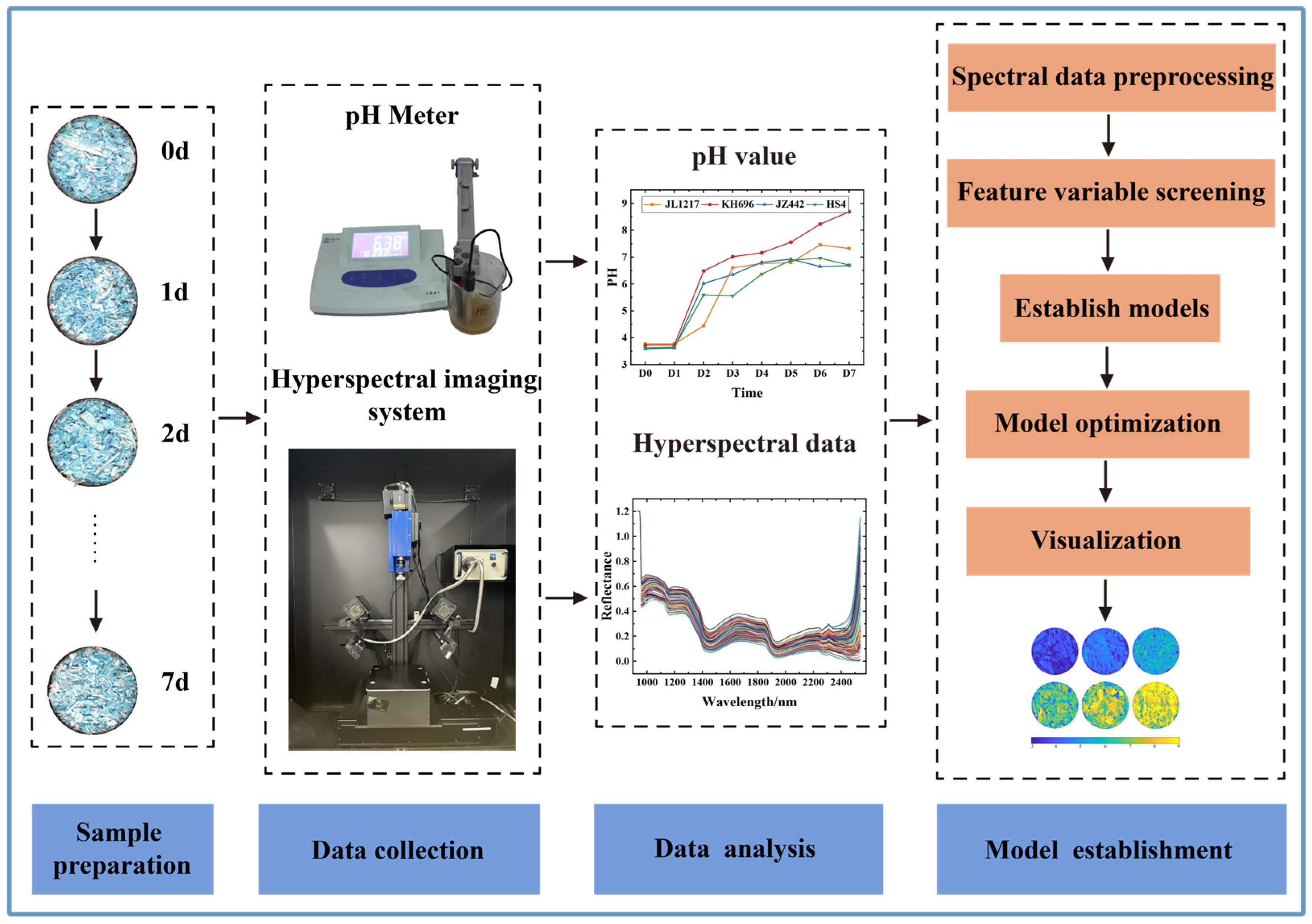
2. Materials and Methods

2.1. Sample Preparation

This experiment was conducted from July 2023 to October 2023. Samples of maize silfage that had been stored for eight months or more were purchased in four batches. The origins, varieties, and methods of storing the samples were as follows: (1) the maize varieties from Donghuaying Village, Tuzuo Banner, Hohhot City, Inner Mongolia, China (111°58′ E, 40°58′ N), were Long 1217 (stored in a glass jar) and Kehe 696 (stored in a cellar); (2) the maize silage varieties from Taihe County, Fuyang City, Anhui Province, China (115°80′ E, 33°38′ N), were Jingza442 and Hongsai4, and both were stored using the film-wrapping method.

The maize silage samples used in the experiment were sealed in special silage bags and transported at a low temperature. Each batch of samples was mixed immediately after its transportation to the laboratory. Each batch of maize silage was divided into sixteen 4 kg portions which were placed in polystyrene boxes according to the quadrat method [6], pressed firmly, and covered with tin foil (the dimensions of the polystyrene boxes were 500 mm × 365 mm × 265 mm, and the maize silage samples in the boxes were about 60 mm thick). On days 0–7 of the experiment, we treated the collected samples with continuous aerobic exposure. Specifically, from day 0 to day 7 of the experiment, we sampled maize silage from each of two randomly selected polystyrene boxes three times per day, with each sampling including a sample randomly selected from the box for a total of six samples analyzed per day. All samples were processed in an indoor environment at 20–24 °C. Over the course of the experiment, we collected a total of 192 samples which were subjected to hyperspectral imaging acquisition and pH value determination. The test and data analysis processes are shown in Figure 1.

2.2. Hyperspectral Imaging System and Image Acquisition

The hyperspectral imaging system utilized in this experiment was acquired from ISUZU Optics Co., Ltd., Taiwan, China. The system comprises several key components: a hyperspectral image spectrometer (ImSpector Model N25E, Spectral Imaging Ltd., Oulu, Finland), a CCD camera (Xeva-FPA-2.5-320, Xenics Ltd., Leuven, Belgium), six halogen lamps (for three 50 W lamps per group) (DECOSTAR^® 51 STANDARD, OSRAM Ltd., Munich, Germany), a mobile control platform (IRCP0076-1COM, ISUZU Optics Co., Ltd., Taiwan, China), and a computer.

The hyperspectral imaging system had a spectral range of 935–2539 nm, a resolution of 8 nm, and a total of 256 bands. The optimal parameters were derived from the pre-experiment: the distance between the sample and the lens was 455 mm, the moving platform moved at 20.38 mm/s during the acquisition process, the exposure time was 2.16 ms, and the actual length and width of the area to be scanned were 180 mm and 80 mm, respectively. Each sample weighed 50 ± 0.5 g, and samples were evenly distributed in culture dishes (Φ × h: 10 cm × 1 cm).

In order to reduce the effect of the dark current and light intensity of the instrument on the spectral image during the acquisition process, we corrected the original hyperspectral images with white and dark references, using the following correction equation [20,21]:

$$R=\frac{I_S-I_D}{I_W-I_D}$$

(1)

where $R$ is the black-and-white corrected sample image; $I_S$ is the original image of the sample; $I_D$ is a dark reference image obtained with the optical lens cover covering the optical lens after turning off the lamp; and $I_W$ is a reference image obtained from a standard calibrated whiteboard with 99% reflectivity.

2.3. HSI Data Extraction

Feature extraction from the acquired hyperspectral images was carried out using ENVI5.3 software (ITT Visual Information Solutions, Boulder, CO, USA), avoiding the reflective and shadowed parts when selecting the region of interest (ROI). Given that the maize silage samples contained multiple parts of the plant and were heterogeneous, when selecting regions of interest (ROIs), we included representative parts of the whole maize plant, such as old leaves, new leaves, young leaves, stover bark, chopped stover, and kernels; therefore, two 15 × 15-pixel rectangular areas were manually selected as regions of interest (ROI) for each representative part. A total of 12 ROIs were selected for each image. Finally, the spectral data of all pixels within each ROI were extracted, the average spectrum was calculated as a representative spectrum for this sample, and 192 pieces of spectral data were obtained.

2.4. pH Measurement

The pH of the maize silage was determined according to the Chinese national standard method (GB 5009.237-2016) [22] and the local standard method (DB15/T 1458-2018) [23]. At room temperature (temperature: 24–26 °C; humidity: 25%), using the quartering method, each sample was reduced to 10 g (±0.01 g) and placed in a beaker, mixed with 90 mL of distilled water, and allowed to stand for 30 min [6]. The extracts were filtered through four layers of gauze and measured using a pH value meter (PHS-3CB, Shanghai Yue Ping Scientific Instrument Co., Ltd., Shanghai, China) with a resolution of 0.01 and an accuracy of ±0.01. Measurements were repeated five times for each sample, and the results were taken as the arithmetic mean.

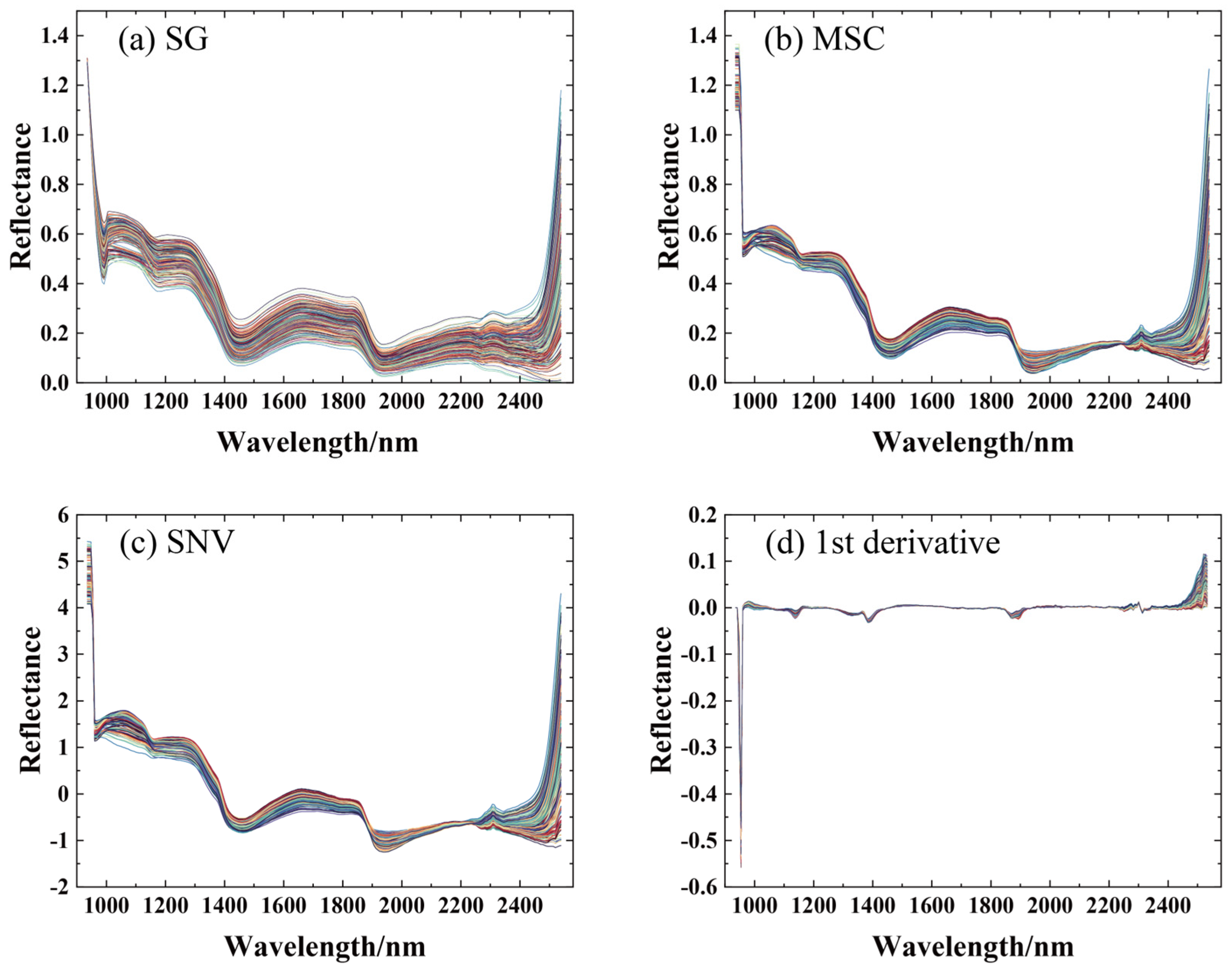
2.5. Spectral Data Preprocessing

The surface of the maize silage is not flat; this irregularity causes its spectral information to be affected by light scattering. In addition, instrumental noise and dark current will also affect the spectral information, so a spectral preprocessing method is needed to eliminate sample-independent information in order to improve the accuracy of the model’s predictions [24]. In this study, four methods, Savitzky–Golay (SG) smoothing, multiplicative scatter correction (MSC), the standard normal variate (SNV) method, and the first derivative method (1st derivative), were used to preprocess the spectral data. SG smoothing can smooth out the noise in a spectrum [25]; the 1st derivative eliminates instrument-induced signal drift and improves the stability of the spectral curve [26]; the SNV method eliminates the effects of diffuse reflection due to solid particle size, surface scattering [27], and changes in the optical range; and MSC is mainly used to eliminate the scattering phenomenon caused by uneven particle distribution and particle size [28].

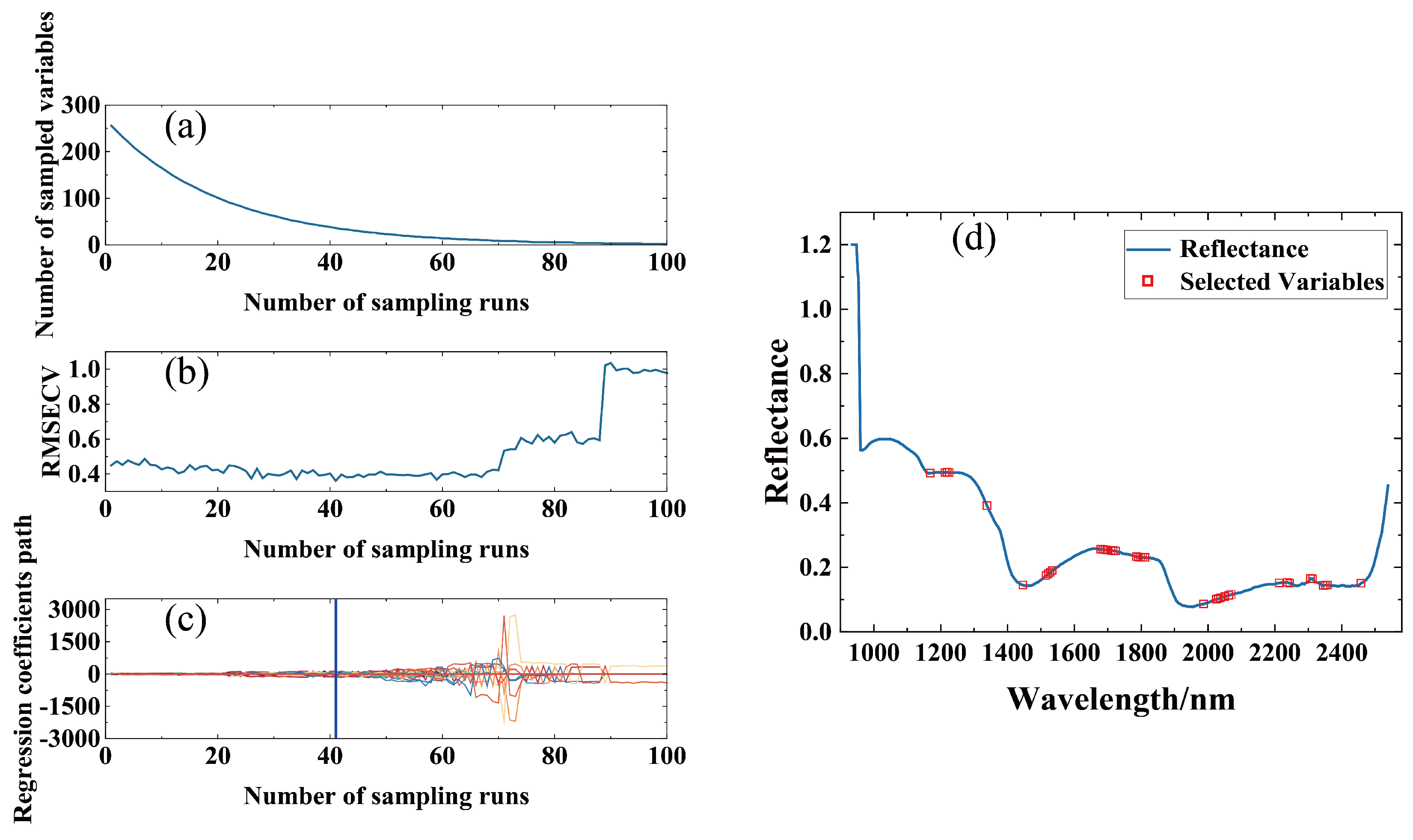
2.6. Feature Variable Screening

Hyperspectral data contain a large amount of redundant information unrelated to pH, which is detrimental to model building and affects the speed of model computation; therefore, this study utilized six feature band extraction methods to eliminate irrelevant information and simplify the model’s complexity.

The competitive adaptive reweighted sampling (CARS) algorithm is a feature selection method that combines the partial least squares (PLS) and Monte Carlo uninformative (MCU) variable elimination techniques. It is widely used in the field of spectral analysis. The method first selects a subset of N variables (comprising 80% of the calibration set) via multiple Monte Carlo sampling. The wavelengths are randomly selected for each sample, and the prediction performance is evaluated using a PLS model. The frequency of wavelength selection is recorded via adaptive reweighted sampling (ARS), and wavelengths with higher frequencies are considered more important. In each iteration, low contribution wavelengths are eliminated using an exponential decay function (EDF), and weights are redistributed. Eventually, a subset of PLS model wavelengths determined by the root mean square error of minimum cross-validation (RMSECV) is selected as the feature wavelengths [29].

Like the CARS algorithm, the successive projections algorithm (SPA) is widely used in spectral analysis. The algorithm starts with a single wavelength and constructs the wavelength set step by step. In each iteration, the SPA evaluates the orthogonal projection of each wavelength in the candidate wavelength set to the currently selected wavelength set. By calculating the projection error between the candidate wavelengths and the selected wavelengths, the wavelength that minimizes the overall model error is selected. This process continues until the number of selected wavelengths reaches a set value N or the addition of new wavelengths no longer significantly improves the model’s prediction performance [30].

The discrete wavelet transform (DWT) is used in the extraction of spectral data; the first wavelet decomposition of the spectrum (wavelet basis function db4 was used in this study) is used to obtain the spectrum’s high-frequency and low-frequency signals, and a singular value decomposition is carried out on the high-frequency portion. The wavelength corresponding to the larger singular value is extracted as the characteristic wavelength. To determine the characteristic wavelengths, the approximate components of the signal at the characteristic wavelength (the low-frequency part) obtained via selective decomposition are used as a spectral dataset for modelling at the characteristic wavelengths [31]. A hybrid algorithm combining the variable combination population analysis and iterative retained information variable (VCPA-IRIV) algorithms can compensate for the VCPA algorithm’s disadvantages in eliminating too many variables and the IRIV’s disadvantages in calculating the redundancy of variables, giving full play to the advantages of both. First, the variables are screened using the VCPA algorithm, after which the IRIV algorithm calculates the importance of the screened variables; finally, the best variables are indicated [32]. At the core of uninformative variable elimination (UVE) is utilizing the statistics of the irrelevant variable information of noise to select the characteristic variables of the spectrum itself. After adding noise, UVE will judge the variables according to the statistical distribution of the regression coefficients of the target matrix, which is composed of an independent variable matrix of spectral variables and noise in which the statistical distribution of the regression coefficients is expressed as the ratio of the mean and standard deviation values; it ultimately determines the characteristic variables by identifying the upper and lower bounds and proposing variables which fall in the corresponding ranges [33]. Bootstrapping soft shrinkage (BOSS) is a spectral feature extraction method proposed by Baichuan Deng in 2016 which is based on autonomous sampling (bootstrapping sampling, BSS) and weighted autonomous sampling (weighted bootstrap sampling, WBS). It applies BSS and WBS to generate submodels based on the weights of variables. It is characterized by the fact that during optimization, unimportant variables are assigned very low weights and are not removed [34].

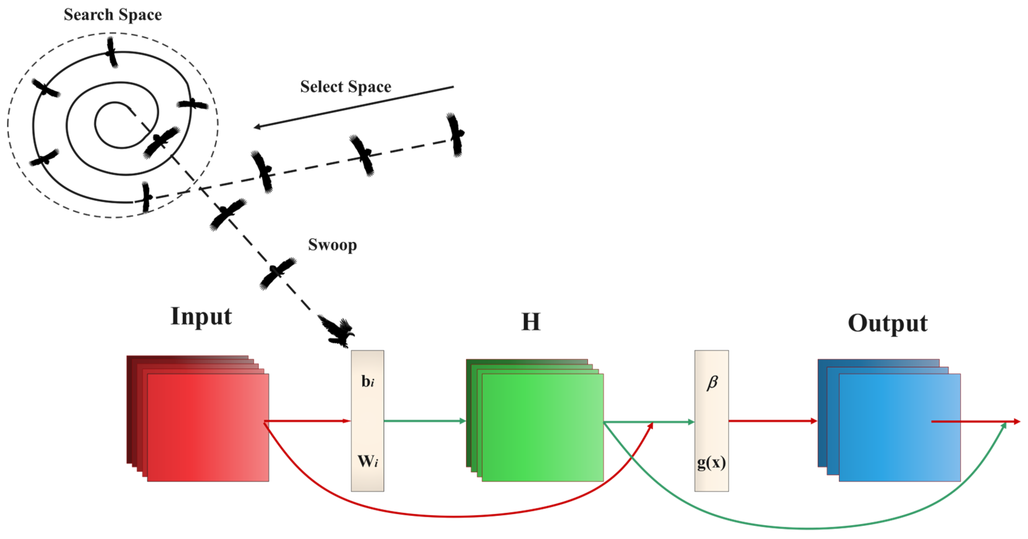
2.7. Establishment and Assessment of Models

In this study, three prediction models, the partial least squares (PLS), non-linear support vector machine regression (SVR), and extreme learning machine (ELM) models, were established to explore the relationship between feature spectral data and maize silage pH value and determine an optimal prediction model.

The PLS method is one of the most classical modelling approaches, and its core concept is to project the original explanatory and response variables into a new space and find the direction in this space that maximizes the covariance of the explanatory and response variables. In this way, the PLS method not only extracts important information for use in forecasting but also handles complex relationships and covariances between variables. The PLS method does so by extracting new variables called components (or latent variables and factors) which are linear combinations of the original explanatory variables. These components are constructed to maximize the covariance between explanatory and response variables. In practice, it is common to assess the impact of models containing different numbers of latent variables (LVs) on predictive performance through cross-validation methods to determine the number of LVs [35].

SVR is a regression model based on the classical support vector machine (SVM) algorithm which searches for an optimal regression hyperplane by mapping original data into a high-dimensional space. In addition, SVR introduces a regularization parameter c which is used to regulate the complexity and fault tolerance of the model, thus achieving a balance between its predictive accuracy and complexity. In this study, the radial basis function (RBF) was chosen as a kernel function, and in the application of the RBF kernel, the parameter g determined the distribution of data in the new space after mapping; in turn, this affected the decision boundary of the nonlinear SVR model [36].

The ELM is a special single-hidden-layer feedforward neural network model proposed by Prof. Guangbin Huang in 2004. The model includes an input layer, hidden layer, and output layer. In an ELM, the weights (W) and biases (b) of the input layer with respect to the hidden layer are randomly generated during the initialization of the model, while the weights of the output layer are directly computed via the parsing method. This computation makes use of the Moore–Penrose (MP) generalized inverse matrix, which is accomplished by minimizing a nonlinear combinatorial loss function containing the training error term and the output layer weight paradigm, thus eliminating the need to iteratively update the weights and biases of the hidden layer. The key to achieving success with the model is to set the right number of hidden layer neurons, which can ensure that the desired performance is achieved. Compared to traditional artificial neural networks, the ELM has significant advantages in terms of learning speed, generalization ability, and robustness [37,38]. The parameters and ranges of each model are shown in

Table 1. Parameters of each model.

Model	Row	Model Parameters	Values and Specifications
PLS	1	F	1–10
SVR	1	c	2−10–210 (value every 20.5)
	2	g	2−10–210 (value every 20.5)
ELM	1	W	−1–1
	2	b	0–1

.

The ELM model was optimized by comparing the models built at a later stage. We chose three optimization algorithms: the genetic algorithm (GA), whale optimization algorithm (WOA), and bald eagle search (BES). The GA is a classical optimization algorithm that simulates natural evolution and genetic theory to obtain a globally optimal solution as a search algorithm [39]. The WOA is a nature-inspired optimization algorithm proposed by Mirjalili scholars in 2016 that simulates the hunting and social behavior of whales, and it has the advantage of a fast search speed and global search capability [40]. The BES algorithm is a meta-heuristic optimization algorithm that mimics the foraging behavior of bald eagles. The BES algorithm draws on this behavioral pattern by dynamically updating the positions of “bald eagle” agents to find an optimization solution. As shown in Figure 2, the specific steps of the optimization of the ELM model are as follows [41]:

Step 1: Initialize the number of populations and iterations in the BES and the weights W and threshold b in the ELM.

Step 2: Generate an initial population with the location of each bald eagle corresponding to a randomly generated set of ELM parameters.

Step 3: Evaluate the performance of each bald eagle using the calibration set’s mean square error (MSE) as the objective function, and select the position of the bald eagle with the smallest MSE value as the current optimal solution.

Step 4: The other “bald eagles” update their positions according to the position of the optimal solution, and this process mimics the swooping behavior of the bald eagle.

Step 5: Perform steps 3 and 4 continuously until the set maximum number of iterations is satisfied.

In this study, the coefficient of determination for the calibration set ($R_C^2$), the root-mean-square error of calibration (RMSEC), the coefficient of determination for the prediction set ($R_P^2$), the root-mean-square error of prediction (RMSEP), and the relative percentage deviation (RPD) were used to evaluate the prediction accuracy and stability of each model. When the RPD value was greater than 2, it indicated that the model had high stability. In addition, each model was run 50 times; the optimal result was selected from these results [42]. Data processing was performed in Matlab R2021b (The MathWorks, Natick, MA, USA) and Python 3.11 (Python Software Foundation, Wilmington, DE, USA).

3. Results

3.1. Original Spectral Analysis

The raw spectra of the maize silage samples are shown in Figure 3. From the figure, it can be seen that the spectral curves of maize silage samples with different pH values show the same trend. The peaks at 1820 nm and 2294–2336 nm and the troughs at 1170 nm, 1446–1450 nm, and 1940 nm occur at similar wavelengths. These absorption wavelengths are related to the stretching or deformation motion of the C-H and O-H chemical bonds in the maize silage, respectively, which represent the most fundamental chemical bonds in organic compounds. At 1170 nm, 1446–1450 nm, and 1940 nm, the stretching vibration of the C-H of the second doubling frequency and the stretching and deformation vibrations of the C-H of the first doubling frequency can be seen, respectively. At 1450 nm, the absorption peaks of water and sugar correspond to the primary multiplication frequency of O-H. At 1940 nm, the absorption peak of H₂O corresponds to the stretching and deformation vibrations of O-H. At 1820 nm, the O-H stretching vibration corresponding to cellulose and the first-order multiplication of C-O can be seen; it contains the absorption peaks of amino acids and cellulose in the range of 2294–2336 nm. It is worth noting that the surface colors and endomorphic compositions of maize silage samples with different pH values differ. Thus, the average spectra of maize silage samples characterized by different pH values are significantly different. We could not directly observe the characteristic wavelengths associated with the pH value, so data analysis methods are needed to mine the implied relationship between pH value and spectral wavelength.

3.2. Spectral Data Preprocessing

In this study, for a quantitative analysis, the 192 samples of maize silage forage were first sorted from smallest to largest based on pH measurements. Subsequently, these sorted samples were sequentially divided into 32 groups, each containing six samples. To construct a prediction set, one sample was randomly selected from each group, totaling 32 samples. In addition, an additional 10 samples were randomly selected from the remaining 160 samples using Python’s random sample function, resulting in a prediction set containing 42 samples in total. The remaining 150 samples were divided into the calibration set.

Table 2. Statistical results of pH measurements of samples.

Sample Set	Sample Size	Max	Min	Mean	Standard Error
Total	192	8.91	3.55	5.98	1.53
Calibration set	150	8.91	3.55	5.92	1.62
Prediction set	42	7.28	3.62	5.96	1.12

shows the results of measuring the pH of the maize silage samples, and it can be seen that the calibration set and the prediction set have similar statistical distribution characteristics and are representative.

The raw spectra were subject to interference from diffuse reflections on the sample surface, instrumental noise, and baseline drift. In order to improve the performance of the developed model, four preprocessing methods, SG, MSC, SNV, and first derivative, were used in this study, and the preprocessed spectra are shown in Figure 4. The PLS model was established after spectral preprocessing, the preprocessing effects of the four algorithms were compared, and the prediction results of the PLS model are listed and shown in

Table 3. PLS prediction results with the use of different preprocessing algorithms.

Pretreatment Method	${\mathit{R}}_{\mathit{C}}^2$	RMSEC	${\mathit{R}}_{\mathit{P}}^2$	RMSEP	RPD
Raw	0.9384	0.4214	0.6707	0.6821	1.9959
SG	0.9316	0.4440	0.7217	0.6270	2.0722
MSC	0.9435	0.4037	0.7933	0.5403	2.2012
SNV	0.9404	0.4145	0.7481	0.5965	2.1108
First derivative	0.9684	0.3017	0.5848	0.7659	1.7044

.

From Table 3, it can be seen that for the raw spectra, the coefficient of determination $R_C^2$ and RMSEC values for the calibration set are 0.9384 and 0.4214, respectively, and the $R_P^2$ and RMSEP values are 0.6707 and 0.6821, respectively. Compared with the raw spectra, the predictive model using the first derivative pretreatment is poorer, providing a result of only 0.5848. The coefficients of determination of the prediction set models established after preprocessing using the three methods, SG, MSC, and SNV, were all above 0.72 at 0.7217, 0.7933, and 0.7481, respectively. The PLS model established after MSC preprocessing showed the best predictive ability, so we chose MSC as the optimal spectral preprocessing method for maize silage.

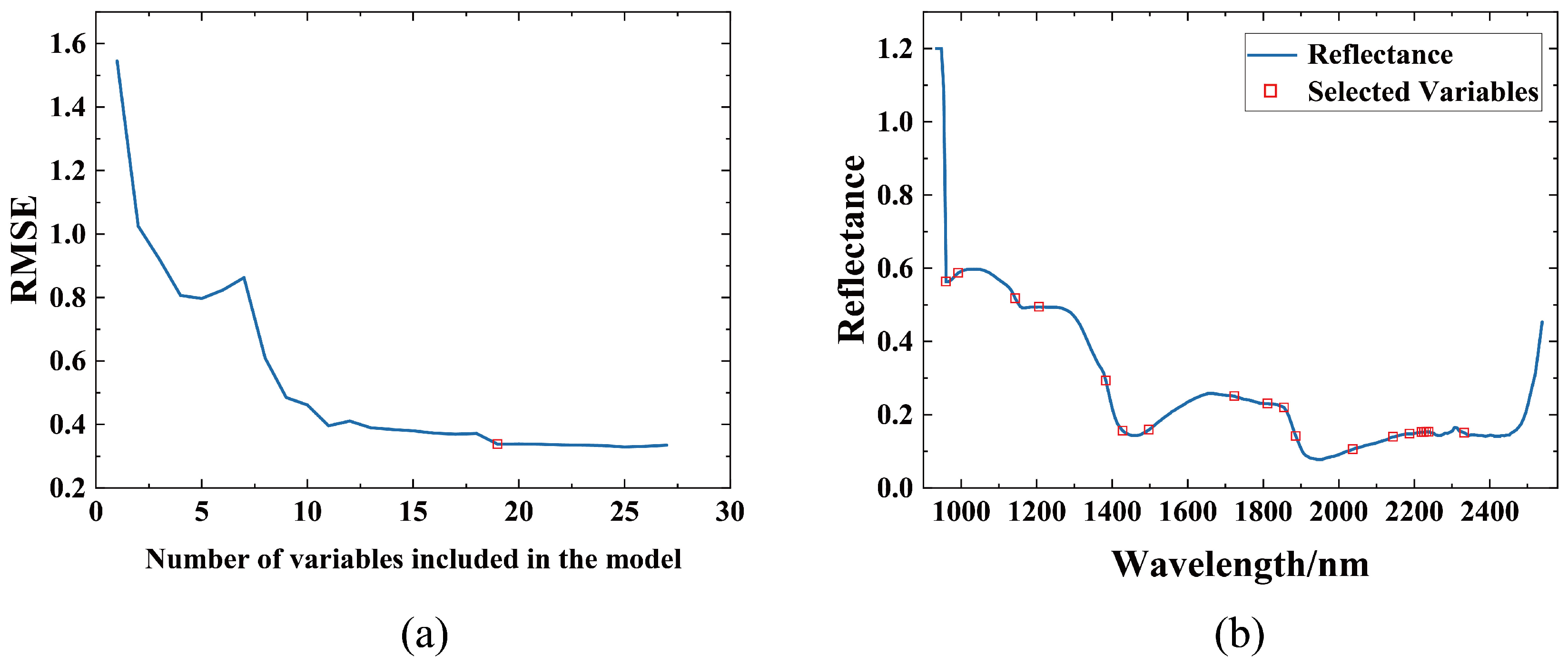
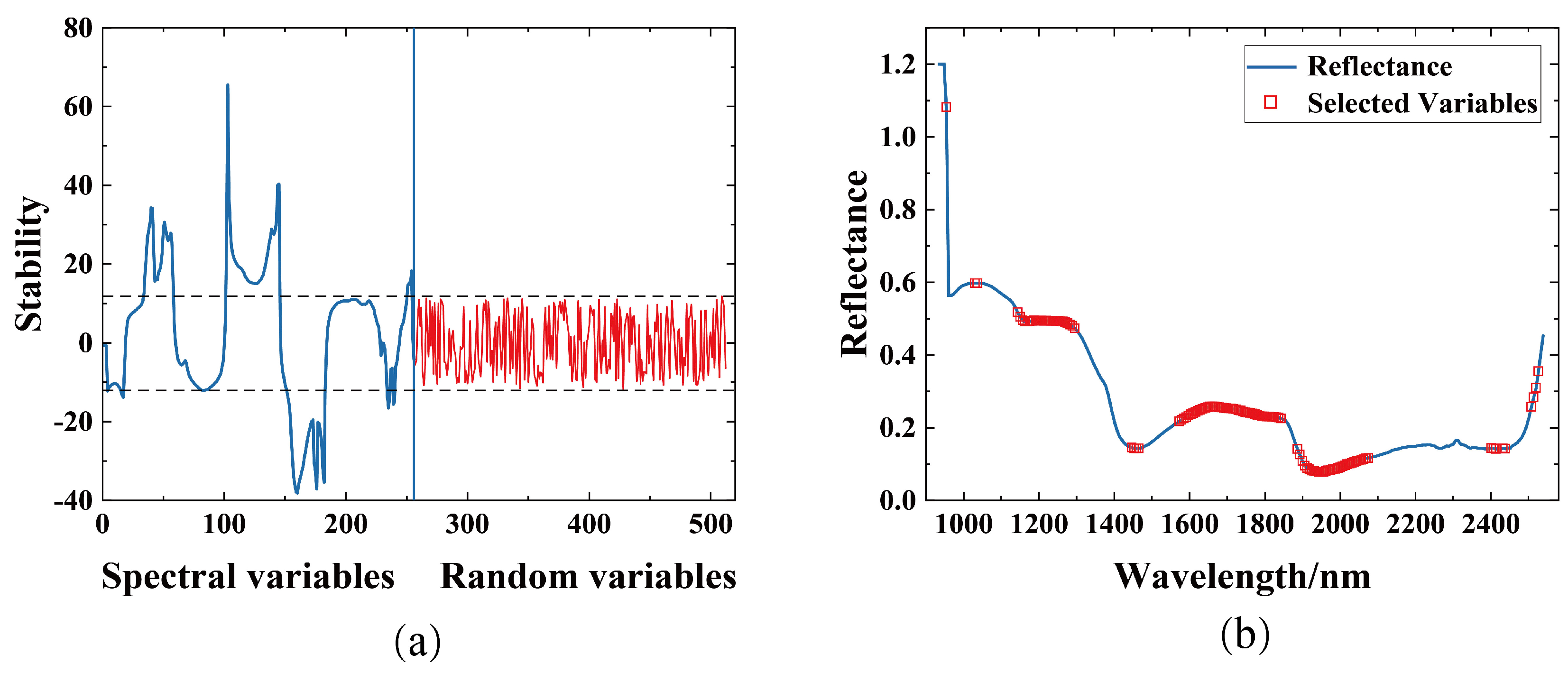
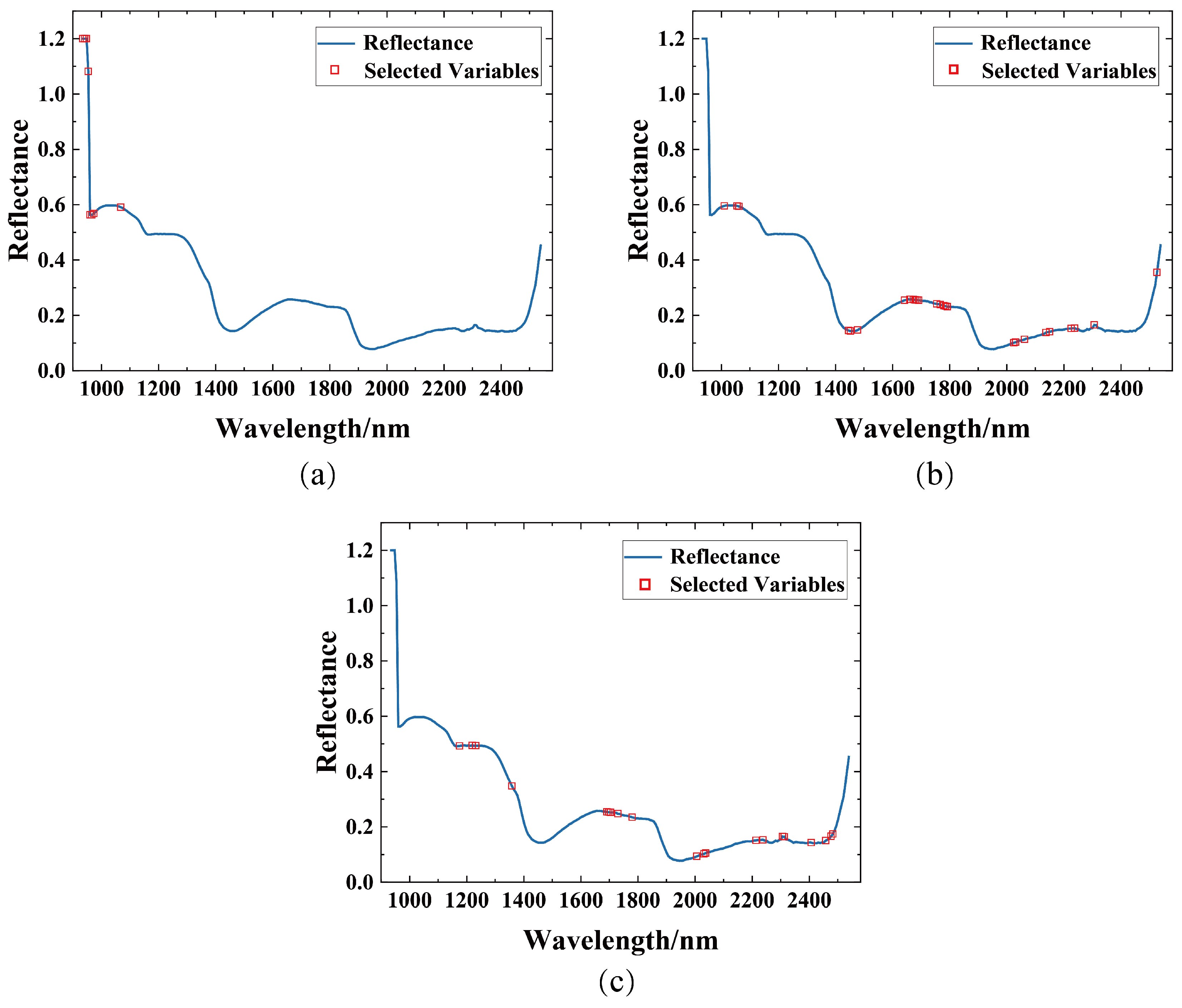
3.3. Spectral Feature Selection

There were a total of 256 bands contained in the raw spectra, and too many bands and useless bands will affect the speed and accuracy of modelling; therefore, in order to reduce the redundancy of the model and improve its prediction ability, we used six methods to extract the feature bands from the raw spectra. The six methods are CARS, SPA, DWT, VCPA-IRIV, UVE, and BOSS.

When the CARS algorithm was used to screen spectral variables, the characteristic wavelengths were extracted using a 10-fold cross-validation method. The number of Monte Carlo sampling runs was set to 100. As shown in Figure 5a, the number of CARS-preferred characteristic wavelength variables decreased with an increase in the number of sampling runs. Figure 5b indicates that the root-mean-square error of the cross-validation (RMSECV) decreased slowly and then increased gradually with an increase in the number of sampling runs, which suggests that CARS over-screening occurs after the 41st sampling time to the extent that sensitive wavelength variables containing valid information are excluded, resulting in a decrease in the prediction accuracy of the model and a steep increase in the RMSECV. Figure 5c indicates that the RMSECV value was the smallest at the 41st instance of sampling, when 38 characteristic wavelength variables are preferred to account for 14.84% of the whole band; the specific band distribution is shown in Figure 5d.

When the SPA was used to screen for characteristic wavelengths sensitive to the pH of maize silage, it can be seen from Figure 6a that with an increase in the number of variables, the root-mean-square error (RMSE) as a whole showed a trend of decreasing rapidly and then decreasing slowly. The change in the RMSE was no longer significant when the number of variables was 19, at which time the RMSE was 0.3378. Since too many variables would increase the computational cost and complexity of the model, 19 variables were selected as the final number of characteristic variables, accounting for 7.42% of the whole bands. Figure 6b shows the specific distribution of these 19 bands.

In Figure 7a showing the use of the UVE algorithm for extracting feature wavelengths, the distribution of the stabilization coefficients of the 256 spectral variables under full-spectrum conditions is shown on the left side of the vertical line. The distribution of the coefficients of the 256 noise variables is shown on the right side of the vertical line. The two horizontal lines determined by the stabilization values of the variables indicate screenings for the thresholds of the spectral bands. All of the spectral bands between the horizontal lines were treated as unknown variables and deleted, and the spectral bands outside the horizontal lines were retained as helpful information. In total, 116 feature bands accounted for 45.31% of the spectral bands after screening, and the specific band distribution is shown in Figure 7b.

The DWT algorithm’s role in extracting the feature bands was based on the Matlab platform, using the Wavelet toolbox to perform a discrete wavelet transform the spectral signals. The daubechies 4 (db4) wavelet was used to decompose the original spectral signals, and finally, eight variables were selected as the final number of feature variables, accounting for 3.1% of the full band; Figure 8a shows the eight specific distributions of the bands. The VCPA-IRIV algorithm extracted the feature wavelengths by setting the sampling time of the binary matrix sampling (BMS) method to 1000, i.e., the exponential decay function (EDF) was set to 50, and the number of iterations was set to 50. Finally, 26 feature variables were screened which accounted for 10.16% of the whole band with an RMSECV value of 0.4135; the distribution of the feature wavelengths is shown in Figure 8b. The BOSS algorithm filtered the effective wavelengths that characterize the maize silage pH value. The process of feature removal followed the law of soft contraction. Less important wavelengths were not directly eliminated but assigned smaller weight values, and iterative runs were performed until the number of variables was reduced to one. The number of WBS operations was set to 1000 before the BOSS algorithm was used. The BOSS algorithm used in this study selected 20 feature variables which accounted for 7.81% of the full wavelengths with an RMSECV value of 0.4148; the distribution of the feature wavelengths is shown in Figure 8c.

Table 4. Effective variables extracted using different methods.

Extraction Method	Number of Variables	Selected Wavelength (nm)
CARS	38	1169, 1213, 1225, 1339, 1446, 1515–1534, 1679–1698, 1710–1723, 1786–1811, 1987, 2025, 2037, 2050, 2062, 2069, 2213, 2238, 2244, 2307, 2313, 2345, 2351, 2357, 2457
SPA	19	960, 992, 1143, 1207, 1383, 1427, 1496, 1723, 1811, 1855, 1887, 2037, 2144, 2188, 2219, 2225, 2232, 2238, 2332
UVE	116	954, 1030, 1036, 1143–1295, 1446, 1452, 1459, 1465, 1572–1836, 1887–2069, 2401, 2407, 2413, 2432, 2439, 2507, 2514, 2520, 2526
DWT	8	935–973, 1068
VCPA-IRIV	26	1011, 1055, 1061, 1446, 1452, 1478, 1641, 1660.66, 1673–1692
BOSS	20	1175, 1219, 1232, 1358, 1692–1704, 1729, 1780, 2006, 2031, 2037, 2213, 2238, 2307, 2313, 2407, 2457, 2476, 2482

shows the specific characteristic wavelengths selected by the six methods: CARS, the SPA, UVE, the DWT, the VCPA-IRIV algorithm, and BOSS. These wavelengths account for 14.84%, 7.42%, 45.31%, 3.1%, 10.16%, and 7.81% of the whole band, respectively. This selection significantly reduced the model’s complexity. These characteristic wavelengths contain critical information pertinent to the pH of maize silage. Therefore, 38, 19, 116, 8, 26, and 20 wavelengths extracted from the six methods were utilized as inputs for the calibration model.

3.4. Model Results and Analysis

After extracting characteristic wavelengths using the six methods, a quantitative model for predicting the pH value of maize silage was established by combining them with the PLS, SVR, and ELM algorithms. The results are shown in

Table 5. Results of six feature wavelength extraction methods using PLS, SVR, and ELM models.

	Extraction Method	Calibration Set		Prediction Set
		${\mathit{R}}_{\mathit{C}}^2$	RMSEC	${\mathit{R}}_{\mathit{P}}^2$	RMSEP	RPD
PLS	CARS	0.8905	0.5046	0.8889	0.5118	3.0258
	SPA	0.7757	0.7237	0.7700	0.7321	2.0944
	UVE	0.7798	0.7130	0.7790	0.7255	2.1363
	DWT	0.5522	1.0252	0.5352	1.0316	1.4679
	VCPA-IRIV	0.8703	0.5447	0.8604	0.5897	2.6793
	BOSS	0.9118	0.4552	0.8937	0.4753	3.0933
	RAW	0.9384	0.4214	0.6707	0.6821	1.9959
SVR	CARS	0.9666	0.2967	0.8335	0.4583	2.4514
	SPA	0.9732	0.2653	0.7173	0.5973	2.3765
	UVE	0.9579	0.3329	0.7570	0.5537	2.3256
	DWT	0.8082	0.7108	0.0387	1.1451	1.1174
	VCPA-IRIV	0.9633	0.3107	0.7744	0.5335	2.1260
	BOSS	0.9621	0.3157	0.8413	0.4475	2.5495
	RAW	0.9692	0.2846	0.7162	0.5985	2.2118
ELM	CARS	0.9220	0.4210	0.9092	0.4807	3.3238
	SPA	0.8996	0.4924	0.8699	0.5136	2.7955
	UVE	0.8913	0.5089	0.8220	0.6206	2.3928
	DWT	0.6639	0.8789	0.6574	0.9183	1.7304
	VCPA-IRIV	0.9126	0.4286	0.9074	0.5398	3.3709
	BOSS	0.9289	0.4027	0.9241	0.4372	3.6565
	RAW	0.7900	0.6930	0.7886	0.7270	2.2169

, from which we can see that the prediction performance of the DWT–PLS model was the worst among the PLS models, with a coefficient of determination of the prediction set $R_P^2$ of 0.5352 and an RPD of only 1.4679. The accuracy of the models built using the five feature extraction algorithms other than the DWT algorithm in combination with the PLS algorithm were significantly improved by the feature-variable PLS compared to the PLS model built using the original spectra. The BOSS–PLS model predicted the best results with $R_C^2$, $R_P^2,$ and RPD values of 0.9118, 0.8937, and 3.0933, respectively. Among the SVR models, the DWT–SVR model showed the worst model prediction performance, with a prediction set coefficient of determination $R_P^2$ of −0.03875 and an RPD of only 1.1174. The BOSS–SVR model demonstrated the best prediction, which was similar to the results of the PLS model. This similarity indicates that BOSS effectively eliminated redundancy in the spectral variables while preserving those highly correlated with the maize silage pH value. The model achieved $R_C^2$, $R_P^2,$ and RPD values of 0.9621, 0.8413, and 2.5495, respectively. The ELM had the best prediction results overall among the three models, with RPD predictions ranging from 1.7304 to 3.6565. Among them, the DWT–ELM model had the worst prediction results due to the collinear relationship between the effective variables. The BOSS–ELM model achieved the best prediction results, with $R_C^2$, $R_P^2$, and RPD values of 0.9289, 0.9241, and 3.6565, respectively. In addition, the coefficients of determination of the calibration and prediction sets of the BOSS–ELM model differed by only 0.0048, indicating that the model has good generalization ability and a certain degree of stability. Finally, among the three modelling algorithms, the model constructed using the BOSS feature extraction method outperformed all of the other methods, with the number of wavelengths accounting for only 7.81% of the whole band, which better selects the wavelengths relevant to the maize silage pH value and dramatically reduces the complexity and redundancy of the model, demonstrating the applicability of this algorithm for the quantitative prediction of the pH of maize silage.

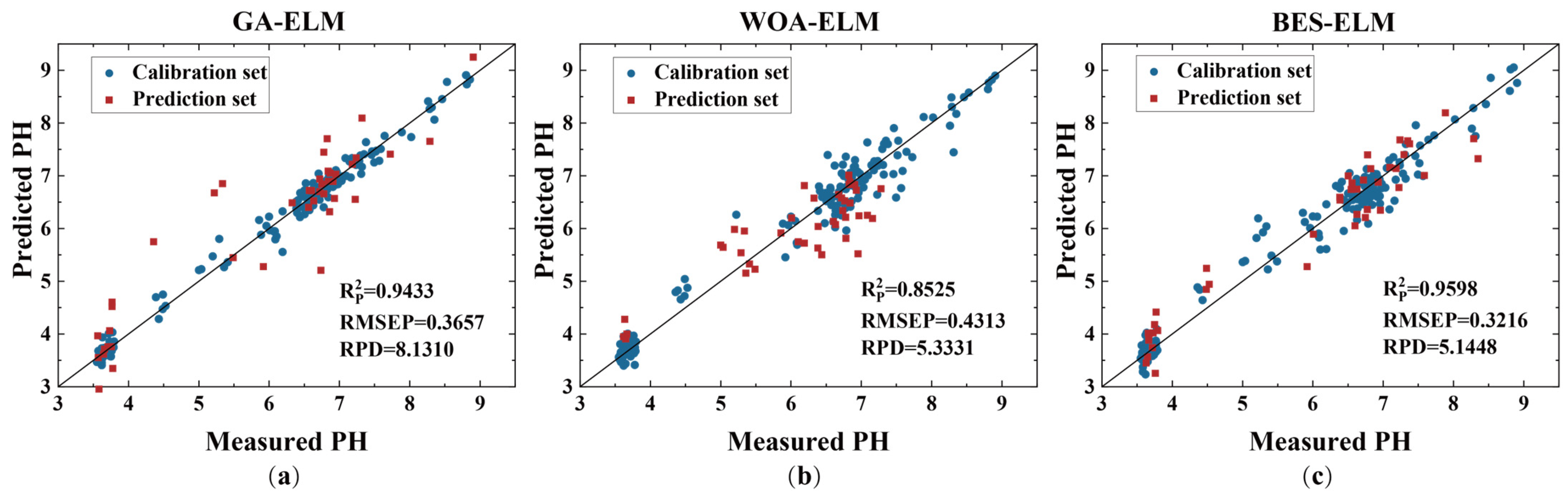
3.5. Model Optimization

For subsequent accurate predictions of pH at each pixel point in hyperspectral images, this study proposes three search optimization algorithms to optimize the BOSS–ELM model and screen the optimal model to visualize and analyze the pH of maize silage: the GA, WOA, and BES.

In the ELM model, we set the bounds of the weights W from to −1 to 1, the bounds of the bias b from to 0 to 1, and the activation function to sigmoid. In the case of the same dataset, the following optimal parameters were determined through multiple trials with 50 runs of the model in each trial: the number of GA–ELM hidden layers was set to 90, the population size was set to 20, and the number of iterations was set to 300; the number of WOA–ELM hidden layers was set to 20, the population size was set to 30, and the number of iterations was set to 100; and the number of BES–ELM hidden layers was set to 30, the population size was set to 20 and the number of iterations was set to 300. The results are shown in

Table 6. Predicted maize silage pH values based on ELM model and different optimization algorithms.

Extraction Method	Calibration Set		Prediction Set
	${\mathit{R}}_{\mathit{C}}^2$	RMSEC	${\mathit{R}}_{\mathit{P}}^2$	RMSEP	RPD
BOSS–GA–ELM	0.9848	0.1868	0.9433	0.3657	8.1310
BOSS–WOA–ELM	0.9648	0.3044	0.8525	0.4313	5.3331
BOSS–BES–ELM	0.9622	0.2923	0.9598	0.3216	5.1448

; it can be seen that the prediction accuracy of the calibration set model was improved after the three optimization algorithms were used to optimize the ELM model. However, in the prediction set model, the WOA algorithm’s prediction accuracy was reduced after the optimization, which may have been due to overfitting. When the GA and BES were used to optimize the ELM models, the prediction set prediction accuracy $R_P^2$ improved by 0.0192 and 0.0357, respectively, and the RMSEP also decreased. The results show that the BOSS–BES–ELM model achieved the best accuracy in predicting the pH of maize silage. The BES optimization algorithm determined the optimal W and B and improved the prediction accuracy of the ELM model. The prediction accuracies of the BES-optimized ELM model on the calibration set $R_C^2$ and prediction set $R_P^2$ were 0.9622 and 0.9598, respectively. A scatter plot of the results of the quantitative pH prediction model at each stage of the maize silage production process is shown in Figure 9. The solid line is the regression line, and the closer the sample points are to the regression line, the better the model will predict the pH of maize silage.

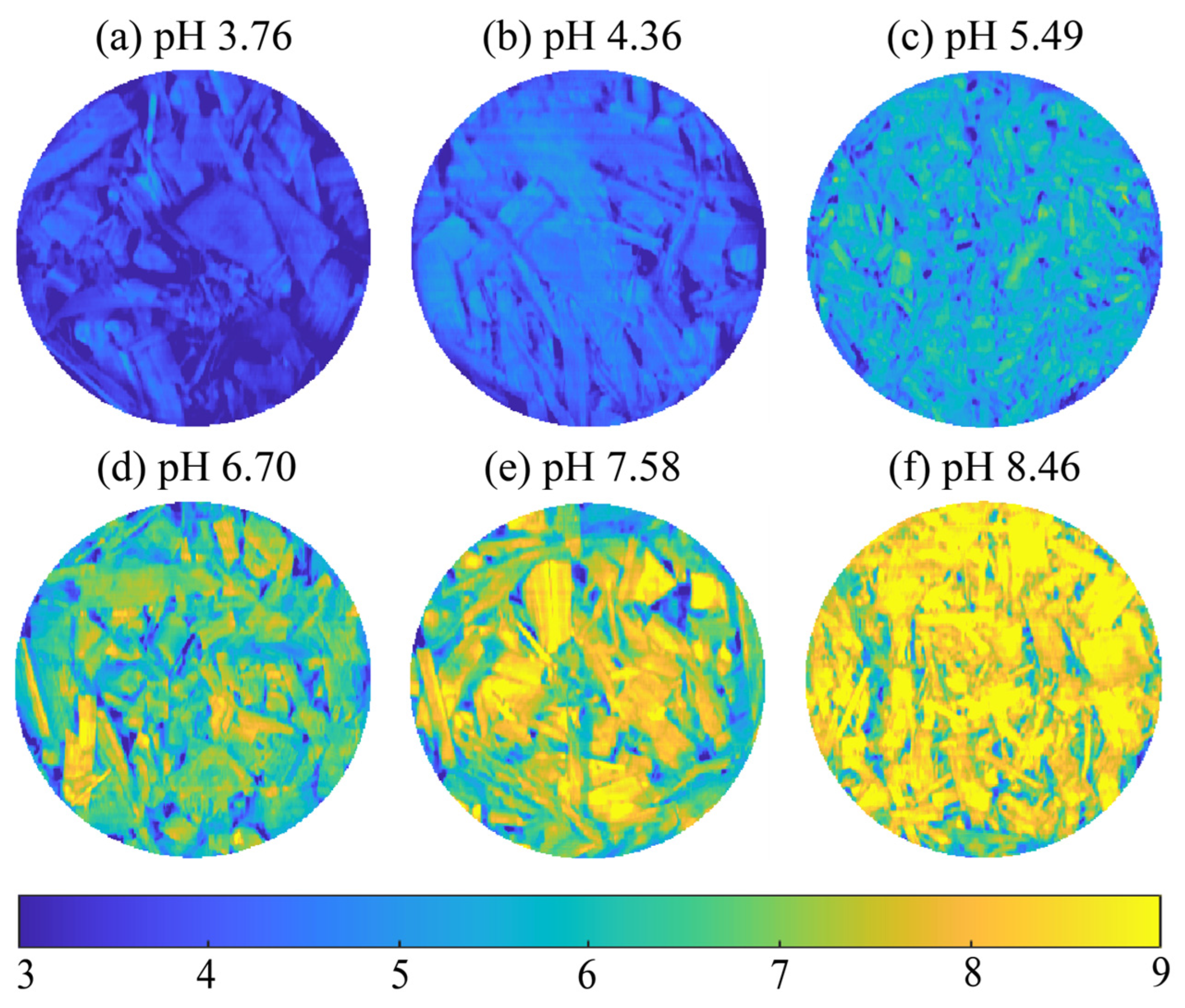
3.6. pH Value Visualization

After identifying BOSS–BES–ELM as the best quantitative prediction model, we used the model to visualize and analyze the pH of maize silage. The spectral reflectance of each pixel in the hyperspectral image of maize silage was extracted, and corresponding pH values were calculated based on the model, with an experimental pH value range of 3–9. pH value distribution maps were generated by mapping the pH value of each pixel to a gray scale range of 0–255, which was then processed into a pseudo-color image. As shown in Figure 10, areas with lower pH values are represented by darker shades of blue, while higher pH values transition to yellow. This color gradient from dark blue to yellow visually indicates an increase in pH value. Pseudo-color imaging highlights the uneven pH value distribution in the sample, allowing for clear regional differentiation. HSI offers enhanced capabilities by providing a detailed visualization of localized areas in maize silage compared to traditional near-infrared spectroscopy. This advanced visualization supports an accurate assessment of the fermentation state of silage, providing a key tool for quality analysis and control.

4. Discussion

In this study, the combination of the BOSS algorithm and the ELM model (BOSS–ELM) performed the best among all of the examined feature extraction methods ($R_P^2$ = 0.9241, RMSEP = 0.4372, and RPD = 3.6565), providing higher accuracy and stability compared to the other methods. According to recent studies such as that of Xu et al. [43], who utilized spectral imaging to predict kiwifruit SSC values, the BOSS–ELM model provided the best prediction of kiwifruit SSC, with $R_P^2$, $R_C^2$, and RPD values of 0.8894, 0.9429, and 2.88, respectively, compared to the slightly lower prediction performance of the BOSS–PLSR model with $R_P^2$, $R_C^2$, and RPD values of 0.8717, 0.8747, and 2.89, respectively. This suggests that the efficiency of the BOSS algorithm in the feature selection phase may be a key factor in improving the predictive performance of the model. In addition, our model showed a significant improvement in performance after optimization using the BES algorithm ($R_P^2$ was improved to 0.9598, the RMSEP was reduced to 0.3216, and the RPD was improved to 5.1448), and this improvement shows the potential of search optimization algorithms in nonlinear model tuning. Similarly, Yu et al. [38] observed improved performance by the ELM model after its optimization by the BES algorithm in their study estimating the rice nitrogen nutrient index. These comparisons demonstrate the broad applicability and potential practical applications of our approach in the prediction of agricultural product quality.

pH is an important indicator for assessing the quality of maize silage during secondary fermentation [44]. Although Sørensen, Liu, and Cozzolino et al. [9,10,11] used near-infrared spectroscopy to determine the pH of maize silage, the limitation of this technique is that only partial information about the samples can be obtained, and it is not possible to generate a comprehensive pH value profile. In their study, the accuracy of pH value detection was affected by factors such as uneven sampling locations, varying compaction, and slow sampling speed, which resulted in inhomogeneous results [45]. In contrast, the HSI method we used not only covers a wider range of samples but also generates detailed pH value distribution maps. This advantage significantly improves the accuracy and reliability of the assay, making it possible to quickly and conveniently monitor pH during the secondary fermentation of maize silage in the field. Our method was experimentally validated to outperform the near-infrared spectroscopy technique used by Sørensen, Liu, and Cozzolino et al. in terms of detection accuracy, in which our model achieved a higher coefficient of determination ($R_P^2$ = 0.9598 compared to the highest $R_P^2$ value achieved by Liu et al., $R_P^2=$ 0.79), demonstrating HSI’s ability to provide a more accurate and comprehensive method of monitoring pH, with significant advantages.

For testing maize silage quality, the use of non-destructive technology instead of manual testing is a future development trend. During the secondary fermentation of maize silage, in addition to pH, lactic acid, acetic acid, propionic acid, and butyric acid greatly influence the quality of the silage, and the corresponding spectral characterization information of each index is different [46]. In addition, acetic acid, propionic acid, butyric acid, etc., are volatile organic acids that change significantly during fermentation. Therefore, detecting volatile gases, accelerating research on intelligent and comprehensive testing methods for maize silage quality, developing testing equipment that can collect different information at the same time, extracting effective information corresponding to different vital components, and establishing a comprehensive analysis and prediction model to predict multiple key component indexes at the same time are important future research directions.

5. Conclusions

In this study, we successfully determined pH during the secondary fermentation of maize silage based on a combination of HSI and chemometrics. By comparing the effects of four spectral preprocessing algorithms on the modelling results, we can see that the MSC preprocessing algorithm effectively eliminated the scattering phenomenon in the samples and improved the modelling accuracy. In order to simplify the model, the BOSS feature extraction algorithm reduced the number of wavelengths from 256 to 20, and the ELM model built using the extracted feature wavelengths demonstrated a good generalization ability, with $R_P^2$, RMSEP, and RPD values of 0.9241, 0.4372, and 3.6565, respectively. Then, the $R_P^2$, RMSEP, and RPD values of the BOSS–ELM model optimized by the BES search optimization algorithm were improved to 0.9598, 0.3216, and 5.1448, respectively. Finally, the distribution of the content of maize silage with different pH value was generated. It was shown that the BOSS–BES–ELM model can effectively predict pH during the secondary fermentation of maize silage, which provides a basis for the rapid and portable detection of the fermentation quality of maize silage at its production site with considerable potential.

References

1. Ferraretto, L.F.; Shaver, R.D.; Luck, B.D. Silage Review: Recent Advances and Future Technologies for Whole-Plant and Fractionated Corn Silage Harvesting. J. Dairy Sci. 2018, 101, 3937–3951. [Google Scholar] [CrossRef] [PubMed]
2. Serva, L.; Andrighetto, I.; Segato, S.; Marchesini, G.; Chinello, M.; Magrin, L. Assessment of Maize Silage Quality under Different Pre-Ensiling Conditions. Data 2023, 8, 117. [Google Scholar] [CrossRef]
3. Liu, Y.; Wang, G.; Wu, H.; Meng, Q.; Khan, M.Z.; Zhou, Z. Effect of Hybrid Type on Fermentation and Nutritional Parameters of Whole Plant Corn Silage. Animals 2021, 11, 1587. [Google Scholar] [CrossRef] [PubMed]
4. Wilkinson, J.M.; Davies, D.R. The Aerobic Stability of Silage: Key Findings and Recent Developments. Grass Forage Sci. 2013, 68, 1–19. [Google Scholar] [CrossRef]
5. Borreani, G.; Tabacco, E.; Schmidt, R.J.; Holmes, B.J.; Muck, R.E. Silage Review: Factors Affecting Dry Matter and Quality Losses in Silages. J. Dairy Sci. 2018, 101, 3952–3979. [Google Scholar] [CrossRef] [PubMed]
6. Tharangani, R.M.H.; Yakun, C.; Zhao, L.S.; Ma, L.; Liu, H.L.; Su, S.L.; Shan, L.; Yang, Z.N.; Kononoff, P.J.; Weiss, W.P.; et al. Corn Silage Quality Index: An Index Combining Milk Yield, Silage Nutritional and Fermentation Parameters. Anim. Feed Sci. Technol. 2021, 273, 114817. [Google Scholar] [CrossRef]
7. Kung, L.; Shaver, R.D.; Grant, R.J.; Schmidt, R.J. Silage Review: Interpretation of Chemical, Microbial, and Organoleptic Components of Silages. J. Dairy Sci. 2018, 101, 4020–4033. [Google Scholar] [CrossRef] [PubMed]
8. Kumaravelu, C.; Gopal, A. A Review on the Applications of Near-Infrared Spectrometer and Chemometrics for the Agro-Food Processing Industries. In Proceedings of the 2015 IEEE Technological Innovation in ICT for Agriculture and Rural Development (TIAR), Chennai, India, 10–12 July 2015; IEEE: Piscataway, NJ, USA, 2015; pp. 8–12. [Google Scholar]
9. Sørensen, L.K. Prediction of Fermentation Parameters in Grass and Corn Silage by Near Infrared Spectroscopy. J. Dairy Sci. 2004, 87, 3826–3835. [Google Scholar] [CrossRef]
10. Liu, X.; Han, L. Prediction of Chemical Parameters in Maize Silage by near Infrared Reflectance Spectroscopy. J. Near Infrared Spectrosc. 2006, 14, 333–339. [Google Scholar] [CrossRef]
11. Cozzolino, D.; Fassio, A.; Fernández, E.; Restaino, E.; La Manna, A. Measurement of Chemical Composition in Wet Whole Maize Silage by Visible and near Infrared Reflectance Spectroscopy. Anim. Feed Sci. Technol. 2006, 129, 329–336. [Google Scholar] [CrossRef]
12. Zhang, M.; Zhao, C.; Shao, Q.; Yang, Z.; Zhang, X.; Xu, X.; Hassan, M. Determination of Water Content in Corn Stover Silage Using Near-Infrared Spectroscopy. Int. J. Agric. Biol. Eng. 2019, 12, 143–148. [Google Scholar] [CrossRef]
13. Lu, Y.; Huang, Y.; Lu, R. Innovative Hyperspectral Imaging-Based Techniques for Quality Evaluation of Fruits and Vegetables: A Review. Appl. Sci. 2017, 7, 189. [Google Scholar] [CrossRef]
14. Özdoğan, G.; Lin, X.; Sun, D.-W. Rapid and Noninvasive Sensory Analyses of Food Products by Hyperspectral Imaging: Recent Application Developments. Trends Food Sci. Technol. 2021, 111, 151–165. [Google Scholar] [CrossRef]
15. Hu, Y.; Huang, P.; Wang, Y.; Sun, J.; Wu, Y.; Kang, Z. Determination of Tibetan Tea Quality by Hyperspectral Imaging Technology and Multivariate Analysis. J. Food Compos. Anal. 2023, 117, 105136. [Google Scholar] [CrossRef]
16. Wang, Z.; Fan, S.; Wu, J.; Zhang, C.; Xu, F.; Yang, X.; Li, J. Application of Long-Wave near Infrared Hyperspectral Imaging for Determination of Moisture Content of Single Maize Seed. Spectrochim. Acta Part A Mol. Biomol. Spectrosc. 2021, 254, 119666. [Google Scholar] [CrossRef] [PubMed]
17. Yu, S.; Fan, J.; Lu, X.; Wen, W.; Shao, S.; Liang, D.; Yang, X.; Guo, X.; Zhao, C. Deep Learning Models Based on Hyperspectral Data and Time-Series Phenotypes for Predicting Quality Attributes in Lettuces under Water Stress. Comput. Electron. Agric. 2023, 211, 108034. [Google Scholar] [CrossRef]
18. Yao, X.; Cai, F.; Zhu, P.; Fang, H.; Li, J.; He, S. Non-Invasive and Rapid pH Monitoring for Meat Quality Assessment Using a Low-Cost Portable Hyperspectral Scanner. Meat Sci. 2019, 152, 73–80. [Google Scholar] [CrossRef] [PubMed]
19. Ma, T.; Xia, Y.; Inagaki, T.; Tsuchikawa, S. Non-Destructive and Fast Method of Mapping the Distribution of the Soluble Solids Content and pH in Kiwifruit Using Object Rotation near-Infrared Hyperspectral Imaging Approach. Postharvest Biol. Technol. 2021, 174, 111440. [Google Scholar] [CrossRef]
20. Wei, X.; Huang, L.; Li, S.; Gao, S.; Jie, D.; Guo, Z.; Zheng, B. Fast Determination of Amylose Content in Lotus Seeds Based on Hyperspectral Imaging. Agronomy 2023, 13, 2104. [Google Scholar] [CrossRef]
21. Yang, C.; Zhao, Y.; An, T.; Liu, Z.; Jiang, Y.; Li, Y.; Dong, C. Quantitative Prediction and Visualization of Key Physical and Chemical Components in Black Tea Fermentation Using Hyperspectral Imaging. LWT 2021, 141, 110975. [Google Scholar] [CrossRef]
22. GB/T 5009.237-2016; National Standard for Food Safety Determination of pH Value of Food. National Health and Family Planning Commission of the People’s Republic of China: Beijing, China, 2016.
23. DB15/T 1458-2018; Determination of pH Value, Organic Acid and Ammonium Nitrogen in Silage. Inner Mongolia Autonomous Region Bureau of Quality and Technical Supervision: Hohhot of Inner Mongolia Autonomous Region, China, 2018.
24. He, H.-J.; Wang, Y.; Wang, Y.; Liu, H.; Zhang, M.; Ou, X. Simultaneous Quantifying and Visualizing Moisture, Ash and Protein Distribution in Sweet Potato [Ipomoea batatas (L.) Lam] by NIR Hyperspectral Imaging. Food Chem. X 2023, 18, 100631. [Google Scholar] [CrossRef] [PubMed]
25. Kamruzzaman, M.; Makino, Y.; Oshita, S. Parsimonious Model Development for Real-Time Monitoring of Moisture in Red Meat Using Hyperspectral Imaging. Food Chem. 2016, 196, 1084–1091. [Google Scholar] [CrossRef]
26. Li, Y.; Ma, B.; Li, C.; Yu, G. Accurate Prediction of Soluble Solid Content in Dried Hami Jujube Using SWIR Hyperspectral Imaging with Comparative Analysis of Models. Comput. Electron. Agric. 2022, 193, 106655. [Google Scholar] [CrossRef]
27. Kucha, C.T.; Liu, L.; Ngadi, M.; Claude, G. Hyperspectral Imaging and Chemometrics as a Non-Invasive Tool to Discriminate and Analyze Iodine Value of Pork Fat. Food Control 2021, 127, 108145. [Google Scholar] [CrossRef]
28. Chu, Y.W.; Tang, S.S.; Ma, S.X.; Ma, Y.Y.; Hao, Z.Q.; Guo, Y.M.; Guo, L.B.; Lu, Y.F.; Zeng, X.Y. Accuracy and Stability Improvement for Meat Species Identification Using Multiplicative Scatter Correction and Laser-Induced Breakdown Spectroscopy. Opt. Express 2018, 26, 10119. [Google Scholar] [CrossRef] [PubMed]
29. Zhang, D.; Xu, Y.; Huang, W.; Tian, X.; Xia, Y.; Xu, L.; Fan, S. Nondestructive Measurement of Soluble Solids Content in Apple Using near Infrared Hyperspectral Imaging Coupled with Wavelength Selection Algorithm. Infrared Phys. Technol. 2019, 98, 297–304. [Google Scholar] [CrossRef]
30. Wang, Y.-J.; Jin, G.; Li, L.-Q.; Liu, Y.; Kianpoor Kalkhajeh, Y.; Ning, J.-M.; Zhang, Z.-Z. NIR Hyperspectral Imaging Coupled with Chemometrics for Nondestructive Assessment of Phosphorus and Potassium Contents in Tea Leaves. Infrared Phys. Technol. 2020, 108, 103365. [Google Scholar] [CrossRef]
31. Bruce, L.M.; Koger, C.H.; Jiang, L. Dimensionality Reduction of Hyperspectral Data Using Discrete Wavelet Transform Feature Extraction. IEEE Trans. Geosci. Remote Sens. 2002, 40, 2331–2338. [Google Scholar] [CrossRef]
32. Dai, F.; Shi, J.; Yang, C.; Li, Y.; Zhao, Y.; Liu, Z.; An, T.; Li, X.; Yan, P.; Dong, C. Detection of Anthocyanin Content in Fresh Zijuan Tea Leaves Based on Hyperspectral Imaging. Food Control 2023, 152, 109839. [Google Scholar] [CrossRef]
33. Centner, V.; Massart, D.-L.; De Noord, O.E.; De Jong, S.; Vandeginste, B.M.; Sterna, C. Elimination of Uninformative Variables for Multivariate Calibration. Anal. Chem. 1996, 68, 3851–3858. [Google Scholar] [CrossRef]
34. Deng, B.-C.; Yun, Y.-H.; Cao, D.-S.; Yin, Y.-L.; Wang, W.-T.; Lu, H.-M.; Luo, Q.-Y.; Liang, Y.-Z. A Bootstrapping Soft Shrinkage Approach for Variable Selection in Chemical Modeling. Anal. Chim. Acta 2016, 908, 63–74. [Google Scholar] [CrossRef] [PubMed]
35. Li, F.; Wang, L.; Liu, J.; Wang, Y.; Chang, Q. Evaluation of Leaf N Concentration in Winter Wheat Based on Discrete Wavelet Transform Analysis. Remote Sens. 2019, 11, 1331. [Google Scholar] [CrossRef]
36. Yao, K.; Sun, J.; Chen, C.; Xu, M.; Cao, Y.; Zhou, X.; Tian, Y.; Cheng, J. Visualization Research of Egg Freshness Based on Hyperspectral Imaging and Binary Competitive Adaptive Reweighted Sampling. Infrared Phys. Technol. 2022, 127, 104414. [Google Scholar] [CrossRef]
37. Yu, F.; Bai, J.; Jin, Z.; Zhang, H.; Guo, Z.; Chen, C. Research on Precise Fertilization Method of Rice Tillering Stage Based on UAV Hyperspectral Remote Sensing Prescription Map. Agronomy 2022, 12, 2893. [Google Scholar] [CrossRef]
38. Yu, F.; Bai, J.; Jin, Z.; Zhang, H.; Yang, J.; Xu, T. Estimating the Rice Nitrogen Nutrition Index Based on Hyperspectral Transform Technology. Front. Plant Sci. 2023, 14, 1118098. [Google Scholar] [CrossRef] [PubMed]
39. Mirjalili, S. Genetic Algorithm. In Evolutionary Algorithms and Neural Networks; Studies in Computational Intelligence; Springer International Publishing: Cham, Switzerland, 2019; Volume 780, pp. 43–55. ISBN 978-3-319-93024-4. [Google Scholar]
40. Mirjalili, S.; Lewis, A. The Whale Optimization Algorithm. Adv. Eng. Softw. 2016, 95, 51–67. [Google Scholar] [CrossRef]
41. Alsattar, H.A.; Zaidan, A.A.; Zaidan, B.B. Novel Meta-Heuristic Bald Eagle Search Optimisation Algorithm. Artif. Intell. Rev. 2020, 53, 2237–2264. [Google Scholar] [CrossRef]
42. Yu, S.; Bu, H.; Hu, X.; Dong, W.; Zhang, L. Establishment and Accuracy Evaluation of Cotton Leaf Chlorophyll Content Prediction Model Combined with Hyperspectral Image and Feature Variable Selection. Agronomy 2023, 13, 2120. [Google Scholar] [CrossRef]
43. Xu, L.; Chen, Y.; Wang, X.; Chen, H.; Tang, Z.; Shi, X.; Chen, X.; Wang, Y.; Kang, Z.; Zou, Z.; et al. Non-Destructive Detection of Kiwifruit Soluble Solid Content Based on Hyperspectral and Fluorescence Spectral Imaging. Front. Plant Sci. 2023, 13, 1075929. [Google Scholar] [CrossRef]
44. Wang, C.; Han, H.; Sun, L.; Na, N.; Xu, H.; Chang, S.; Jiang, Y.; Xue, Y. Bacterial Succession Pattern during the Fermentation Process in Whole-Plant Corn Silage Processed in Different Geographical Areas of Northern China. Processes 2021, 9, 900. [Google Scholar] [CrossRef]
45. Wang, Y.; Liu, Y.; Chen, Y.; Cui, Q.; Li, L.; Ning, J.; Zhang, Z. Spatial Distribution of Total Polyphenols in Multi-Type of Tea Using near-Infrared Hyperspectral Imaging. LWT 2021, 148, 111737. [Google Scholar] [CrossRef]
46. Andrighetto, I.; Serva, L.; Gazziero, M.; Tenti, S.; Mirisola, M.; Garbin, E.; Contiero, B.; Grandis, D.; Marchesini, G. Proposal and Validation of New Indexes to Evaluate Maize Silage Fermentative Quality in Lab-Scale Ensiling Conditions through the Use of a Receiver Operating Characteristic Analysis. Anim. Feed Sci. Technol. 2018, 242, 31–40. [Google Scholar] [CrossRef]
Figure 1. Flowchart of the main sample collection and data analysis steps.
Agronomy 14 01204 g001
Figure 2. Schematic diagram of using the BES search algorithm to optimize the parameters of the ELM model.
Agronomy 14 01204 g002
Figure 3. Average spectra of the 192 maize silage samples.
Agronomy 14 01204 g003
Figure 4. (a) The spectra after processing using the SG method. (b) The spectra after processing using the MSC method. (c) The spectra after processing using the SNV method. (d) The spectra after processing using the first derivative.
Agronomy 14 01204 g004
Figure 5. Wavelength (variable) selection by CARS. (a) The changing trend in the number of sampled variables; (b) 10-fold RMSECV; and (c) regression coefficients of each variable with an increment in runs, where the blue line represents the position with the lowest 10-fold RMSECV. (d) Selected bands determined using the CARS algorithm.
Agronomy 14 01204 g005
Figure 6. RMSE plot (a) and variables selected for pH value (b) by SPA.
Agronomy 14 01204 g006
Figure 7. Feature wavelengths selection via UVE: (a) UVE band selection process and (b) distribution of wavelengths selected via UVE.
Agronomy 14 01204 g007
Figure 8. (a) The distribution of characteristic wavelengths screened by the DWT algorithm; (b) the distribution of characteristic wavelengths screened by the VCPA-IRIV algorithm; and (c) the distribution of characteristic wavelengths screened by the BOSS algorithm.
Agronomy 14 01204 g008
Figure 9. (a) Scatter plot of predicted versus measured pH values obtained via BOSS–GA–ELM model. (b) Scatter plot of predicted versus measured pH values obtained via BOSS–WOA–ELM model. (c) Scatter plot of predicted versus measured pH values obtained via BOSS–BES–ELM model.
Agronomy 14 01204 g009
Figure 10. Visualization of the distribution of maize silage at different pH values.
Agronomy 14 01204 g010