Inversion of Soybean Net Photosynthetic Rate Based on UAV Multi-Source Remote Sensing and Machine Learning

Abstract

Net photosynthetic rate (Pn) is a common indicator used to measure the efficiency of photosynthesis and growth conditions of plants. In this study, soybeans under different moisture gradients were selected as the research objects. Fourteen vegetation indices (VIS) and five canopy structure characteristics (CSC) (plant height (PH), volume (V), canopy cover (CC), canopy length (L), and canopy width (W)) were obtained using an unmanned aerial vehicle (UAV) equipped with three different sensors (visible, multispectral, and LiDAR) at five growth stages of soybeans. Soybean Pn was simultaneously measured manually in the field. The variability of soybean Pn under different conditions and the trend change of CSC under different moisture gradients were analysed. VIS, CSC, and their combinations were used as input features, and four machine learning algorithms (multiple linear regression, random forest, Extreme gradient-boosting tree regression, and ridge regression) were used to perform soybean Pn inversion. The results showed that, compared with the inversion model using VIS or CSC as features alone, the inversion model using the combination of VIS and CSC features showed a significant improvement in the inversion accuracy at all five stages. The highest accuracy (R² = 0.86, RMSE = 1.73 µmol m⁻² s⁻¹, RPD = 2.63) was achieved 63 days after sowing (DAS63).

1. Introduction

Photosynthesis is a complex and critical biological process in nature performed by green plants [1]. It achieves energy conversion, participates in the carbon cycle, produces oxygen, and provides the basis for the survival of other organisms in the ecosystem. This process is not only a simple chemical reaction but also a key link in the energy conversion and material cycle in the living system [2]. Green plants are able to absorb solar energy and use it to convert carbon dioxide and water into energy-rich organic matter, such as glucose, through photosynthesis. This provides energy and raw materials for the growth of plants and provides a food source for other organisms in the biosphere [3]. The net photosynthetic rate (Pn), which measures the speed of carbon dioxide absorption and oxygen release through photosynthesis per unit of time under light conditions, is a core indicator for evaluating the efficiency of plant photosynthesis. It is the value of the total photosynthetic rate minus the respiration rate and is usually used to measure the photosynthetic efficiency and growth conditions of plants. Therefore, it is particularly important to monitor plant Pn in real time to scientifically monitor plant growth conditions and effectively improve cultivation measures.

The commonly used method for measuring Pn is typically based on ground-contact measurement devices, such as the LI-COR photosynthesis meters [4,5]. However, the measurement area of these devices is limited to a single leaf, and the measurement process is time consuming and labour intensive, making it impossible to measure the entire plant of a crop and resulting in low representativeness of the data. Therefore, there is an urgent need for a method that can provide the overall Pn of the crop in a high-throughput and rapid manner. In recent years, unmanned aerial vehicle (UAV) remote sensing technology has made remarkable progress. Its advantages include wide access to information, few operational constraints, highly efficient data acquisition, and the ability to monitor crop growth dynamically. This makes it an important tool for large-area agricultural surveys and monitoring, which is crucial for the precise management of modern agriculture [6]. Considering the high efficiency, flexibility, and real-time capabilities of UAV remote sensing technology, its application in dynamic, rapid, and high-throughput monitoring of soybean Pn shows great potential and is expected to provide strong scientific support for precision management in modern agriculture.

In recent years, UAV remote sensing technology has performed particularly well in the field of crop phenotyping, providing brand-new technical means for crop growth status monitoring, physiological and ecological monitoring [7], and agricultural resource management [8]. In terms of research on crop physiological and ecological-related indicators, Zhang et al. [9] established an inverse model of leaf area index (LAI) at four stages of wheat by combining the UAV point-cloud-data-based canopy height model (CHM) with the vegetation index (VIS). The results showed that the regression model combined with CHM data increased R² by 0.020–0.268. Li et al. [10] obtained a maize canopy structure (including height and density) using UAV point cloud, LAI inversion, and canopy-structure-based multiple linear regression models. Gong et al. [11] successfully estimated the LAI of different rice varieties during the entire growth season based on the product of the VIS and canopy height using UAV remote sensing technology, with an error controlled within 24%. This method did not require parameter adjustment due to phenological changes, effectively reducing lag. Combined with machine learning, Han et al. [12] estimated maize aboveground biomass (AGB) using structural and spectral information provided by UAV remote sensing. The results showed that the random forest model had the most balanced performance, with small errors and a high explained variance ratio on both training and test sets. The importance analysis of the predictive factors showed that the three-dimensional volume index had the largest strength effect on AGB estimation among the four machine learning models. Zhang et al. [13] analysed structural indices and two chlorophyll vegetation indices using three regression algorithms. Maimaitijiang et al. [14] used satellite and UAV data fusion for crop monitoring based on machine learning. This study provided canopy spectral information and canopy structure characteristics (CSC) in soybean areas using inexpensive UAVs. Four machine learning methods were used to predict soybean LAI, AGB, and leaf nitrogen content using canopy spectral and structural information and their combinations. These studies indicated that CSC, such as plant height and canopy coverage, have good correlations with physiological and ecological indicators such as LAI, AGB, and nitrogen content, and the combination of CSC and VIS yields good results for the inversion of these physiological indicators. This provides strong support for the application of UAV remote sensing technology in crop physiological and ecological research. Since the organic matter accumulated by photosynthesis directly affects basic growth indicators of soybeans, such as plant height, volume, and canopy coverage, CSC also demonstrate great potential in estimating Pn.

In research on the inversion of crop Pn using remote sensing technology, Zhang et al. [15] established a regression model for the canopy Pn of rapeseed using the remote sensing VIS and solar-induced chlorophyll fluorescence. They also obtained a new composite index by multiplying individual indicators, improving the method for extracting the Pn of rapeseed seedlings from UAV remote sensing data. Wu et al. [16] applied inversion modelling to Pn using UAV multispectral images and found that gradient-boosting decision trees and random forest models with fused inputs could be used for estimating rice Pn. This method could also provide references for field Pn monitoring and yield prediction. Zhang et al. [17] used multispectral data obtained from UAVs to input into the LRC model to rapidly predict the diurnal variation of rice leaf photosynthetic rate. Zhang et al. [18] used six leaf phenotypic data of aspen leaves (area, length, width, perimeter, ratio, and factor) combined with four machine learning algorithms to invert leaf Pn. The results showed that the extreme gradient-boosting tree had the highest inversion accuracy, with an MAE and R² of 1.12 and 0.60, respectively. All of the above are classic cases of Pn inversion using remote sensing technology. However, few studies have been conducted on the Pn of soybean, and little attention has been paid to the effect of CSC on Pn prediction.

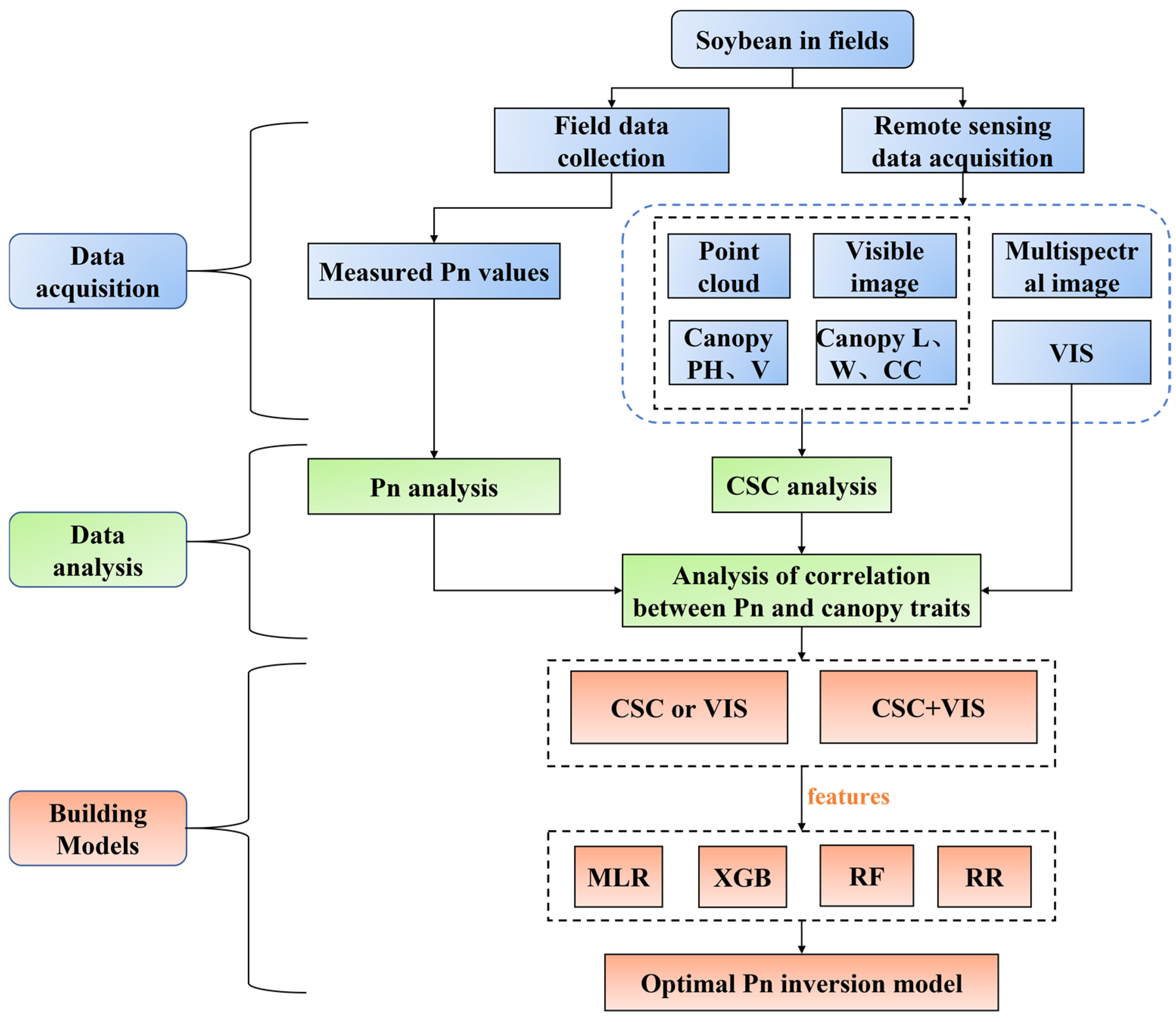
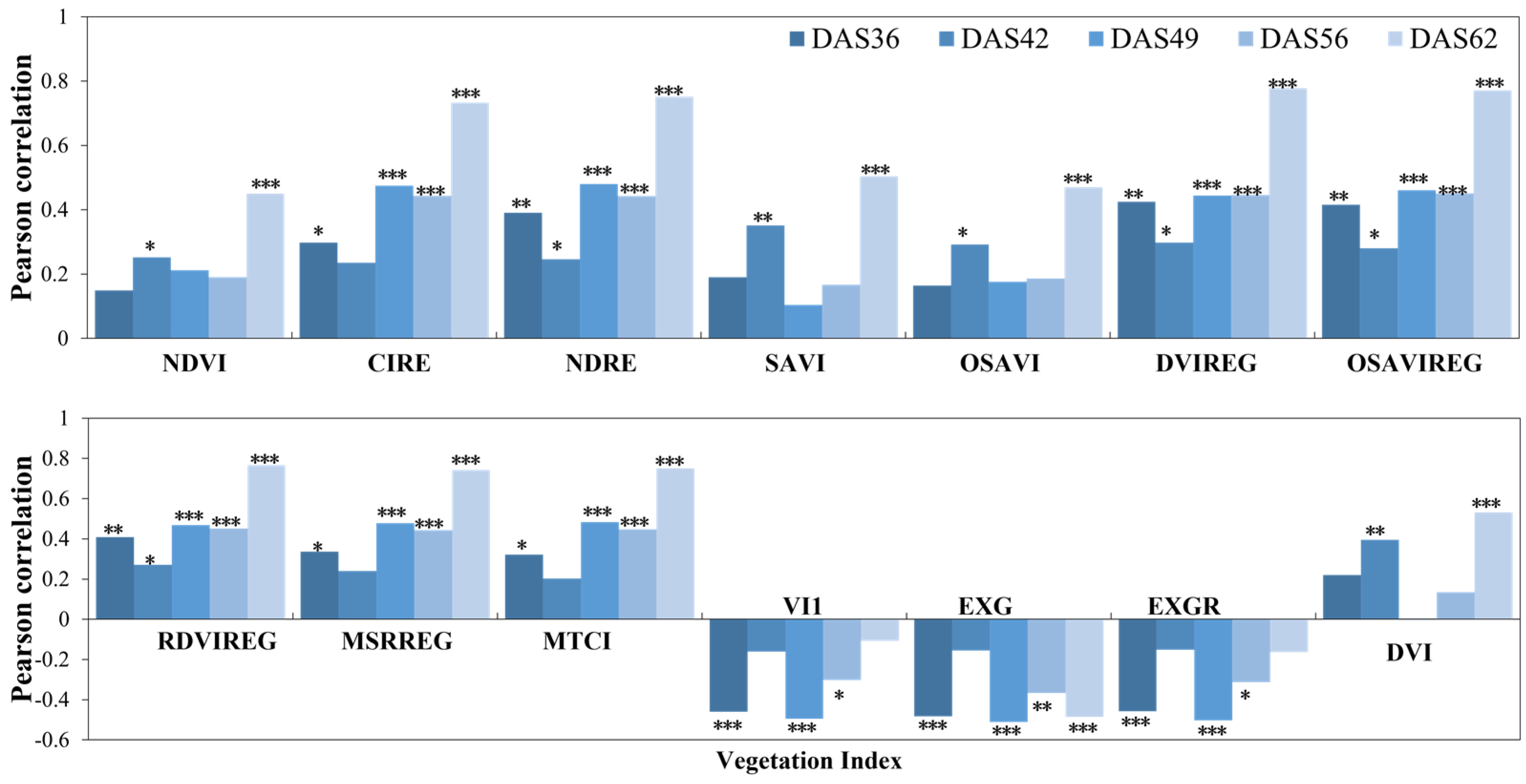
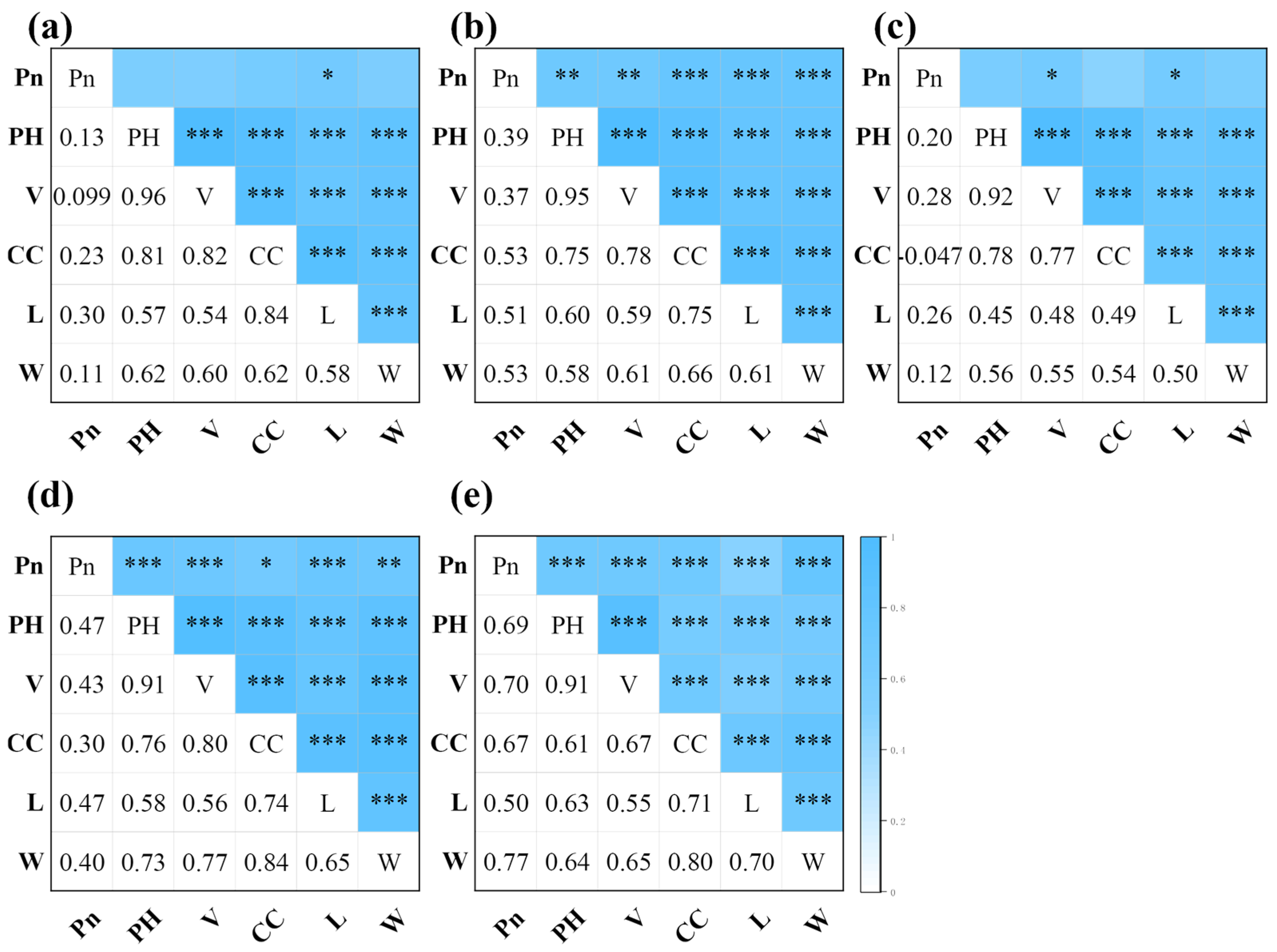
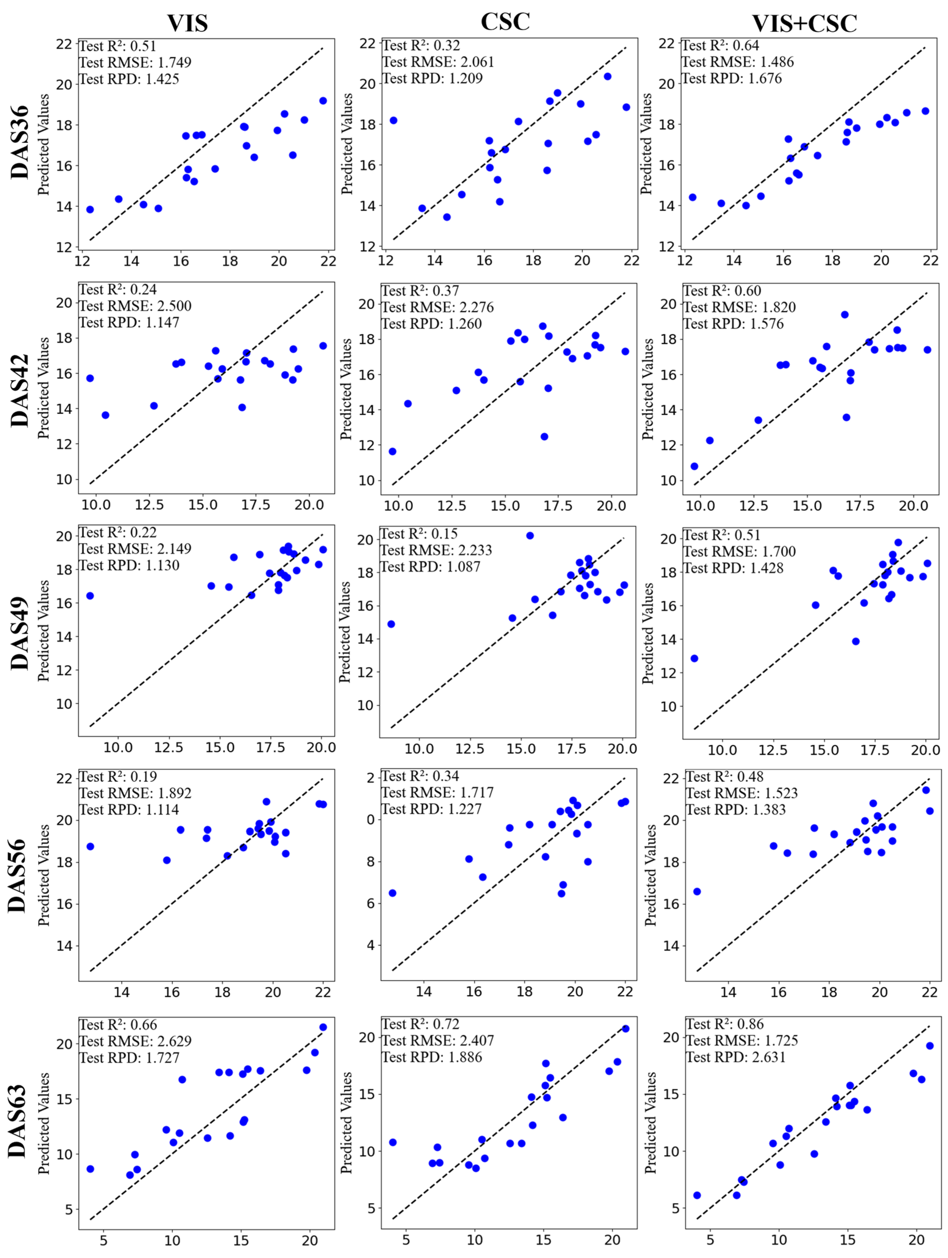
Therefore, this study focused on soybeans under different moisture gradients, obtaining visible-light and multispectral images and point cloud data of soybeans using a UAV. The differences in Pn under different conditions and the trends of CSC under different moisture gradients were analysed. The correlation between CSC, VIS, and Pn at different stages was analysed, and VIS was selected for the input into four machine learning models based on the magnitude of the correlation. The accuracy of the Pn inversion model under different input feature combinations at each stage was compared, and the inversion effect of the fusion of VIS and CSC was further analysed. The technology roadmap for this study is shown in Figure 1.

2. Materials and Methods

2.1. Study Region and Experimental Design

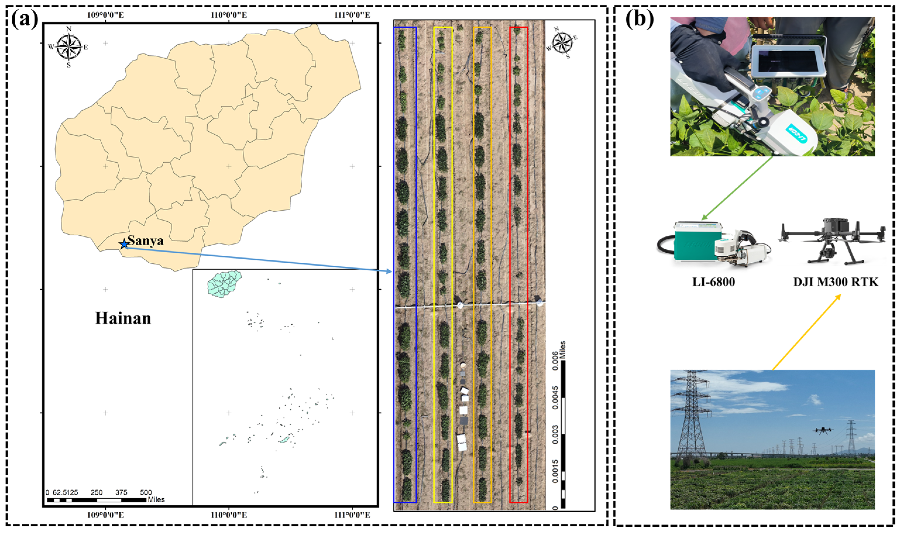
The study area was located at the experimental base of Batou, Yazhou District, Sanya City, Hainan Province, China (18°22′12″ N, 109°9′11″ E). The experimental base is located in the subtropical region and has a tropical marine monsoon climate. The average annual temperature ranges from 24.9 °C to 26 °C, the average annual sunshine duration is 2572.8 h, and the average annual precipitation is 1100–1300 mm. The area experiences distinct wet and dry seasons and has excellent air quality, making it highly suitable for soybean growth and experimentation.

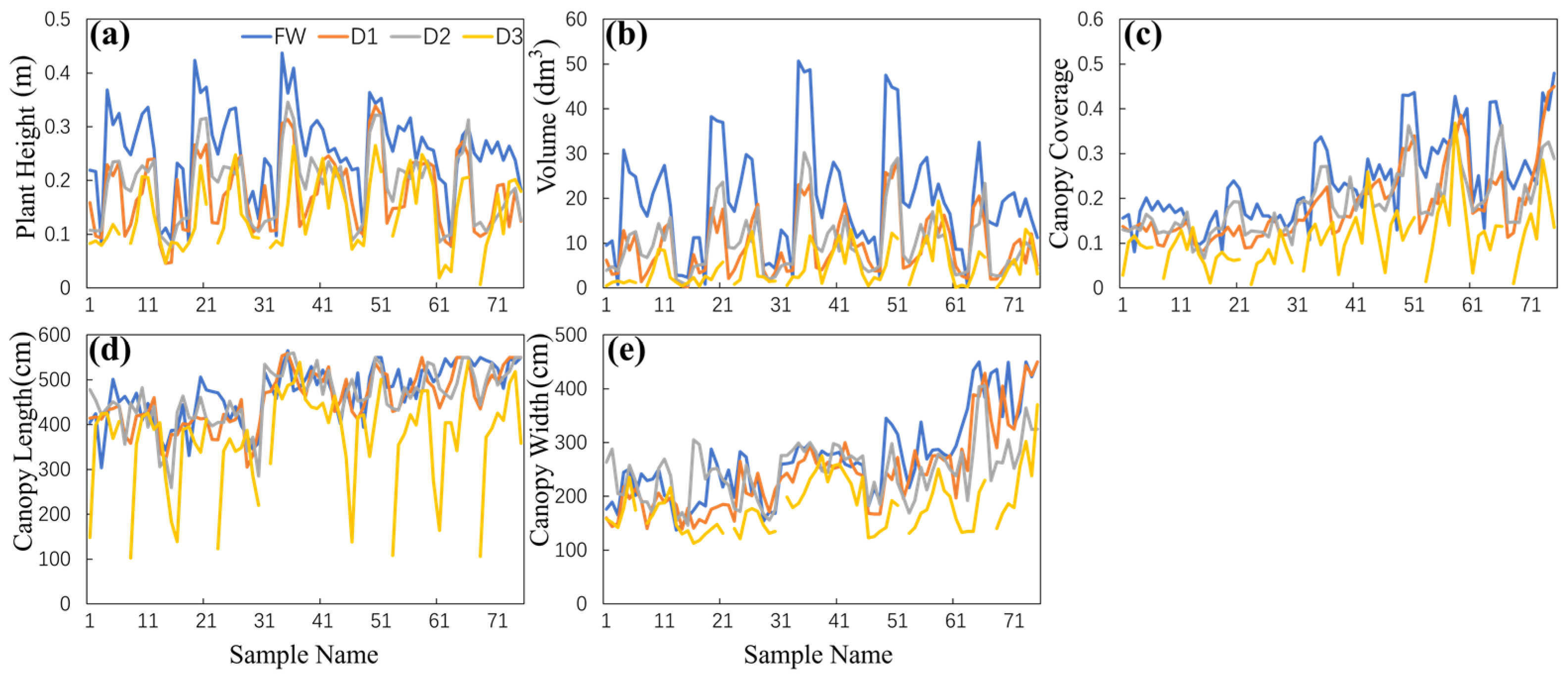
The soybean sowing for the experiment was conducted on 1 November 2023. As shown in Figure 2a, a total of four ridges were planted in the area, with each ridge containing five different soybean varieties. Each variety was planted in three plots within different ridges, for a total of 60 plots, to increase the sample size of the varieties. Double rows with a plant spacing of 0.15 m and a ridge spacing of 0.8 m were planted in each plot. Each variety was sown with 16 seedlings, that is, each plot was 1.2 m long and 0.8 m wide. Different moisture gradients, categorised into sufficiently watered (FW, relative moisture content of 80–85%), mild drought (D1, relative moisture content of 65–70%), moderate drought (D2, relative moisture content of 50–55%), and severe drought (D3, relative moisture content of 25–30%), were applied to the experimental soil. The water content of the soybeans in each row was controlled by each watering, which used a flow meter to control the amount of water flowing out of each row of pipes. Ridges were separated from each other by a ridge of land to prevent watering interfering with the moisture levels of other ridges. Due to unforeseen circumstances, one area under the D3 treatment did not emerge successfully.

2.2. Photosynthetic Rate and Unmanned Aerial Vehicle Data Collection

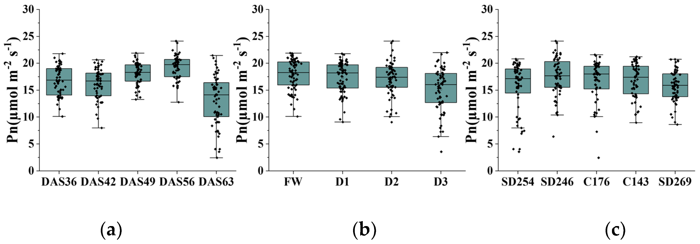
The instrument used for the measurement of Pn was the LI-6800 photosynthesis meter (LI-COR, Lincoln, NE, USA). Due to the opening and closing characteristics of plant stomata, the measurements needed to be taken before the flight operations of the UAV, which was equipped with a variety of sensors, i.e., between 8:30 and 11:30 every day. As shown in Figure 2b, the Pn of soybeans was simultaneously measured in the field. Three soybean plants were randomly selected from each plot, and measurements were taken on the third attached leaf at the top. The collected data were averaged to obtain the Pn value for each plot. Five measurements were conducted at the Yazhou experimental base during the soybean growth cycle: at the flowering, podding, beginning seed, seed-filling, and maturity stages. The measurement dates were 6 January, 12 January, 19 January, 26 January, and 3 February 2024, respectively. Since soybeans were sown on 1 November 2023, this corresponded to 36, 42, 49, 56, and 63 days after sowing (DAS). Pn samples were collected from 59 plots during each measurement for 295 samples.

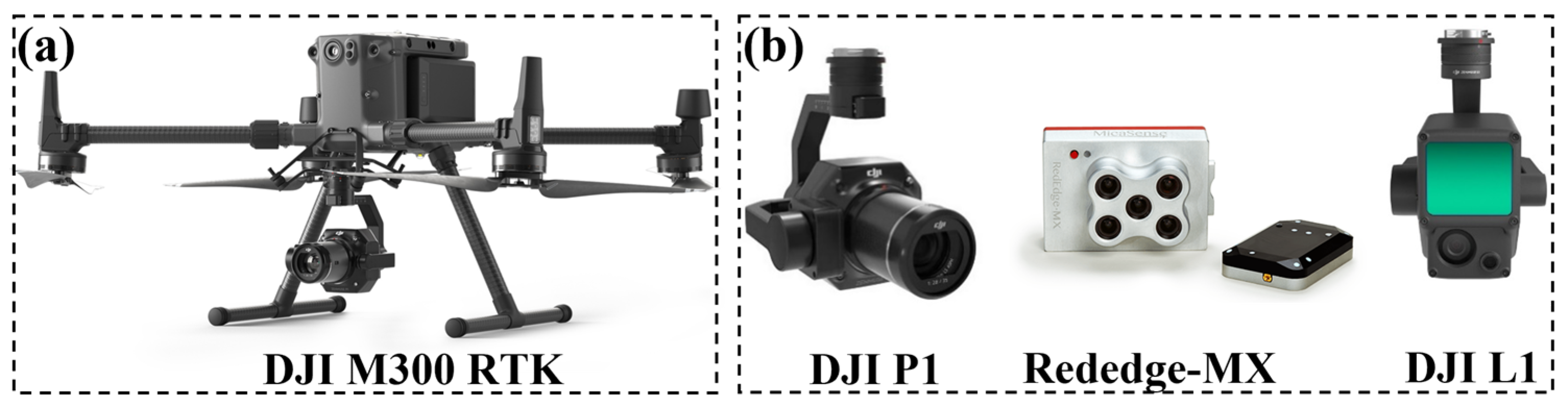
This study utilised a UAV system (Matrice 300 RTK; SZ DJI Technology Co., Ltd., Shenzhen, Guangdong, China) equipped with visible, multispectral, and LiDAR sensors to simultaneously collect three types of remote sensing images (Figure 3). The visible sensor (P1, SZ DJI Technology Co., Ltd.) had a resolution of 8192 × 5460. The multispectral sensor (Rededge-MX; MicaSense, Seattle, WA, USA) was composed of five bands with a wavelength range of 400–900 nm and a resolution of 1280 × 960. The LiDAR sensor (L1; SZ DJI Technology Co., Ltd.) had a ranging accuracy of 3 cm @ 100 m. The flight planning for the visible and multispectral sensors was identical, with a flight altitude of 30 m, 80% forward overlap, 80% side overlap, an excitation mode of isotropic velocity, an excitation interval of 1 s, and a flight speed of 2 m s⁻¹. The flight planning for the LiDAR sensor included a flight altitude of 20 m, 70% forward overlap, 20% LiDAR side overlap, 70% visible side overlap, an excitation mode of isotropic velocity, an excitation interval of 1 s, and a flight speed of 1 m s⁻¹. Two radiometric calibration panels with reflectance values of 5% and 15% were placed in the field before each flight as the digital numbers (DN) of the multispectral images needed to be converted into reflectance values during post-processing.

2.3. Canopy Structure Characteristics Data Processing

Three CSC of soybean, i.e., canopy coverage, canopy length, and canopy width, were extracted from visible images; two CSC, i.e., plant height and volume, were extracted from point cloud images; and the VIS was extracted from multispectral images. The vegetation index EXGR (Excess Green minus Excess Red) [19], on the other hand, is a vegetation index used to assess vegetation cover and growth and is calculated as shown in Equation (1) in the text. This index is particularly suitable for analysing UAV visible-light imagery to more accurately identify vegetated and non-vegetated areas. Therefore, the EXGR vegetation index combined with the OTSU thresholding method was used to binarise the visible and multispectral images and segment the soybean canopy image of the field [20]. The breakdown process diagram is shown in Figure 4. R, G, and B are the red, green, and blue bands, respectively.

EXGR = 3G − 2.4R − B

(1)

After obtaining the mask image from the visible image, the canopy coverage (CC) of the image was obtained by traversing each pixel of the image, counting the number of black and white pixels, and then calculating the proportion of white pixels to the total number of pixels. The length (L) and width (W) of the canopy were obtained by calculating the number of rows and columns occupied by white pixels.

After obtaining the mask image from the multispectral image, soybean images were extracted in the red, green, blue, near-infrared, and red-edge bands. Each soybean image was segmented into multiple regions of interest (ROIs) based on variety. The average greyscale value of each ROI image was calculated, and then the extracted greyscale values were calibrated using two reflectance calibration panels placed before the experiment to obtain reflectance values for the five bands.

Soybean plant height (PH) and volume (V) were extracted in the soybean point cloud using CloudCompare_v2.13.1 software. The height measurement tool in the CloudCompare_v2.13.1 software was used to mark the ROIs and calculate plant height, and the volume calculation tool was used to select regions or geometric shapes for volume measurement.

2.4. Calculation of Vegetation Index

VIS is a remote sensing indicator used to assess vegetation health and coverage. It is typically based on multispectral or hyperspectral image data. These indices evaluate vegetation growth status, chlorophyll content, and land cover types by calculating the relationship between different bands in the image [21]. Therefore, after obtaining the reflectance values for the five bands of the soybean canopy, the VIS was calculated, and 14 VIS indices were obtained, as shown in

Table 1. VIS calculation formulas.

VIS	Abbreviations and Calculation Formulas	References
Normalised Difference Vegetation Index	NDVI = (NIR − R)/(NIR + R)	[22]
Canopy Intercepted Radiation Estimator	CIRE = NIR − REG	[23]
Normalised Difference Red Edge	NDRE = (NIR − REG)/(NIR + REG)	[24]
Soil-Adjusted Vegetation Index	SAVI = 1.5(NIR − R)/(NIR + R + 0.5)	[25]
Optimised Soil-Adjusted Vegetation Index	OSAVI = 1.16(NIR − R)/(NIR + R + 0.16)	[26]
Difference Vegetation Index	DVIREG = NIR − G	[27]
Optimised Soil-Adjusted Vegetation Index Regression	OSAVIREG = (1 + 0.16)(NIR − G)(NIR + G + 0.16)	[28]
Regression of Ratio Vegetation Index	RDVIREG = (NIR − REG)/(NIR + REG)0.5	[29]
Modified Simple Ratio Regression	MSRREG = (NIR/REG − 1)/(NIR/REG + 1)0.5	[30]
Modified Triangular Vegetation Index	MTCI = (NIR − REG)/(NIR − R)	[31]
VI1	VI1 = G − R	/
Excess Green	EXG = 2 × G − R − B	[32]
Excess Green Ratio	EXGR = 3 × G − 2.4×R − B	[19]
Difference Vegetation Index	DVI = NIR − R	[33]

.

2.5. Construction and Evaluation of Regression Models

In this study, four common machine learning regression models, i.e., multiple linear regression (MLR), random forest regression (RF), Extreme gradient-boosting tree regression (XGB), and ridge regression (RR), were created using Python to estimate Pn to fully evaluate the performance and generalisation of the dataset.

(1)

Multiple linear regression (MLR): MLR is a basic regression analysis method that establishes a relationship between the independent and dependent variables by fitting a linear relationship. It is simple and easy to understand and implement, fast to compute, and suitable for situations where the dataset exhibits a clear linear relationship.

(2)

Random forest regression (RF): RF is an integrated learning method that improves the model’s accuracy by constructing multiple decision trees and combining their prediction results [34]. It is highly robust, can handle high-dimensional data and large feature sets, is insensitive to outliers, and effectively reduces overfitting. It is widely used in various regression and classification problems, and is especially effective in the case of complex datasets and more features.

(3)

Extreme gradient-boosting tree regression (XGB): XGB is a gradient-boosting tree algorithm that improves the model’s accuracy by iteratively training the decision tree and optimising the loss function [35]. It is efficient, flexible, capable of handling large-scale datasets and complex features, and performs well in modelling non-linear relationships.

(4)

Ridge regression (RR): RR is a regularised linear regression method that prevents overfitting by adding a regular term to the loss function, thereby improving the generalisation ability of the model [36,37]. It is suitable for dealing with the presence of collinearity among features, effectively reducing the variance of the model and improving the stability of the model.

Three metrics were used in this study to assess the accuracy of the regression model in the test set. The R² (coefficient of determination) is a statistical measure that indicates the proportion of the variance of the dependent variable that is predictable from the independent variable. In regression analysis, R² is used to assess the goodness of fit of a model. Typically, it ranges from 0 to 1, with larger values indicating a better fit. An R² of 1 indicates that the model predicts the target variable perfectly, while an R² of 0 indicates that the model does not explain any of the variance in the target variable. Root mean square error (RMSE) is the square root of the mean squared error (MSE). It measures the average size of the errors in a set of predictions considering both the magnitude and direction of the errors. A smaller RMSE indicates a more accurate prediction. Relative percentage difference (RPD) is the ratio of the sample standard deviation (SD) to the predicted RMSE. It is commonly used to compare the consistency between actual values and predicted values. When RPD < 1, the model is considered unable to predict the samples; when 1 ≤ RPD < 2, the model’s performance is considered fair and can be used for rough predictions; when RPD ≥ 2, the model is considered to have good predictive ability.

$$\mathrm{RMSE}=\sqrt{\frac{{\displaystyle {\sum }_{i=1}^n{\left(y_i-{\widehat{y}}_i\right)}^2}}{n}}$$

(2)

$$R^2=1-\frac{{\displaystyle {\sum }_{i=1}^n{\left(y_i-{\widehat{y}}_i\right)}^2}}{{\displaystyle {\sum }_{i=1}^n{\left(y_i-{\overline{y}}_i\right)}^2}}$$

(3)

$$RPD=\frac{SD}{RMSE}$$

(4)

where n is the number of samples, $y_i$ is the observed value, ${\widehat{y}}_i$ is the predicted value, ${\widehat{y}}_i$ is the mean of the observed values, and SD is the sample standard deviation.

3. Results and Discussion

3.1. Trends in Photosynthetic Rate and Canopy Structure Charateristics

3.1.1. Trends in Photosynthetic Rate

Figure 5a shows that Pn was relatively stable during the initial two periods, except the distribution was slightly larger on DAS42. After entering DAS49 and DAS56, the mean value of Pn began to increase, probably due to the increased photosynthetic efficiency of the plants in these two periods. After finally arriving at DAS63, the mean value of the Pn decreased significantly; it was smaller than in any of the previous periods, and the distribution reached its maximum at this time. This is consistent with the daily variation of rice Pn [17]. In contrast, the mean value of soybean Pn decreased with increasing water stress throughout the whole reproductive period, as shown in Figure 5b, reflecting the negative effect of water stress on photosynthesis in soybean plants. Plants under normal adequate watering (FW) could maintain high photosynthetic activity, whereas plants could reduce the transpiration rate by closing stomata to minimise water loss under mild (D1) to severe (D3) drought conditions, directly leading to weakened photosynthesis and decreased Pn. Specifically, plants could mitigate the effects of water stress through some adaptive adjustments under D1, but when drought further intensified to D2 and D3, plant physiology was more severely affected. This usually manifests itself in lower Pn, indicating inhibition of photosynthesis. This is also in line with previous findings [38] where a decrease in plant water content was associated with a decrease in Pn. Figure 5c shows that Pn was differentially present among the different varieties during the whole reproductive period. Among the five different varieties, variety C176 had the highest mean and narrowest distribution, while variety SD269 had the lowest mean, and variety SD246 had the widest distribution. This is similar to the results in previous studies [39] where Pn was variable among different varieties of soybeans.

Table 2. The statistical data of Pn at five different periods.

Time	Sample Size	Minimum (µmol m−2 s−1)	Maximum (µmol m−2 s−1)	Mean (µmol m−2 s−1)	STDEV (µmol m−2 s−1)	CV (%)
DAS36	59	10.101	21.781	16.751	2.736	16.335
DAS42	59	7.975	20.634	16.174	2.811	17.377
DAS49	59	8.607	21.895	17.846	2.487	13.936
DAS56	59	12.762	24.13	19.284	2.195	11.38
DAS63	59	2.421	21.449	13.114	4.632	35.323

shows that the maximum values, minimum values, and standard deviation were relatively consistent over the first four periods, with a sudden change occurring on DAS63. This can be attributed to the gradual weakening of pod growth activities as the seeds inside the pods matured during the maturation period, leading to a decrease in Pn. In addition, the maturation period may have coincided with the plant entering the final stage of the growth cycle, resulting in a decrease in photosynthetic rate. The coefficients of variation of Pn ranged from 10% to 18% for the first four periods, while it suddenly increased to 35.323% on DAS63, which suggests that the distribution of the Pn data was more dispersed on DAS63.

3.1.2. Trends in Canopy Structure Characteristics

Figure 6 shows that the PH, V, and CC of the soybeans were all greater in the FW group than in the other three groups, and those in the D3 group were all lower than in the other three groups, whereas there was no significant difference between the D1 and D2 groups. However, the L and W of the soybeans were not significantly different among the FW, D1, and D2 groups, being significantly lower only in the D3 group. This phenomenon may be attributed to the different response mechanisms of plants to water under different water gradient conditions. The plants might have adapted to the water deficit in the FW, D1, and D2 groups through certain physiological regulation mechanisms; therefore, there was no significant difference in PH, V, and CC. In contrast, due to prolonged water shortage, plant growth was significantly restricted in the D3 group, leading to a marked decrease in PH, V, and CC. Additionally, the response of plants to drought in terms of canopy L and W may exhibit different patterns, which resulted in no significant change in the L and W of the plant canopy in the D1 and D2 groups compared to that in the normal treatment group, while it was significantly reduced in the D3 group. The trends of the first three CSC (PH, V, and CC) under the four moisture gradients were basically the same as those of Pn, demonstrating a positive correlation between these traits and Pn, providing support for the subsequent inversion of Pn.

3.2. Analysis and Inversion of Photosynthetic Rate Using Vegetation Index and Canopy Structure Characteristics

3.2.1. Correlation analysis between Photosynthetic Rate and Vegetation Index

Figure 7 illustrates the correlation coefficients of different VIS values with Pn in the five growth stages. During DAS36, most of the correlation coefficients between Pn and the 14 VIS indices were below 0.5, with the highest absolute value of −0.483 for EXG. The correlation coefficients decreased by DAS42, with the highest value of 0.395 for DVI. Subsequently, most correlation coefficients increased on DAS49 and DAS56, with many exceeding 0.4. The highest correlation was for EXG at −0.511 on DAS36 and DAS49. On DAS56, the strongest correlation was observed for OSAVIREG and RDVIREG, both at 0.451. However, as the soybean plant entered the maturity stage, its physiological activities, especially processes related to biomass and energy production, stabilised. Consequently, the correlation coefficients for most VIS indices increased, with many exceeding 0.7. The highest correlation coefficient with Pn was observed for DVIREG at 0.778.

3.2.2. Inversion of Photosynthetic Rate Using Vegetation Index

Since not all VIS values showed significant correlations during each stage, the selection of VIS for Pn estimation varied based on the correlation coefficients in different periods. In this study, we manually selected the features with better correlation and significance during each growth period, which was equivalent to giving the best inversion results for each growth period. The selected VIS indices are shown in

Table 3. VIS characteristics used for Pn inversion for each period.

Growth Period	Characteristics
DAS36	DVIREG, OSAVIREG, RDVIREG, EXG, EXGR
DAS42	SAVI, DVI
DAS49	CIRE, NDRE, DVIREG, OSAVIREG, RDVIREG, MSRREG, MTCIVI1, EXG, EXGR
ADS56	CIRE, NDRE, DVIREG, OSAVIREG, RDVIREG, MSRREG, MTCI
DAS63	CIRE, NDRE, DVIREG, OSAVIREG, RDVIREG, MSRREG, MTCI

.

The validation set results between the RF, MLR, XGB, and RR models based on the selected VIS are presented in

Table 4. Results of the Pn inversion model based on VIS.

Period	Model	R2	RMSE	RPD
DAS36	RF	0.51	1.75	1.43
	MLR	0.10	2.36	1.06
	XGB	0.48	1.80	1.38
	RR	0.07	2.40	1.03
DAS42	RF	0.11	3.01	0.95
	MLR	0.24	2.50	1.15
	XGB	0.11	3.07	0.93
	RR	0.02	2.84	1.01
DAS49	RF	0.20	2.47	1.12
	MLR	0.11	2.59	1.06
	XGB	0.08	2.63	1.05
	RR	0.22	2.15	1.13
DAS56	RF	0.08	2.19	0.96
	MLR	0.08	2.20	0.96
	XGB	0.01	2.35	1.00
	RR	0.19	1.89	1.11
DAS63	RF	0.65	2.70	1.68
	MLR	0.61	2.85	1.59
	XGB	0.26	3.90	1.16
	RR	0.66	2.63	1.73

, with a training-to-validation-set ratio of 2:1 for each stage. On DAS36, the highest accuracy was achieved with the RF model, with R² = 0.51, RMSE = 1.75 µmol m⁻² s⁻¹, and RPD = 1.43. On DAS42, the highest accuracy was obtained with the MLR model, with R² = 0.24, RMSE = 2.50 µmol m⁻² s⁻¹, and RPD = 1.15, due to the relatively low correlation coefficients of most VIS indices. On DAS49, the highest accuracy was achieved with the RR model, with R² = 0.22, RMSE = 2.15 µmol m⁻² s⁻¹, and RPD = 1.13. On DAS56, the highest accuracy was also achieved with the RR model, with R² = 0.19, RMSE = 1.89 µmol m⁻² s⁻¹, and RPD = 1.11. As for DAS63, which represented the mature stage of the soybeans, the VIS indices exhibited the highest correlation coefficients, resulting in the highest accuracy of Pn inversion, where RR was still the model with the highest accuracy (R² = 0.66, RMSE = 2.63 µmol m⁻² s⁻¹, and RPD = 1.73).

Overall, DAS63 had the highest R² and RPD of the five periods. Specifically, for the regression model, RR had the highest inversion accuracy in this period. However, in terms of the RMSE of the inversion results, the RMSE of the DAS63 period was generally higher than that of the other periods, while that of the DAS36 period was the lowest. Specifically for the regression model, the RMSE of RF was the lowest at 1.66 µmol m⁻² s⁻¹. This is similar to the results of the rice Pn study [16], where both RF regression models performed consistently. However, unlike its counterpart, soybean Pn is best predicted at the end of growth, while rice is best predicted at mid-growth. This may be due to the higher coefficient of variation in Pn on DAS63, indicating greater dispersion, which affected the model’s accuracy.

3.2.3. Correlation Analysis between Photosynthetic Rate and Canopy Structure Characteristics

Figure 8 shows that only the correlation coefficients of CC and L were above 0.2 and significantly correlated on DAS36, with the highest correlation coefficient of L being 0.3001. On DAS42, the correlation coefficients between CSC and Pn were significantly increased, with correlation coefficients of PH and V above 0.3 and correlation coefficients of CC, L, and W above 0.5, the highest being 0.531 for CC. On DAS49, the correlation coefficients between CSC and Pn generally decreased again, with the highest correlation coefficient of V at 0.278, while the correlation coefficients of the CSC increased again on DAS56, and all of them were significantly correlated. The smallest correlation coefficient was CC at 0.302, while the remaining four CSC were all over 0.4, with the largest correlation coefficient for PH and L at 0.472. As with the trend change in the previous 14 VIS correlation coefficients, the correlation coefficients of CSC and Pn reached the highest values on DAS63, of which W was the highest at 0.772, the correlation coefficients of PH, V, and L were all above 0.6, and the correlation coefficient of CC was the lowest at 0.498.

The main reasons for the changes in the correlation coefficients can be attributed to the following factors: The improvement in canopy characteristics on DAS42 reflected the increase in plant growth. In particular, the increase in CC, L, and W implied that more leaf area was available to capture light energy for photosynthesis. On DAS49, this may have been because grain initiation is a critical stage of soybean growth, a stage when the plant begins to form pods instead of leaves that primarily rely on photosynthesis for growth. Therefore, the correlation between CSC and Pn may have decreased because the growth focus of the plant at this point shifted to producing and developing pods rather than photosynthesis. The pod-filling stage (DAS56), where pods begin to enlarge and seeds gradually form, represents another crucial period in soybean growth. During this stage, plant growth activities peak, and processes such as photosynthesis and nutrient transport are highly active, leading to increased correlations between CSC and Pn. Additionally, the increase in leaf growth and expanded leaf area during pod filling provide conditions for more photosynthesis [40], thereby influencing the increase in Pn. By DAS63, most soybeans had already entered the mature stage, and therefore the physiological activities had stabilised. Similar to that of the 14 VIS indices, the correlations between CSC and Pn reached their peak during this stage.

Overall, the correlation coefficients between soybean CSC and Pn were regularised in the way that they increased significantly from DAS36 to DAS42, then decreased on DAS49, then kept increasing after DAS56 and DAS63, and peaked on DAS63.

3.2.4. Inversion of Photosynthetic Rate Using Canopy Structure Characteristics

The validation set results of the RF, MLR, XGB, and RR models based on the five CSC are shown in

Table 5. Pn inversion model results based on CSC.

Period	Model	R2	RMSE	RPD
DAS36	RF	0.26	2.14	1.16
	MLR	0.07	2.58	0.97
	XGB	0.32	2.06	1.21
	RR	0.09	2.60	0.96
DAS42	RF	0.37	2.28	1.26
	MLR	0.27	2.34	1.17
	XGB	0.11	2.70	1.06
	RR	0.35	2.31	1.24
DAS49	RF	0.03	2.48	0.98
	MLR	0.15	2.23	1.09
	XGB	0.05	2.67	1.03
	RR	0.02	2.79	0.99
DAS56	RF	0.04	2.15	0.98
	MLR	0.34	1.72	1.23
	XGB	0.10	2.25	1.05
	RR	0.32	1.73	1.22
DAS63	RF	0.66	2.64	1.72
	MLR	0.72	2.41	1.89
	XGB	0.46	3.34	1.36
	RR	0.66	2.63	1.73

, with a training-to-validation-set ratio of 2:1 for each stage. On DAS36, the highest inversion accuracy was achieved with XGB, with R² = 0.32, RMSE = 2.06 µmol m⁻² s⁻¹, and RPD = 1.21. Due to the increased and significantly correlated CSC correlation coefficients, the inversion accuracy generally improved on DAS42, with RF achieving the highest precision (R² = 0.37, RMSE = 2.28 µmol m⁻² s⁻¹, and RPD = 1.26). However, the model accuracy declined due to a noticeable decrease in CSC correlation coefficients by DAS49, with MLR achieving the highest precision (R² = 0.15, RMSE = 2.23 µmol m⁻² s⁻¹, and RPD = 1.09). As the CSC correlation coefficients continued to increase after DAS56 and DAS63, the model’s accuracy also increased. On DAS56, the highest accuracy was achieved for MLR (R² = 0.34, RMSE = 1.72 µmol m⁻² s⁻¹, and RPD = 1.23). As the soybeans reached maturity and the CSC correlation coefficient was at its highest by DAS63, the inversion accuracy was also the highest. The R² values of MLR, RF, and RR were all above 0.6, with MLR remaining the most accurate model (R² = 0.72, RMSE = 2.41 µmol m⁻² s⁻¹, and RPD = 1.89).

Overall, among the five periods, the inversion accuracy was highest in the maturity period, with MLR exhibiting the highest accuracy in this period. Compared to the VIS inversion models, the CSC inversion model had a higher inversion accuracy for the four periods other than DAS36. Among the four machine learning models, MLR achieved the highest inversion accuracy during the last three growth periods. This indicated that the data exhibited a stronger linear relationship in the last three periods. Since linear regression is generally applied when the data present a linear relationship, a better performance was achieved. In contrast, the distribution of the data might have been more complex or exhibit a non-linear relationship in the first two growth periods, improving the performance of the other models. This also emphasises the need to consider both the characteristics of the data and the applicability of the model when choosing a model.

3.3. Fusion of Canopy Structure Characterisitcs and Vegetation Index for Photosynthetic Rate Inversion

The five CSC (PH, V, CC, L, and W) and VIS were fused as features in each period, and the machine learning model was used for inversion to further observe the changes in Pn inversion accuracy.

The validation set results of the RF, MLR, XGB, and RR models based on VIS + CSC in the five periods are shown in

Table 6. Results of Pn inversion model based on VIS + CSC.

Period	Model	R2	RMSE	RPD
DAS36	RF	0.64	1.49	1.68
	MLR	0.39	1.95	1.28
	XGB	0.48	1.80	1.38
	RR	0.10	2.36	1.06
DAS42	RF	0.48	2.07	1.39
	MLR	0.38	2.26	1.27
	XGB	0.60	1.82	1.58
	RR	0.35	2.31	1.24
DAS49	RF	0.21	2.16	1.12
	MLR	0.21	2.15	1.12
	XGB	0.51	1.70	1.43
	RR	0.17	2.51	1.09
DAS56	RF	0.11	1.99	1.06
	MLR	0.14	2.25	0.94
	XGB	0.28	2.01	1.18
	RR	0.48	1.52	1.38
DAS63	RF	0.86	1.73	2.63
	MLR	0.83	1.90	2.39
	XGB	0.61	2.84	1.60
	RR	0.76	2.23	2.03

, with a training-to-validation-set ratio of 2:1 for each stage. The inversion accuracy significantly improved on DAS36, with RF achieving the highest precision (R² = 0.64, RMSE = 1.49 µmol m⁻² s⁻¹, and RPD = 1.68). On DAS42, the highest accuracy was achieved with XGB (R² = 0.60, RMSE = 1.82 µmol m⁻² s⁻¹, and RPD = 1.58). On DAS49, the highest accuracy was also achieved with XGB (R² = 0.51, RMSE = 1.70 µmol m⁻² s⁻¹, and RPD = 1.43). On DAS56, the highest precision was achieved with RR (R² = 0.48, RMSE = 1.52 µmol m⁻² s⁻¹, and RPD = 1.38). The four models’ inversion accuracy peaked by DAS63. The R² values of MLR and RF were all above 0.8, with RF having the highest accuracy (R² = 0.86, RMSE = 1.73 µmol m⁻² s⁻¹, and RPD = 2.63). As with the prediction results for poplar leaf Pn [18], the XGB prediction also performed relatively well in the XGB prediction.

3.4. Comparison of the Best Inversion Results for Vegetation Index, Canopy Structure Characteristics, and Vegetation Index + Canopy Structure Characteristics

Figure 9 shows the comparison between the highest-accuracy models of the three different input features of VIS, CSC, and VIS + CSC during the five periods, i.e., DAS36, DAS42, DAS49, DAS56, and DAS63.

As shown in Figure 9, the models’ accuracy for all five periods was significantly improved after inputting the CSC and VIS fusion into the models compared to that of the models with a single remote sensing data. On DAS36, the highest accuracy was improved from R² = 0.51, RMSE = 1.75 µmol m⁻² s⁻¹, RPD = 1.43 for the VIS-RF model to R² = 0.64, RMSE = 1.49 µmol m⁻² s⁻¹, RPD = 1.68. On DAS42, the highest precision increased from R² = 0.37, RMSE = 2.28 µmol m⁻² s⁻¹, RPD = 1.26 for the CSC-RF model to R² = 0.60, RMSE = 1.82 µmol m⁻² s⁻¹, RPD = 1.58. On DAS49, the highest accuracy improved from R² = 0.22, RMSE = 2.15 µmol m⁻² s⁻¹, RPD = 1.13 for the VIS-RR model to R² = 0.51, RMSE = 1.70 µmol m⁻² s⁻¹, RPD = 1.43. On DAS56, the highest precision increased from R² = 0.34, RMSE = 1.72 µmol m⁻² s⁻¹, RPD = 1.23 for the CSC-MLR model to R² = 0.48, RMSE = 1.52 µmol m⁻² s⁻¹, RPD = 1.38. Finally, on DAS63, the highest accuracy improved from R² = 0.72, RMSE = 2.40 µmol m⁻² s⁻¹, RPD = 1.89 for the CSC-MLR model to R² = 0.86, RMSE = 1.73 µmol m⁻² s⁻¹, RPD = 2.63.

The best inversion results were achieved on DAS63, as shown in Figure 9. The reason may be that the physiological activities and energy metabolism of soybean enter a stable stage at maturity, when the relationship between plant photosynthesis and environmental factors is more explicit and consistent. At the maturity stage, the leaves of soybean are fully developed, and the chlorophyll content and photosynthetic efficiency are in the best state; therefore, the inverse model can more accurately capture the key variables related to Pn.

Overall, comparing the model inversion results under the remaining two input conditions, the inversion accuracy was significantly improved with the combination of VIS + CSC inputs. Among them, R² increased by 0.14–0.29, RMSE decreased by 0.20–0.67, and RPD increased by 0.15–0.74.

4. Conclusions

This study focused on field soybeans under four moisture gradients. Various phenotypic traits at five growth stages were acquired using UAV multispectral remote sensing. Simultaneously, soybean Pn was measured manually in the field. The relationships among VIS, CSC, and Pn were comprehensively analysed using UAV visible, multispectral, and point cloud imagery. In addition, the Pn inversion performance of MLR, RF, XGB, and RR models under different input combinations was evaluated and compared during the flowering, podding, seed initiation, seed-filling, and maturity stages. The results indicated that both VIS and CSC reached maximum correlation with Pn on DAS63, and, thus, all four selected models showed the highest inversion accuracy on DAS63. Compared to single-type canopy trait inputs (VIS, CSC), CSC + VIS input regression models could effectively improve the model accuracy. As for the four models, RF and MLR were more stable and highly accurate for estimating soybean Pn throughout the growth stages. One is suitable for complex datasets with more features, and the other is suitable for more obvious linear relationships of the dataset, which can complement each other’s shortcomings, making them suitable for soybean Pn inversion in the field. In this study, UAV remote sensing technology was used to monitor the Pn of soybeans in real time and with high throughput. This method provides precise growth data, facilitating a scientific understanding of soybean growth conditions and physiological characteristics and offers essential decision support for modern agricultural management.

This study provides valuable insights into the monitoring of crop Pn but has some limitations. First, because the study only covered soybean in one season and one location, the generalizability of the results may be limited across seasons and regions. Second, because the study focused only on Pn in soybean, the proposed methodology may not be directly applicable to other crops. Therefore, future studies should consider a wider range of seasons, locations, and crop types to enhance the generalizability and applicability of the results.

References

1. Stirbet, A.; Lazár, D.; Guo, Y.; Govindjee, G. Photosynthesis: Basics, history and modelling. Ann. Bot. 2020, 126, 511–537. [Google Scholar] [CrossRef] [PubMed]
2. Blankenship, R.E. Early evolution of photosynthesis. Plant Physiol. 2010, 154, 434–438. [Google Scholar] [CrossRef] [PubMed]
3. Evans, J.R. Improving photosynthesis. Plant Physiol. 2013, 162, 1780–1793. [Google Scholar] [CrossRef] [PubMed]
4. Zhirenko, N.G.; Kurbatova, J.A. CO2 exchange of seedlings of Rhizophora Apiculata Bl. In Artificial and Natural Mangrove Forests of Southern Vietnam. Geogr. Environ. Sustain. 2023, 16, 102–109. [Google Scholar] [CrossRef]
5. Narváez, F.J.Y.; del Pedregal, J.S.; Prieto, P.A.; Torres-Torriti, M.; Cheein, F.A.A. LiDAR and thermal images fusion for ground-based 3D characterisation of fruit trees. Biosyst. Eng. 2016, 151, 479–494. [Google Scholar] [CrossRef]
6. Xie, C.; Yang, C. A review on plant high-throughput phenotyping traits using UAV-based sensors. Comput. Electron. Agric. 2020, 178, 105731. [Google Scholar] [CrossRef]
7. Li, Y.; Shen, F.; Hu, L.; Lang, Z.; Liu, Q.; Cai, F.; Fu, L. A Stare-down video-rate high-throughput hyperspectral imaging system and its applications in biological sample sensing. IEEE Sens. J. 2023, 23, 23629–23637. [Google Scholar] [CrossRef]
8. Feng, L.; Chen, S.; Zhang, C.; Zhang, Y.; He, Y. A comprehensive review on recent applications of unmanned aerial vehicle remote sensing with various sensors for high-throughput plant phenotyping. Comput. Electron. Agric. 2021, 182, 106033. [Google Scholar] [CrossRef]
9. Zhang, X.; Zhang, K.; Wu, S.; Shi, H.; Sun, Y.; Zhao, Y.; Fu, E.; Chen, S.; Bian, C.; Ban, W. An investigation of winter wheat leaf area index fitting model using spectral and canopy height model data from unmanned aerial vehicle imagery. Remote Sens. 2022, 14, 5087. [Google Scholar] [CrossRef]
10. Li, M.; Shamshiri, R.R.; Schirrmann, M.; Weltzien, C.; Shafian, S.; Laursen, M.S. UAV oblique imagery with an adaptive micro-terrain model for estimation of leaf area index and height of maize canopy from 3D point clouds. Remote Sens. 2022, 14, 585. [Google Scholar] [CrossRef]
11. Gong, Y.; Yang, K.; Lin, Z.; Fang, S.; Wu, X.; Zhu, R.; Peng, Y. Remote estimation of leaf area index (LAI) with unmanned aerial vehicle (UAV) imaging for different rice cultivars throughout the entire growing season. Plant Methods 2021, 17, 88. [Google Scholar] [CrossRef] [PubMed]
12. Han, L.; Yang, G.; Dai, H.; Xu, B.; Yang, H.; Feng, H.; Li, Z.; Yang, X. Modeling maize above-ground biomass based on machine learning approaches using UAV remote-sensing data. Plant Methods 2019, 15, 10. [Google Scholar] [CrossRef] [PubMed]
13. Zhang, L.; Han, W.; Niu, Y.; Chavez, J.L.; Shao, G.; Zhang, H. Evaluating the sensitivity of water stressed maize chlorophyll and structure based on UAV derived vegetation indices. Comput. Electron. Agric. 2021, 185, 106174. [Google Scholar] [CrossRef]
14. Maimaitijiang, M.; Sagan, V.; Sidike, P.; Daloye, A.M.; Erkbol, H.; Fritschi, F.B. Crop monitoring using satellite/UAV data fusion and machine learning. Remote Sens. 2020, 12, 1357. [Google Scholar] [CrossRef]
15. Zhang, J.; Sun, B.; Yang, C.; Wang, C.; You, Y.; Zhou, G.; Liu, B.; Wang, C.; Kuai, J.; Xie, J. A novel composite vegetation index including solar-induced chlorophyll fluorescence for seedling rapeseed net photosynthesis rate retrieval. Comput. Electron. Agric. 2022, 198, 107031. [Google Scholar] [CrossRef]
16. Wu, T.; Zhang, W.; Wu, S.; Cheng, M.; Qi, L.; Shao, G.; Jiao, X. Retrieving rice (Oryza sativa L.) net photosynthetic rate from UAV multispectral images based on machine learning methods. Front. Plant Sci. 2023, 13, 1088499. [Google Scholar] [CrossRef]
17. Zhang, N.; Su, X.; Zhang, X.; Yao, X.; Cheng, T.; Zhu, Y.; Cao, W.; Tian, Y. Monitoring daily variation of leaf layer photosynthesis in rice using UAV-based multi-spectral imagery and a light response curve model. Agric. For. Meteorol. 2020, 291, 108098. [Google Scholar] [CrossRef]
18. Zhang, X.-Y.; Huang, Z.; Su, X.; Siu, A.; Song, Y.; Zhang, D.; Fang, Q. Machine learning models for net photosynthetic rate prediction using poplar leaf phenotype data. PLoS ONE 2020, 15, e0228645. [Google Scholar] [CrossRef] [PubMed]
19. Mao, W.; Wang, Y.; Wang, Y. Real-time detection of between-row weeds using machine vision. In 2003 ASAE Annual Meeting; American Society of Agricultural and Biological Engineers: St. Joseph, MI, USA, 2003; p. 1. [Google Scholar]
20. Otsu, N. A threshold selection method from gray-level histograms. Automatica 1975, 11, 23–27. [Google Scholar] [CrossRef]
21. Camps-Valls, G.; Campos-Taberner, M.; Moreno-Martínez, Á.; Walther, S.; Duveiller, G.; Cescatti, A.; Mahecha, M.D.; Muñoz-Marí, J.; García-Haro, F.J.; Guanter, L. A unified vegetation index for quantifying the terrestrial biosphere. Sci. Adv. 2021, 7, eabc7447. [Google Scholar] [CrossRef]
22. Rouse, J.W.; Haas, R.H.; Schell, J.A.; Deering, D.W. Monitoring vegetation systems in the Great Plains with ERTS. NASA Spec. Publ. 1974, 351, 309. [Google Scholar]
23. Jiang, Z.; Huete, A.R.; Didan, K.; Miura, T. Development of a two-band enhanced vegetation index without a blue band. Remote Sens. Environ. 2008, 112, 3833–3845. [Google Scholar] [CrossRef]
24. Song, Y.; Birch, C.; Qu, S.; Doherty, A.; Hanan, J. Analysis and modelling of the effects of water stress on maize growth and yield in dryland conditions. Plant Prod. Sci. 2010, 13, 199–208. [Google Scholar] [CrossRef]
25. Sishodia, R.P.; Ray, R.L.; Singh, S.K. Applications of remote sensing in precision agriculture: A review. Remote Sens. 2020, 12, 3136. [Google Scholar] [CrossRef]
26. Rondeaux, G.; Steven, M.; Baret, F. Optimization of soil-adjusted vegetation indices. Remote Sens. Environ. 1996, 55, 95–107. [Google Scholar] [CrossRef]
27. Wang, F.; Yang, M.; Ma, L.; Zhang, T.; Qin, W.; Li, W.; Zhang, Y.; Sun, Z.; Wang, Z.; Li, F. Estimation of above-ground biomass of winter wheat based on consumer-grade multi-spectral UAV. Remote Sens. 2022, 14, 1251. [Google Scholar] [CrossRef]
28. Liu, Y.; An, L.; Wang, N.; Tang, W.; Liu, M.; Liu, G.; Sun, H.; Li, M.; Ma, Y. Leaf area index estimation under wheat powdery mildew stress by integrating UAV-based spectral, textural and structural features. Comput. Electron. Agric. 2023, 213, 108169. [Google Scholar] [CrossRef]
29. He-Ya, S.; Huang, X.; Zhou, D.; Zhang, J.; Bao, G.; Tong, S.; Bao, Y.; Ganbat, D.; Tsagaantsooj, N.; Altanchimeg, D. Identification of Larch Caterpillar Infestation Severity Based on Unmanned Aerial Vehicle Multispectral and LiDAR Features. Forests 2024, 15, 191. [Google Scholar] [CrossRef]
30. Qiao, L.; Tang, W.; Gao, D.; Zhao, R.; An, L.; Li, M.; Sun, H.; Song, D. UAV-based chlorophyll content estimation by evaluating vegetation index responses under different crop coverages. Comput. Electron. Agric. 2022, 196, 106775. [Google Scholar] [CrossRef]
31. Zhang, S.; Liu, L. The potential of the MERIS Terrestrial Chlorophyll Index for crop yield prediction. Remote Sens. Lett. 2014, 5, 733–742. [Google Scholar] [CrossRef]
32. Woebbecke, D.M.; Meyer, G.E.; Von Bargen, K.; Mortensen, D.A. Color indices for weed identification under various soil, residue, and lighting conditions. Trans. ASAE 1995, 38, 259–269. [Google Scholar] [CrossRef]
33. Huete, A.; Justice, C.; Liu, H. Development of vegetation and soil indices for MODIS-EOS. Remote Sens. Environ. 1994, 49, 224–234. [Google Scholar] [CrossRef]
34. Breiman, L. Random forests. Mach. Learn. 2001, 45, 5–32. [Google Scholar] [CrossRef]
35. Chen, T.; Guestrin, C. XGBoost: A Scalable Tree Boosting System. In Proceedings of the 22nd ACM SIGKDD International Conference on Knowledge Discovery and Data Mining, San Francisco, CA, USA, 13–17 August 2016; pp. 785–794. [Google Scholar]
36. Hoerl, A.E.; Kennard, R.W. Ridge regression: Biased estimation for nonorthogonal problems. Technometrics 1970, 12, 55–67. [Google Scholar] [CrossRef]
37. Hoerl, A.E.; Kennard, R.W. Ridge regression: Applications to nonorthogonal problems. Technometrics 1970, 12, 69–82. [Google Scholar] [CrossRef]
38. Lawlor, D.W. Limitation to photosynthesis in water-stressed leaves: Stomata vs. metabolism and the role of ATP. Ann. Bot. 2002, 89, 871–885. [Google Scholar] [CrossRef] [PubMed]
39. Dornhoff, G.M.; Shibles, R.M. Varietal Differences in Net Photosynthesis of Soybean Leaves 1. Crop Sci. 1970, 10, 42–45. [Google Scholar] [CrossRef]
40. Emmel, C.; D’Odorico, P.; Revill, A.; Hörtnagl, L.; Ammann, C.; Buchmann, N.; Eugster, W. Canopy photosynthesis of six major arable crops is enhanced under diffuse light due to canopy architecture. Glob. Chang. Biol. 2020, 26, 5164–5177. [Google Scholar] [CrossRef]
Figure 1. Technology roadmap for this study.
Agronomy 14 01493 g001
Figure 2. Study area and data collection map. (a) Study area map (from left to right: FW, D1, D2, and D3), (b) experimental data acquisition graph.
Agronomy 14 01493 g002
Figure 3. UAV platform and sensors. (a) UAV platform, (b) visible, multispectral, and LiDAR sensors.
Agronomy 14 01493 g003
Figure 4. Segmentation process for visible and multispectral images.
Agronomy 14 01493 g004
Figure 5. Dynamic change diagrams of soybean Pn under different conditions. (a) Dynamic change diagram of Pn at different growth stages. DAS stands for days after sowing. (b) Dynamic change diagram of Pn at different moisture gradients. FW, D1, D2, and D3 correspond to fully watered, mild drought, moderate drought, and severe drought, respectively. (c) Dynamic change diagram of Pn in different soybean varieties.
Agronomy 14 01493 g005
Figure 6. Comparison diagrams of soybean CSC. (ae) Comparison diagrams of plant height (PH), volume (V), canopy cover (CC), length (L), and width (W) of soybean canopy at four moisture gradients throughout the growth period. The x-axes from 1 to 15, 16 to 30, 31 to 45, 46 to 60, and 61 to 75 represent 15 soybean plants at five growth stages in that order.
Agronomy 14 01493 g006
Figure 7. Pearson correlation coefficient diagrams between Pn and VIS in five periods (Note: *, **, and *** denote significance levels of p = 0.05, 0.001, and 0.001, respectively). (Normalised Difference Vegetation Index, Canopy Intercepted Radiation Estimator, Normalised Difference Red Edge, Soil-Adjusted Vegetation Index, Optimised Soil-Adjusted Vegetation Index, Difference Vegetation Index, Optimised Soil-Adjusted Vegetation Index Regression, Regression of Ratio Vegetation Index, Modified Simple Ratio Regression, Modified Triangular Vegetation Index, VI1, Excess Green, Excess Green Ratio, and Difference Vegetation Index) are the full names of NDVI–DVI, respectively.
Agronomy 14 01493 g007
Figure 8. Thermograms of Pn versus CSC for five growth periods: (ae) Pearson coefficient diagrams of soybean CSC sequentially at DAS36, DAS42, DAS49, DAS56, and DAS63. (Note: *, **, and *** denote significance levels of p = 0.05, 0.001, and 0.001, respectively.)
Agronomy 14 01493 g008
Figure 9. The best inversion result diagrams of three different input feature models in different periods.
Agronomy 14 01493 g009