Modelling Fresh and Dry Weight of Aboveground Biomass of Plant Community and Taxonomic Group Using Normalized Difference Vegetation Index and Climate Data in Xizang’s Grasslands

Abstract

In grassland ecosystems, aboveground biomass (AGB) is critical for energy flow, biodiversity maintenance, carbon storage, climate regulation, and livestock husbandry. Particularly on the climate-sensitive Tibetan Plateau, accurate AGB monitoring is crucial for assessing large-scale grassland livestock capacity. Previous studies focused on predicting AGB mainly at the plant community level and from the perspective of dry weight (AGB_d). This study aims to predict grassland AGB in Xizang at both the plant taxonomic group (sedge, graminoid, forb) and community levels, from both an AGB_d and a fresh weight (AGB_f) perspective. Three to four independent variables (growing mean temperature, total precipitation, total radiation and NDVI_max, maximum normalized difference vegetation index) were used for AGB prediction using nine models in Xizang grasslands. The random forest model (RFM) showed the greatest potential in simulating AGB (training R² ≥ 0.62, validation R² ≥ 0.87). This could be due to the nonlinear relationships between AGB, meteorological factors, and NDVI_max. The RFM exhibited robustness against outliers and zero values resulting from taxonomic groups that were absent from the quadrats. The accuracies of the RFM were different between fresh and dry weight, and among the three taxonomic groups. The RFM’s use of fewer variables can reduce complexity and costs compared to previous studies. Therefore, the RFM emerged as the optimal model among the nine models, offering potential for large-scale investigations into grassland AGB, especially for analyzing spatiotemporal patterns of plant taxonomic groups.

1. Introduction

Grasslands, covering more than 35% of the Earth’s land area [1], constitute significant components of terrestrial ecosystems. They serve as a crucial carbon sink within global terrestrial ecosystems and provide ecological services (e.g., soil and water conservation) [2,3,4]. Furthermore, they hold paramount importance for the development of animal husbandry [5]. With the increasing global population, the demand for animal protein is expected to rise continuously [6,7]. As vital sources of animal protein, grasslands play crucial roles in enhancing livestock carrying capacity [8]. Aboveground biomass (AGB) in grasslands, representing the total mass of vegetation above the ground, is a key indicator for quantifying grassland productivity, carbon storage, and livestock carrying capacity [4,9]. Numerous studies have assessed grassland AGB at different spatiotemporal scales, with an improvement in assessment models [10], providing scientific guidance for grassland livestock management. However, there still exist uncertainties that require further studies. Firstly, previous assessments of global grassland AGB have mainly focused on modeling at plant community level, which may dampen direct guidance for grassland livestock management. Grassland communities typically comprise various taxonomic groups, including sedge, graminoid, and forb. The sedge and graminoid taxonomic groups generally contain higher levels of nutrients and are preferred by livestock [11]. However, a considerable portion of forb plants may not be very suitable for livestock consumption, with some even being toxic (e.g., Astragalus and Oxytropis) [12]. This indicates that quantifying changes in grassland AGB at plant community level may not accurately represent variations in graminoid and/or sedge aboveground biomass [13], potentially affecting the accuracy of assessments regarding grassland livestock carrying capacity. Furthermore, responses of AGB to climate change can differ among various taxonomic groups and even exhibit opposing trends [14]. This can imply limitations in assessing grassland AGB from a plant community perspective, hindering direct applicability to animal husbandry guidance. Secondly, previous AGB quantification studies have measured plant biomass under dry weight conditions [15,16] due to the interference of water with the assessment of plant nutrient content. However, with the impact of global warming, water scarcity is becoming increasingly severe [17]. In particularly arid grassland areas, fresh water resources become scarcer, and the water content in natural grassland plants becomes a crucial source of water for both livestock and wild herbivores, significantly influencing their population structure [18]. This suggests that quantifying both the water content and the nutrient content of forage grasses holds equal value in evaluating grassland livestock carrying capacity and protecting wild animals (herbivores). However, there is still lack of studies on quantifying grassland AGB under fresh weight conditions, necessitating further model development in this regard.

Livestock husbandry is the mainstay of the economy in the Tibetan region [19]. In this plateau, natural grasslands are the primary source of fodder for livestock, with graminoid and sedge being particularly crucial for the development of animal husbandry [20]. Meanwhile, the alpine grasslands of Xizang serve as habitats for many rare wildlife species, including nationally protected species such as Tibetan antelopes, whose survival entirely depends on natural grassland forage resources. Therefore, constructing assessment models for aboveground biomass of different taxonomic groups holds significant importance for the development of animal husbandry and wildlife conservation on the Tibetan Plateau. Although previous studies have constructed AGB models for the Tibetan plateau [9,21], current models for evaluating AGB mainly utilize random forest model (RFM), linear regression model, and artificial neural network model (ANNM). With advancements in neural network technology, an increasing number of prediction methods are being employed for grassland AGB prediction, all showing promising results (eXtreme gradient boosting model, gradient boosting regression model) [22,23]. However, the utilization of these models in the Tibetan region and their comparative accuracy against existing models remain uncertain. In other words, it is still unclear which model exhibits the highest accuracy in simulating AGB in the alpine grasslands of Tibetan Plateau, requiring further research for validation.

Based on the current primary data mining methods, this study selected nine commonly used techniques, namely RFM, generalized boosting regression model (GBRM), multiple linear regression model (MLRM), artificial neural network model (ANNM), generalized linear regression model (GLRM), conditional inference tree model (CITM), eXtreme gradient boosting model (eXGBM), support vector machine model (SVMM), and recursive regression tree model (RRTM). Based on previous studies [24,25], we hypothesized that the RFM was the optimal prediction model for predicting AGB in Xizang and validated this hypothesis by comparing the simulation accuracies of models on both training and validation datasets. This study constructed simulation models for AGB or aboveground net primary productivity (ANPP) under grazing or fencing conditions, considering three taxonomic groups, plant community level, and both dry and fresh weight conditions. These models were based on field observation results, maximum NDVI data (NDVI_max), and climate data (growing season mean temperature, total precipitation, and total radiation). The main objectives of this study were to compare the accuracies of AGB (1) among the nine models; (2) among the three taxonomic groups; and (3) between dry and fresh conditions. This study can provide a new perspective for grassland AGB assessment.

2. Materials and Methods

2.1. Study Area and Plant Sampling

The study area was the Xizang’s grasslands region, positioned on the northern slopes of the Himalayas [26]. The climate shows clear features of a plateau monsoon climate, characterized by high temperatures in summer, low temperatures in winter, and concentrated precipitation mainly during the summer. The area of alpine grasslands on the Tibetan Plateau is approximately 1.2 × 10⁶ km², accounting for over 60% of the total alpine grassland area in China [27,28]. The annual average temperature ranges from −3.1 to 4.4 °C, and the annual average precipitation ranges from 103 to 694 mm [29]. The ecological environment is relatively fragile.

This study performed consecutive ground-level clippings in fenced conditions from 2010 to 2020, covering 470 quadrats (including at least 250 quadrats simultaneously measuring dry weight and fresh weight). Additionally, under grazing conditions, clippings were conducted from 2010 to 2011 and 2017 to 2020, encompassing 330 quadrats (including at least 140 quadrats simultaneously measuring dry weight and fresh weight). For alpine meadows and alpine steppes, the quadrat sizes were 0.50 m × 0.50 m and 1.00 m × 1.00 m, respectively. Each quadrat was located using hand-held GPS. The distance between any two quadrats was at least 50 m. We measured the aboveground biomass of each species and then calculated the biomass of sedge, graminoid, forb, and plant community, separately. It was assumed that, under fenced conditions, AGB was only influenced by climate change, and the maximum aboveground biomass during the growing season was considered ANPP. Sampling took place during the peak growing season; thus, the results obtained under fenced conditions were considered ANPP. Conversely, under grazing conditions, it was assumed that AGB was affected by both climate change and human activities, with the observed value representing the actual AGB. Fresh weight was obtained by weighing on-site, while dry weight was obtained by drying in an oven at 65 °C for 48 h before weighing.

2.2. Normalized Difference Vegetation Index and Climate Data

The maximum normalized difference vegetation index (NDVI_max) was provided by the National Ecosystem Science Data Center, National Science & Technology Infrastructure of China (http://www.nesdc.org.cn (accessed on 10 July 2024)) (https://doi.org/10.12199/nesdc.ecodb.rs.2021.012 (accessed on 10 July 2024)) [30]. The spatial resolution of the NDVI_max data was 30 m × 30 m. Average air temperature, total precipitation, and total radiation data during the growing season were obtained from interpolated climate data, which were based on measured climate data from 145 meteorological stations (Figure 1). The original spatial resolution of the interpolated climate data was 1 km × 1 km, which was resampled into 30 m × 30 m resolution before performing any other statistical analyses. Previous studies have shown that the interpolated meteorological dataset had high accuracy and can be used for related scientific studies [31,32]. Under fenced conditions, the average air temperature, total precipitation, and total radiation during the growing season served as independent variables in the models. Under grazing conditions, average air temperature, total precipitation, total radiation during the growing season, and NDVI_max were included as independent variables in the models.

2.3. Model Methodology

The sample function of R 4.2.2 software was used to divide the original data into two parts. One part (n = 30) was used for model validation, and the other was used for model construction. The number of samples used for model construction varied under different conditions, with 220 samples for plant community ANPP_f (ANPP of fresh weight), 220 samples for sedge ANPP_f, 260 samples for graminoid ANPP_f, 240 samples for forb ANPP_f, 440 samples for plant community ANPP_d (ANPP of dry weight), 440 samples for sedge ANPP_d, 440 samples for graminoid ANPP_d, and 405 samples for forb ANPP_d under fencing conditions. Under grazing conditions, there were 110 samples for plant community AGB_f (AGB of fresh weight), 130 samples for sedge AGB_f, 125 samples for graminoid AGB_f, 110 samples for forb AGB_f, 300 samples for plant community AGB_d (AGB of dry weight), 260 samples for sedge AGB_d, 220 samples for graminoid AGB_d, and 190 samples for forb AGB_d.

All model constructions were performed using R 4.2.2 software, with RFM (randomForest package, https://www.stat.berkeley.edu/~breiman/RandomForests (accessed on 10 July 2024)), GBRM (gbm package, https://github.com/gbm-developers/gbm (accessed on 10 July 2024)), MLRM (stats package), SVM (e1071), and RRTM (rpart package, https://github.com/bethatkinson/rpart (accessed on 10 July 2024); https://cran.r-project.org/package=rpart (accessed on 10 July 2024)) performed utilizing separate R packages, while the ANNM, GLRM, CITM, and eXGBM models employed the same R package (rminer package, https://cran.r-project.org/package=rminer; http://www3.dsi.uminho.pt/pcortez/rminer.html (accessed on 10 July 2024)) [33,34].

2.3.1. RFM

The random forest algorithm is an ensemble learning method designed to enhance regression accuracy. It achieves this by amalgamating multiple random regression trees. Each regression tree is built by randomly sampling data from the training set, and the final prediction is determined through equal voting. All regression trees are constructed in parallel, using independently sampled random vectors. This parallel construction feature provides RFM with advantages in handling high-dimensional data, reducing overfitting, enabling fast training speeds, and offering resistance to noise. In RFM, the model’s outcome is obtained by averaging the prediction results of all regression trees, and random forests can provide a feature importance assessment to identify the most crucial features for predicting the target. Theoretically, as the number of regression trees and the number of variables per split point increase, the model’s complexity also increases. Therefore, this study separately set the parameters of the RFM based on different conditions to select the optimal number of regression trees and the number of split point variables (Table S1) to achieve the best model performance.

2.3.2. GBRM

The generalized boosting regression model is also an ensemble learning-based regression algorithm. Similar to RFM, GBRM adopts the concept of ensemble learning. However, its fundamental component is the weighted combination of decision trees rather than an average vote. In GBRM, each decision tree is constructed sequentially, with each tree aiming to correct the prediction errors of the preceding trees. This allows GBRM to capture intricate relationships within the data during modeling, thereby enhancing prediction accuracy. Unlike RFM, decision trees in GBRM are built sequentially, and the construction of each tree relies on the prediction outcomes of the preceding tree. This iterative optimization process enables GBRM to adapt to diverse data patterns and enhance model performance at each iteration. By adjusting the number of trees used in the GBRM, its performance can be further enhanced. Therefore, this study separately adjusts the parameters of the GBRM under different conditions (Table S2).

2.3.3. SVMM

Support vector machine modeling is a widely used supervised learning algorithm. The fundamental concept of SVMM is to identify an optimal hyperplane for classification or regression tasks. In binary classification scenarios, SVMM aims to determine the most suitable decision boundary (hyperplane) that effectively separates the two classes. This hyperplane is chosen to maximize the margin between the classes while minimizing misclassification in the training data. This study individually adjusted the support vector numbers parameter of the SVMM model to enhance model accuracy (Table S3).

2.3.4. MLRM

The multiple linear regression model is a classical statistical modeling technique utilized to analyze the influence of multiple independent variables on a dependent variable. In MLRM, a linear equation is fitted to depict the relationship between the independent variables and the dependent variable, facilitating prediction of the dependent variable’s value. One of the key advantages of the MLRM lies in its simplicity and interpretability, rendering it a commonly employed modeling tool across various fields. However, the MLRM model is sensitive to the assumption of linear relationships within the data, and the presence of nonlinear relationships can significantly impact the model’s accuracy.

2.3.5. RRTM

The recursive regression tree model is a highly effective regression modeling approach that recursively partitions the data space and fits a regression model within each subspace. Similar to RFM, RRTM also employs the concept of ensemble learning. However, it constructs regression trees by recursively dividing the data space, rather than averaging the prediction results of multiple regression trees. RRTM possesses the capability to handle high-dimensional data and intricate nonlinear relationships. Additionally, it offers excellent flexibility and interpretability. RRTM can provide an intuitive understanding of causality within the data and achieve strong predictive performance in practical scenarios.

2.3.6. ANNM

The artificial neural network is a computational model inspired by the biological neural system, designed to mimic the connections and information transmission processes observed in the human brain. ANNM comprises a hierarchical arrangement of multiple neurons (nodes), typically organized into an input layer, one or more hidden layers, and an output layer. Each neuron receives inputs from the preceding layer and computes outputs using activation functions. Through adjustment of connection weights and biases, ANNM can learn and adapt to intricate data patterns, ultimately generating predictions or classification outcomes.

2.3.7. GLRM

Generalized linear regression is another regression model employed for forecasting the values of continuous dependent variables. Much like MLRM, GLRM postulates a linear association between independent variables and the dependent variable. However, GLRM extends its applicability by permitting the distribution of the dependent variable to adhere to a generalized linear model. This flexibility enables GLRM to accommodate scenarios that deviate from the assumption of normal distribution.

2.3.8. CITM

The conditional inference tree model is a tree-based machine learning model employed for conditional probability inference and prediction. It iteratively partitions the data space into conditional subspaces and fits a basic conditional probability model within each conditional subspace. This partitioning of conditional subspaces is accomplished by recursively dividing the feature space, with each split designed to minimize the conditional entropy or conditional variance within the conditional subspace.

2.3.9. eXGBM

The eXtreme gradient boosting model trains a series of decision tree models iteratively and combines them into a powerful ensemble model. Compared to traditional gradient boosting algorithms, eXGBM introduces additional optimization strategies and techniques, including more efficient tree construction processes, customized loss functions, regularization terms, and more. These enhancements aim to improve the performance and generalization ability of the model.

2.4. Model Accuracy Evaluation

During the model construction phase, due to the utilization of various R packages, there are differences in training error metrics among different models. Specifically, the RFM employs mean square errors and R² (Table S1). The GBRM utilizes mean train error and mean CV error (Table S2). SVM relies on mean residuals and mean decision value (Table S3). MLRM and RRT employ R² (Tables S4 and S5). ANNM, GLRM, CITM, and eXGBM employ error metrics (Table S6). However, to assess model accuracy, consistent metrics such as relative bias, RMSE, the linear slope, and R² between simulated and observed data were used.

3. Results

3.1. Model Construction

The number of trees or support vectors varied among the RFM, GBRM, and SVMM models (Tables S1–S3). Under fenced conditions, the number of trees in the RFM ranged from 593 to 896, lower than the GBRM’s range of 892–998, but higher than the SVMM’s range of 173–381. Under grazing conditions, the number of trees in the RFM ranged from 791 to 993, almost equal to the GBRM’s range of 674–969, but higher than the SVMM’s range of 82–231. The RFM, MLRM, and RRTM models all provided modeling R² values (Tables S1, S4 and S5). Under fenced conditions, the training R² of the RFM (0.71–0.87) was higher than that of the other two models (MLRM: 0.01–0.17, RRTM: 0.31–0.54). Correspondingly, under grazing conditions, the R² of the RFM (0.62–0.83) was generally higher than that of the other two models (MLRM: 0.02–0.38, RRTM: 0.19–0.73).

The ANNM, GLRM, CITM, and eXGBM provided the same training errors (Table S6). Under fenced conditions, the eXGBM generally had the smallest errors (434.66–4432.31) for most cases. Under grazing conditions, the training errors were also different among the ANNM, GLRM, CITM, and eXGBM (Table S6).

3.2. Model Validation

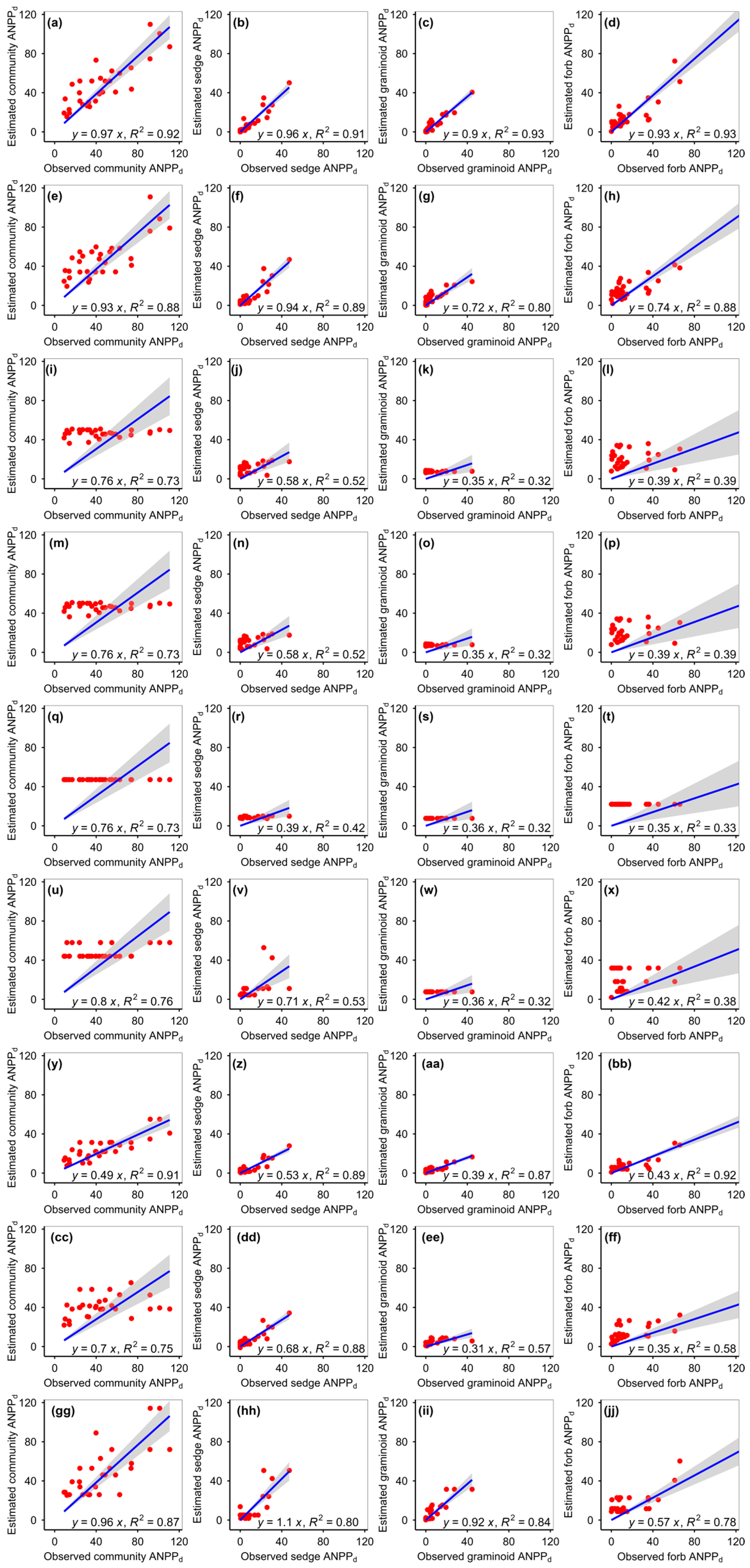
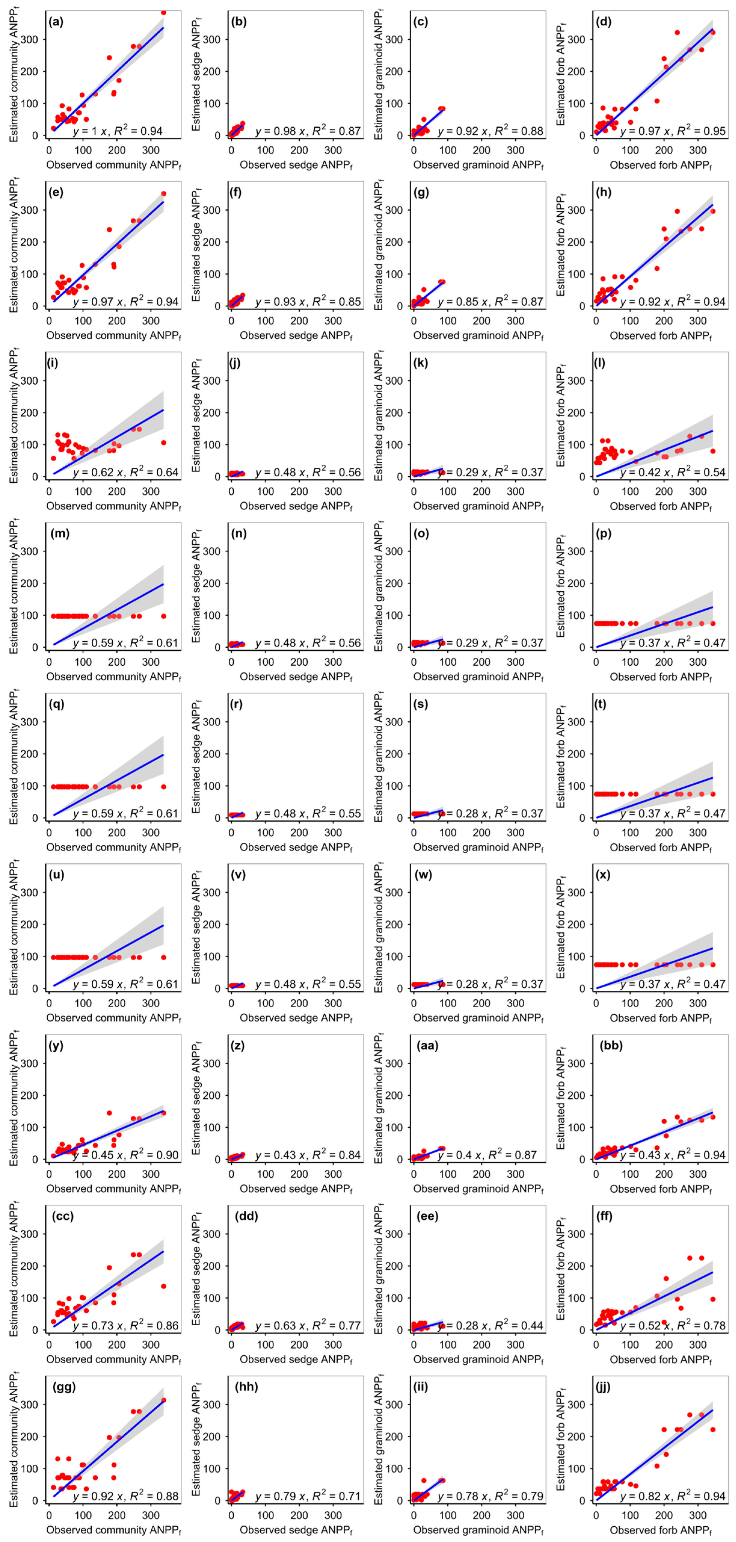
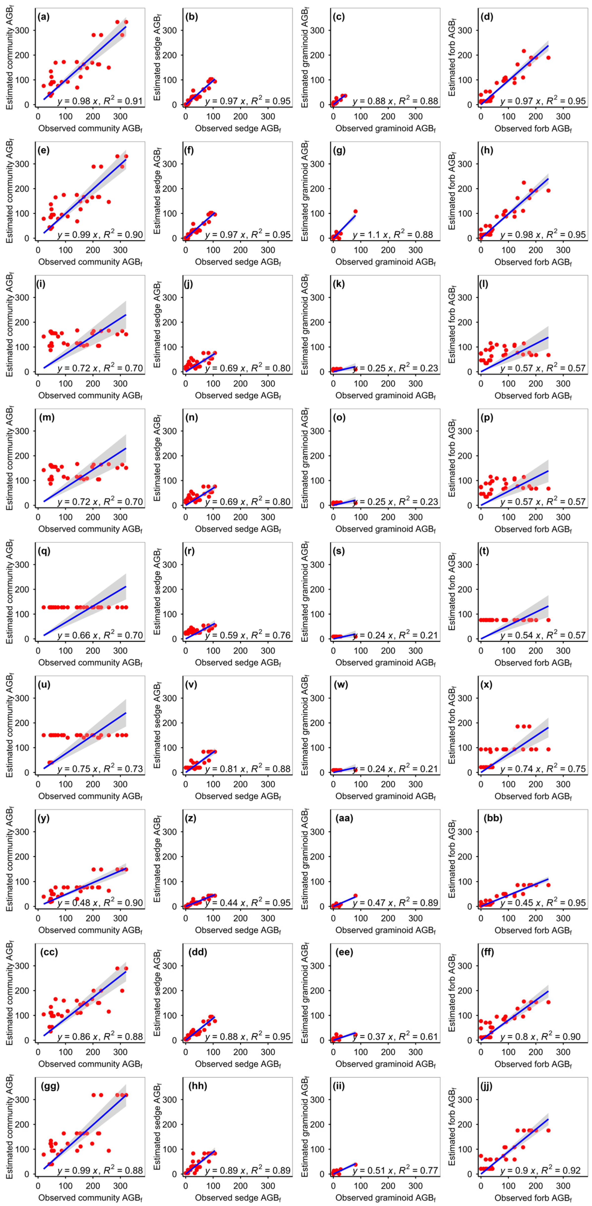
The RFM can have the highest accuracies considering its lower RMSE and absolute value of relative bias, and higher R² values between simulated and observed AGB or ANPP (Figure 2, Figure 3, Figure 4 and Figure 5,

Table 1. The relative bias (%) between estimated and observed fresh and dry aboveground net primary production under fencing conditions (ANPP_f and ANPP_d), and fresh and dry aboveground biomass (AGB_f and AGB_d) under grazing conditions of plant community, sedge, graminoid, and forb.

Condition	Variable	RFM	GBRM	MLRM	ANNM	GLRM	CITM	eXGBM	SVMM	RRTM
Fencing	Community ANPPf	0.99	0.45	−3.61	−4.17	−4.17	−4.17	−52.08	−13.92	1.40
	Community ANPPd	6.62	6.80	4.22	4.22	5.37	7.63	−45.39	−8.72	7.26
	Sedge ANPPf	3.26	4.61	−15.38	−15.38	−13.01	−13.01	−50.43	−17.62	−4.28
	Sedge ANPPd	−0.32	3.43	18.16	18.16	−2.51	8.76	−44.83	−23.11	19.58
	Graminoid ANPPf	−2.26	−5.47	−23.33	−23.33	−24.35	−24.35	−53.59	−43.61	−3.04
	Graminoid ANPPd	4.54	7.36	10.12	10.12	11.90	11.90	−48.09	−41.19	14.90
	Forb ANPPf	2.07	0.98	−20.03	−21.84	−21.84	−21.84	−53.20	−33.99	−7.68
	Forb ANPPd	0.37	−3.38	−0.44	−0.44	5.87	5.71	−51.55	−30.78	−11.75
Grazing	Community AGBf	7.43	8.74	0.32	0.32	−5.93	1.98	−47.34	1.68	9.67
	Community AGBd	3.93	0.55	26.64	26.64	17.69	20.28	−48.71	4.34	14.17
	Sedge AGBf	−2.67	−2.48	−13.38	−13.38	−16.79	−9.02	−54.35	−7.52	−4.36
	Sedge AGBd	−4.72	−6.05	−12.95	−12.95	−12.86	−8.28	−52.86	−34.20	2.66
	Graminoid AGBf	3.59	3.64	13.64	13.63	13.99	13.99	−51.07	−32.75	−16.00
	Graminoid AGBd	1.59	−1.83	−2.31	−2.31	−1.93	−14.50	−49.48	−27.65	−9.61
	Forb AGBf	3.07	2.53	−4.98	−4.98	−5.06	−5.16	−52.31	−3.68	−0.18
	Forb AGBd	−7.66	−7.25	−27.95	−27.95	−30.76	−24.37	−55.66	−45.96	−19.17

RFM, random forest model; GBRM, generalized boosted regression model; MLRM, multiple linear regression model; SVMM, support vector machine model; RRTM, recursive regression tree model; ANNM, artificial neural network model; GLRM, generalized linear regression model; CITM, conditional inference tree model; eXGBM, eXtreme gradient boosting model.

and

Table 2. The RMSE (g m⁻²) between estimated and observed fresh and dry aboveground net primary production under fencing conditions (ANPP_f and ANPP_d), and fresh and dry aboveground biomass (AGB_f and AGB_d) under grazing conditions of plant community, sedge, graminoid, and forb.

Condition	Variable	RFM	GBRM	MLRM	ANNM	GLRM	CITM	eXGBM	SVMM	RRTM
Fencing	Community ANPPf	31.45	32.07	77.62	80.84	80.84	80.84	73.82	51.96	45.05
	Comumnity ANPPd	15.41	18.20	27.25	27.25	27.66	26.03	28.05	26.45	19.46
	Sedge ANPPf	5.18	5.57	9.33	9.33	9.40	9.40	8.42	7.01	7.53
	Sedge ANPPd	4.48	4.91	10.19	10.19	11.21	10.79	7.42	5.91	7.79
	Graminoid ANPPf	9.41	9.76	21.54	21.54	21.58	21.58	16.54	20.91	12.18
	Graminoid ANPPd	3.27	5.53	9.92	9.92	9.95	9.95	7.52	131.07	5.00
	Forb ANPPf	32.16	32.81	96.82	103.30	103.30	103.30	80.99	76.21	38.02
	Forb ANPPd	9.74	13.69	28.26	28.26	29.58	28.48	21.23	124.76	19.05
Grazing	Community AGBf	51.02	52.05	87.80	87.80	88.61	83.77	88.40	56.69	59.13
	Community AGBd	17.51	16.76	30.87	30.87	27.69	26.66	27.47	24.78	18.77
	Sedge AGBf	10.90	11.10	23.30	23.30	26.87	18.25	28.70	12.03	17.10
	Sedge AGBd	6.26	5.75	12.78	12.78	12.63	12.29	11.04	12.11	7.45
	Graminoid AGBf	4.62	7.80	15.52	15.52	15.69	15.69	9.69	12.25	9.91
	Graminoid AGBd	1.56	2.15	4.23	4.23	4.02	3.69	3.31	4.33	3.18
	Forb AGBf	24.50	24.26	69.47	69.47	70.08	53.10	59.60	35.87	30.06
	Forb AGBd	8.73	9.35	26.70	26.70	27.84	25.21	21.56	25.26	15.31

RFM, random forest model; GBRM, generalized boosted regression model; MLRM, multiple linear regression model; SVMM, support vector machine model; RRTM, recursive regression tree model; ANNM, artificial neural network model; GLRM, generalized linear regression model; CITM, conditional inference tree model; eXGBM, eXtreme gradient boosting model.

). By contrast, the eXGBM can have the lowest accuracies (Figure 2, Figure 3, Figure 4 and Figure 5, Table 1 and Table 2).

4. Discussion

The eXGBM showed promising performance during training, but encountered notable errors during model validation (Table 1 and Table 2, and Table S6, Figure 2, Figure 3, Figure 4 and Figure 5). This phenomenon suggested potential overfitting of the eXGBM, wherein it performed well on the training data but poorly on the validation data. This emphasized the necessity of rigorous model validation procedures in future research to guarantee the model’s generalizability and reliability.

The RFM exhibited superior performance in predicting AGB at both the plant community and taxonomic group levels, as well as under both dry weight and fresh weight (Figure 2, Figure 3, Figure 4 and Figure 5, Table 1 and Table 2), possibly due to its enhanced robustness [35,36] (the ability to handle imbalanced and high-dimensional feature data) in handling outliers and noisy data compared to other models. Additionally, given the intricate relationships between specific taxonomic groups and variables, the RFM demonstrated proficiency in capturing these complexities. Unlike other models, RFM construction involves two critical parameters (ntree: number of trees and mtry: number of variables for splitting), for which this study identified optimal settings (Table S1), likely contributing to its heightened accuracy. Essentially, the RFM developed in this study not only shows promise in plant community AGB prediction but also displays comparable (even superior) performance in quantifying grassland AGB at the taxonomic group level.

The prediction accuracies of the RFM were different among the three taxonomic groups (Table 1 and Table 2, and Table S1, Figure 2, Figure 3, Figure 4 and Figure 5). This may be attributed to the varying effects of different taxonomic groups on the interpretation of satellite-based NDVI data [37]. Plant reflectance in the infrared spectrum can be negatively correlated with chlorophyll concentration, while plant reflectance in the near-infrared spectrum can be positively correlated with leaf area index [38,39]. Different plant taxonomic groups can exhibit different chlorophyll concentrations and leaf area indices [40]. For example, graminoid plants can have relatively low chlorophyll concentrations and leaf area indices [37]. In fact, the NDVI_max values of graminoid plants may be higher than those interpreted from remote sensing data. The relationships between different plant taxonomic groups and NDVI_max may vary, potentially explaining why the correlations between forb plants and NDVI_max can be stronger compared to sedge and graminoid plants. However, these differences could also stem from missing values in some quadrats [41], resulting in reduced prediction accuracies of the RFM models. Consequently, by calculating the difference in AGB between plant community and forb taxonomic group, it may be possible to indirectly assess the aboveground biomass of high-quality forage grasses (sedge and graminoid) with high accuracy and low costs. This could provide a feasible approach for more accurate assessments of the livestock carrying capacity of alpine grasslands.

The accuracies of the RFM for fresh AGB or ANPP were different from those for dry AGB or ANPP (Table 1 and Table 2and Table S1, Figure 2, Figure 3, Figure 4 and Figure 5). This could be attributed to the fact that plant water content may have more direct relationships with climatic factors [42]. Prolonged drought can reduce plant water content, while ample precipitation can increase it. In other words, the relationships between AGB and environmental factors may be more straightforward for fresh weight, resulting in higher model accuracy. This also implies that increasing the number of variables for splitting in the RFM did not necessarily lead to higher accuracy. The RFM developed in this study exhibited comparable or even superior accuracies of fresh AGB compared to dry AGB, suggesting that evaluating grassland fresh AGB may be feasible and have more direct implications for pastoralism.

The accuracies of the RFM under grazing conditions were not always higher than those under fencing conditions (Table 1 and Table 2, and Table S1, Figure 2, Figure 3, Figure 4 and Figure 5). This suggests that the inclusion of NDVI_max did not necessarily enhance model accuracy and may have even diminished it. Increasing the number of predictor variables can lead to higher data dimensionality, resulting in sparser data points in high-dimensional space [43,44], which may destabilize the model during training and generalization, thereby affecting its accuracy. Moreover, this situation could be attributed to the limited accuracy of NDVI_max [37], particularly in the Tibetan region, where cloud cover and rugged terrain may hinder the detection of certain changes by remote sensing imagery. In essence, incorporating predictor variables with low accuracy may inadvertently decrease model accuracy. Therefore, when developing models for quantifying AGB, it is crucial to comprehensively consider factors such as model complexity, generalization capability, computational resources, and data characteristics, and even conduct comparative analyses to select suitable predictor variables [44]. On the other hand, it should be noted that plant aboveground biomass measurements under grazing and fencing conditions were obtained from different datasets, which may also influence the results and require further investigation.

Previous studies have attempted to model and predict plant community AGB in the Tibetan grasslands, and some findings suggested that RFM was the optimal model for AGB prediction in this region [9,45]. However, the RFM developed in this study achieved comparable or even superior prediction accuracy (R² ≥ 0.87) for both AGB and ANPP using fewer predictor variables compared to previous studies (R² ≤ 0.88). This improvement could be attributed to the distinction made between enclosed and grazed areas in this study, likely contributing to higher model accuracy. Furthermore, the optimization of RFM parameters (ntree, mtry) in this study diverged from default values, potentially enhancing the accuracy of the RFM that was developed. These findings suggested that the RFM developed in this study effectively reduced model complexity, offering a novel approach to simplifying models for quantifying grassland AGB on the Tibetan Plateau.

However, this study had several limitations. For instance, the forb taxonomic groups did not distinguish between edible and inedible species, limiting the possibility of further evaluating the carrying capacity of Tibetan grasslands for livestock. Therefore, future research could focus on distinguishing the forb taxonomic groups further to provide better guidance for pastoralism development. Nonetheless, the RFM constructed for AGB quantification in this study can be used to quantify the impacts of climate change and human activities on AGB, as well as the spatial and temporal distribution of AGB water content. Additionally, by considering AGB not only at the plant community scale but also at the taxonomic group scale, this study offered a new perspective for more accurately quantifying the carrying capacity of Tibetan grasslands for livestock.

5. Conclusions

This study utilized nine models to model and validate the AGB of grassland communities and taxonomic groups (sedge, graminoid, and forb) under both enclosed and grazed conditions in Xizang’s grasslands, considering both dry weight and fresh weight. The RFM exhibited the highest accuracy among the nine models and performed comparably to previous studies. Furthermore, the RFM showed different accuracies among the three taxonomic groups and between dry weight and fresh weight. Therefore, this study actually can provide a new perspective for investigating the spatial distributions of grassland AGB on the Tibetan Plateau and even potentially on a global scale, as well as related studies on livestock carrying capacity.

References

1. O’Mara, F.P. The role of grasslands in food security and climate change. Ann. Bot. 2012, 110, 1263–1270. [Google Scholar] [CrossRef] [PubMed]
2. Guo, X.W.; Zhou, H.K.; Dai, L.C.; Li, J.; Zhang, F.W.; Li, Y.K.; Lin, L.; Li, Q.; Qian, D.W.; Fan, B.; et al. Restoration of Degraded Grassland Significantly Improves Water Storage in Alpine Grasslands in the Qinghai-Tibet Plateau. Front. Plant Sci. 2021, 12, 778656. [Google Scholar] [CrossRef]
3. Liu, Y.; Zhao, L.R.; Liu, Y.F.; Huang, Z.; Shi, J.J.; Wang, Y.L.; Ma, Y.S.; Lucas-Borja, M.E.; López-Vicente, M.; Wu, G.L. Restoration of a hillslope grassland with an ecological grass species (Elymus tangutorum) favors rainfall interception and water infiltration and reduces soil loss on the Qinghai-Tibetan Plateau. Catena 2022, 219, 106632. [Google Scholar] [CrossRef]
4. Lee, M.; Manning, P.; Rist, J.; Power, S.A.; Marsh, C. A global comparison of grassland biomass responses to CO2 and nitrogen enrichment. Philos. Trans. R. Soc. B-Biol. Sci. 2010, 365, 2047–2056. [Google Scholar] [CrossRef]
5. Dong, S.K.; Shang, Z.H.; Gao, J.X.; Boone, R.B. Enhancing sustainability of grassland ecosystems through ecological restoration and grazing management in an era of climate change on Qinghai-Tibetan Plateau. Agr. Ecosyst. Environ. 2020, 287, 106684. [Google Scholar] [CrossRef]
6. Borsellino, V.; Schimmenti, E.; El Bilali, H. Agri-Food Markets towards Sustainable Patterns. Sustainability 2020, 12, 2193. [Google Scholar] [CrossRef]
7. Salter, A.M.; Lopez-Viso, C. Role of novel protein sources in sustainably meeting future global requirements. Proc. Nutr. Soc. 2021, 80, 186–194. [Google Scholar] [CrossRef]
8. Flachowsky, G.; Meyer, U.; Südekum, K.H. Land Use for Edible Protein of Animal Origin-A Review. Animals 2017, 7, 25. [Google Scholar] [CrossRef]
9. Zeng, N.; Ren, X.L.; He, H.L.; Zhang, L.; Zhao, D.; Ge, R.; Li, P.; Niu, Z.E. Estimating grassland aboveground biomass on the Tibetan Plateau using a random forest algorithm. Ecol. Indic. 2019, 102, 479–487. [Google Scholar] [CrossRef]
10. Morais, T.G.; Teixeira, R.F.M.; Figueiredo, M.; Domingos, T. The use of machine learning methods to estimate aboveground biomass of grasslands: A review. Ecol. Indic. 2021, 130, 108081. [Google Scholar] [CrossRef]
11. Yao, X.; Chai, Q.; Chen, T.X.; Chen, Z.J.; Wei, X.K.; Bao, G.S.; Song, M.L.; Wei, W.R.; Zhang, X.X.; Li, C.J.; et al. Disturbance by grazing and the presence of rodents facilitates the dominance of the unpalatable grass Achnatherum inebrians in alpine meadows of northern China. Rangel. J. 2019, 41, 301–312. [Google Scholar] [CrossRef]
12. Zhao, M.L.; Gao, X.L.; Wang, J.; He, X.L.; Han, B. A review of the most economically important poisonous plants to the livestock industry on temperate grasslands of China. J. Appl. Toxicol. 2013, 33, 9–17. [Google Scholar] [CrossRef] [PubMed]
13. Han, F.; Yu, C.; Fu, G. Non-growing/growing season non-uniform-warming increases precipitation use efficiency but reduces its temporal stability in an alpine meadow. Front. Plant Sci. 2023, 14, 1090204. [Google Scholar] [CrossRef] [PubMed]
14. Chen, X.; Luo, M.Y.; Larjavaara, M. Effects of climate and plant functional types on forest above-ground biomass accumulation. Carbon Balance Manag. 2023, 18, 5. [Google Scholar] [CrossRef] [PubMed]
15. Zeng, N.; Ren, X.L.; He, H.L.; Zhang, L.; Li, P.; Niu, O.G. Estimating the grassland aboveground biomass in the Three-River Headwater Region of China using machine learning and Bayesian model averaging. Environ. Res. Lett. 2021, 16, 114020. [Google Scholar] [CrossRef]
16. Wang, G.Q.; Liu, S.M.; Liu, T.X.; Fu, Z.Y.; Yu, J.S.; Xue, B.L. Modelling above-ground biomass based on vegetation indexes: A modified approach for biomass estimation in semi-arid grasslands. Int. J. Remote Sens. 2019, 40, 3835–3854. [Google Scholar] [CrossRef]
17. Ma, X.L.; Ma, Y.J. The spatiotemporal variation analysis of virtual water for agriculture and livestock husbandry: A study for Jilin Province in China. Sci. Total Environ. 2017, 586, 1150–1161. [Google Scholar] [CrossRef] [PubMed]
18. Leng, G.Y.; Hall, J.W. Where is the Planetary Boundary for freshwater being exceeded because of livestock farming? Sci. Total Environ. 2021, 760, 144035. [Google Scholar] [CrossRef] [PubMed]
19. Wei, Y.Q.; Wang, S.J.; Fang, Y.P.; Nawaz, Z. Integrated assessment on the vulnerability of animal husbandry to snow disasters under climate change in the Qinghai-Tibetan Plateau. Glob. Planet. Change 2017, 157, 139–152. [Google Scholar] [CrossRef]
20. Wen, L.; Dong, S.K.; Li, Y.Y.; Pulver, C.; Li, X.Y.; Shi, J.J.; Wang, Y.L.; Ma, Y.S.; Liu, D.M. Variation of botanical composition, forage production and nutrient values along a grassland degradation gradient in the alpine region of Qinghai-Tibet Plateau. Phyton-Int. J. Exp. Bot. 2013, 82, 45–54. [Google Scholar]
21. Gao, X.X.; Dong, S.K.; Li, S.; Xu, Y.D.; Liu, S.L.; Zhao, H.D.; Yeomans, J.; Li, Y.; Shen, H.; Wu, S.N.; et al. Using the random forest model and validated MODIS with the field spectrometer measurement promote the accuracy of estimating aboveground biomass and coverage of alpine grasslands on the Qinghai-Tibetan Plateau. Ecol. Indic. 2020, 112, 106114. [Google Scholar] [CrossRef]
22. Jia, Z.Y.; Zhang, Z.H.; Cheng, Y.X.; Buhebaoyin; Borjigin, S.; Quan, Z.J. Grassland biomass spatiotemporal patterns and response to climate change in eastern Inner Mongolia based on XGBoost model estimates. Ecol. Indic. 2024, 158, 111554. [Google Scholar] [CrossRef]
23. Pham, T.D.; Le, N.N.; Ha, N.T.; Nguyen, L.V.; Xia, J.S.; Yokoya, N.; To, T.T.; Trinh, H.X.; Kieu, L.Q.; Takeuchi, W. Estimating Mangrove Above-Ground Biomass Using Extreme Gradient Boosting Decision Trees Algorithm with Fused Sentinel-2 and ALOS-2 PALSAR-2 Data in Can Gio Biosphere Reserve, Vietnam. Remote Sens. 2020, 12, 777. [Google Scholar] [CrossRef]
24. Tian, Y.; Fu, G. Quantifying Plant Species α-Diversity Using Normalized Difference Vegetation Index and Climate Data in Alpine Grasslands. Remote Sens. 2022, 14, 5007. [Google Scholar] [CrossRef]
25. Wang, S.H.; Fu, G. Modelling soil moisture using climate data and normalized difference vegetation index based on nine algorithms in alpine grasslands. Front. Environ. Sci. 2023, 11, 1130448. [Google Scholar] [CrossRef]
26. Huang, S.; Fu, G. Impacts of climate change and human activities on plant species α-diversity across the Tibetan grasslands. Remote Sens. 2023, 15, 2947. [Google Scholar] [CrossRef]
27. Ran, Q.W.; Hao, Y.B.; Xia, A.Q.; Liu, W.J.; Hu, R.H.; Cui, X.Y.; Xue, K.; Song, X.N.; Xu, C.; Ding, B.Y.; et al. Quantitative Assessment of the Impact of Physical and Anthropogenic Factors on Vegetation Spatial-Temporal Variation in Northern Tibet. Remote Sens. 2019, 11, 1183. [Google Scholar] [CrossRef]
28. Chen, Y.; Xu, E. The Spatiotemporal Change in Land Cover and Discrepancies within Different Countries on the Qinghai-Tibet Plateau over a Recent 30-Year Period. Land 2023, 12, 1797. [Google Scholar] [CrossRef]
29. Ding, J.Z.; Yang, T.; Zhao, Y.T.; Liu, D.; Wang, X.Y.; Yao, Y.T.; Peng, S.S.; Wang, T.; Piao, S.L. Increasingly Important Role of Atmospheric Aridity on Tibetan Alpine Grasslands. Geophys. Res. Lett. 2018, 45, 2852–2859. [Google Scholar] [CrossRef]
30. Yang, J.; Dong, J.; Xiao, X.; Dai, J.; Wu, C.; Xia, J.; Zhao, G.; Zhao, M.; Li, Z.; Zhang, Y.; et al. Divergent shifts in peak photosynthesis timing of temperate and alpine grasslands in China. Remote Sens. Environ. 2019, 233, 111395. [Google Scholar] [CrossRef]
31. Fu, G.; Sun, W.; Li, S.W.; Zhang, J.; Yu, C.Q.; Shen, Z.X. Modeling aboveground biomass using MODIS images and climatic data in grasslands on the Tibetan Plateau. J. Resour. Ecol. 2017, 8, 42–49. [Google Scholar]
32. Zhang, G.; Fu, G. Changes in soil organic carbon, total nitrogen and total phosphorus in 2000–2020 and their driving mechanisms in Tibetan alpine grasslands. Glob. Planet. Chang. 2024, 239, 104484. [Google Scholar] [CrossRef]
33. Han, F.; Fu, G.; Yu, C.; Wang, S. Modeling nutrition quality and storage of forage using climate data and normalized-difference vegetation index in alpine grasslands. Remote Sens. 2022, 14, 3410. [Google Scholar] [CrossRef]
34. Sun, W.; Qi, H.; Li, T.; Qin, Y.; Fu, G.; Han, F.; Wang, S.; Pan, X. Modelling soil ammonium nitrogen, nitrate nitrogen and available phosphorus using normalized difference vegetation index and climate data in Xizang’s grasslands. Sustainability 2024, 16, 4695. [Google Scholar] [CrossRef]
35. Rodriguez-Galiano, V.; Sanchez-Castillo, M.; Chica-Olmo, M.; Chica-Rivas, M. Machine learning predictive models for mineral prospectivity: An evaluation of neural networks, random forest, regression trees and support vector machines. Ore Geol. Rev. 2015, 71, 804–818. [Google Scholar] [CrossRef]
36. Wang, L.A.; Zhou, X.D.; Zhu, X.K.; Dong, Z.D.; Guo, W.S. Estimation of biomass in wheat using random forest regression algorithm and remote sensing data. Crop J. 2016, 4, 212–219. [Google Scholar] [CrossRef]
37. Wang, H.; Liu, H.Y.; Huang, N.; Bi, J.; Ma, X.L.; Ma, Z.Y.; Shangguan, Z.J.; Zhao, H.F.; Feng, Q.S.; Liang, T.G.; et al. Satellite-derived NDVI underestimates the advancement of alpine vegetation growth over the past three decades. Ecology 2021, 102, e03518. [Google Scholar] [CrossRef]
38. Peñuelas, J.; Filella, I. Visible and near-infrared reflectance techniques for diagnosing plant physiological status. Trends Plant Sci. 1998, 3, 151–156. [Google Scholar] [CrossRef]
39. Colwell, J.E. Vegetation canopy reflectance. Remote Sens. Environ. 1974, 3, 175–183. [Google Scholar] [CrossRef]
40. Dubey, P.; Raghubanshi, A.S.; Singh, J.S. Intra-seasonal variation and relationship among leaf traits of different forest herbs in a dry tropical environment. Curr. Sci. 2011, 100, 69–76. [Google Scholar]
41. Yang, Y.; Klanderud, K.; Yang, Y.H.; Jin, H.A.; Lu, Y.Q.; Zhang, T.Z.; Wang, G.X. Homogenization in Species Composition and No Change in Aboveground Biomass Across Tibetan Permafrost Regions Over Ten Years. Front. Environ. Sci. 2022, 10, 932993. [Google Scholar] [CrossRef]
42. Wang, L.T.; Wang, S.X.; Zhou, Y.; Liu, W.L.; Wang, F.T. Vegetation Water Content Retrieval and Application of Drought Monitoring Using Multi-Spectral Remote Sensing. Spectrosc. Spectr. Anal. 2011, 31, 2804–2808. [Google Scholar] [CrossRef]
43. Yu, Q.Y.; Ji, W.J.; Prihodko, L.; Ross, C.W.; Anchang, J.Y.; Hanan, N.P. Study becomes insight: Ecological learning from machine learning. Methods Ecol. Evol. 2021, 12, 2117–2128. [Google Scholar] [CrossRef]
44. Cappart, Q.; Bergman, D.; Rousseau, L.M.; Prémont-Schwarz, I.; Parjadis, A. Improving Variable Orderings of Approximate Decision Diagrams Using Reinforcement Learning. Inf. J. Comput. 2022, 34, 2552–2570. [Google Scholar] [CrossRef]
45. Fan, X.Y.; He, G.J.; Zhang, W.Y.; Long, T.F.; Zhang, X.M.; Wang, G.Z.; Sun, G.; Zhou, H.K.; Shang, Z.H.; Tian, D.S.; et al. Sentinel-2 Images Based Modeling of Grassland Above-Ground Biomass Using Random Forest Algorithm: A Case Study on the Tibetan Plateau. Remote Sens. 2022, 14, 5321. [Google Scholar] [CrossRef]
Figure 1. Sampling sites and meteorological stations.
Agronomy 14 01515 g001
Figure 2. Comparison of dry weight of estimated and observed aboveground net primary production (ANPPd) of plant community, sedge, graminoid, and forb for (ad) RFM, (eh) GBRM, (il) MLRM, (mp) ANNM, (qt) GLRM, (ux) CITM, (ybb) eXGBM, (ccff) SVMM, and (ggjj) RRTM under fencing conditions. The solid lines are the linear regression between the estimated and observed ANPPd. RFM, random forest model; GBRM, generalized boosted regression model; MLRM, multiple linear regression model; SVMM, support vector machine model; RRTM, recursive regression tree model; ANNM, artificial neural network model; GLRM, generalized linear regression model; CITM, conditional inference tree model; eXGBM, eXtreme gradient boosting model.
Agronomy 14 01515 g002
Figure 3. Comparison of dry weight of estimated and observed aboveground biomass (AGBd) of plant community, sedge, graminoid, and forb for (ad) RFM, (eh) GBRM, (il) MLRM, (mp) ANNM, (qt) GLRM, (ux) CITM, (ybb) eXGBM, (ccff) SVMM, and (ggjj) RRTM under grazing conditions. The solid lines are the linear regression between the estimated and observed AGBd. RFM, random forest model; GBRM, generalized boosted regression model; MLRM, multiple linear regression model; SVMM, support vector machine model; RRTM, recursive regression tree model; ANNM, artificial neural network model; GLRM, generalized linear regression model; CITM, conditional inference tree model; eXGBM, eXtreme gradient boosting model.
Agronomy 14 01515 g003
Figure 4. Comparison of fresh weight of estimated and observed aboveground net primary production (ANPPf) of plant community, sedge, graminoid, and forb for (ad) RFM, (eh) GBRM, (il) MLRM, (mp) ANNM, (qt) GLRM, (ux) CITM, (ybb) eXGBM, (ccff) SVMM, and (ggjj) RRTM under fencing conditions. The solid lines are the linear regression between the estimated and observed ANPPf. RFM, random forest model; GBRM, generalized boosted regression model; MLRM, multiple linear regression model; SVMM, support vector machine model; RRTM, recursive regression tree model; ANNM, artificial neural network model; GLRM, generalized linear regression model; CITM, conditional inference tree model; eXGBM, eXtreme gradient boosting model.
Agronomy 14 01515 g004
Figure 5. Comparison of fresh weight of estimated and observed aboveground biomass (AGBf) of plant community, sedge, graminoid, and forb for (ad) RFM, (eh) GBRM, (il) MLRM, (mp) ANNM, (qt) GLRM, (ux) CITM, (ybb) eXGBM, (ccff) SVMM, and (ggjj) RRTM under grazing conditions. The solid lines are the linear regression between the estimated and observed AGBf. RFM, random forest model; GBRM, generalized boosted regression model; MLRM, multiple linear regression model; SVMM, support vector machine model; RRTM, recursive regression tree model; ANNM, artificial neural network model; GLRM, generalized linear regression model; CITM, conditional inference tree model; eXGBM, eXtreme gradient boosting model.
Agronomy 14 01515 g005