Abstract
Pest damage is a major factor in reducing crop yield and has negative impacts on the economy. However, the complex background, diversity of pests, and individual differences pose challenges for classification algorithms. In this study, we propose a patch-based neural network (PMLPNet) for multi-class pest classification. PMLPNet leverages spatial and channel contextual semantic features through meticulously designed token- and channel-mixing MLPs, respectively. This innovative structure enhances the model’s ability to accurately classify complex multi-class pests by providing high-quality local and global pixel semantic features for the fully connected layer and activation function. We constructed a database of 4510 images spanning 40 types of plant pests across 4 crops. Experimental results demonstrate that PMLPNet outperforms existing CNN models, achieving an accuracy of 92.73%. Additionally, heat maps reveal distinctions among different pest images, while patch probability-based visualizations highlight heterogeneity within pest images. Validation on external datasets (IP102 and PlantDoc) confirms the robust generalization performance of PMLPNet. In summary, our research advances intelligent pest classification techniques, effectively identifying various pest types in diverse crop images.
1. Introduction
With the continuous growth of the world population, food security is a prerequisite for ensuring the normal operation of society and production. As is well known, the harm of pests accompanies the entire growth cycle of crops and is one of the main causes of global crop losses [1]. However, there are many types of crop pests. These pests typically manifest in different forms, including damage to leaves, stems, flowers, and fruits, and may even lead to virus transmission. According to data from the Food and Agriculture Organization of the United Nations, plant diseases cause over USD 220 billion in losses to the global economy every year. In addition, up to 40% of global crop production is lost annually due to pests, resulting in losses of at least USD 70 billion [2]. Therefore, preventing and controlling pests can not only improve food quality but also reduce agricultural losses, which is crucial for food security and stabilizing the agricultural economy [3]. The prerequisite for implementing this task is to accurately identify pest populations for precise pest control.
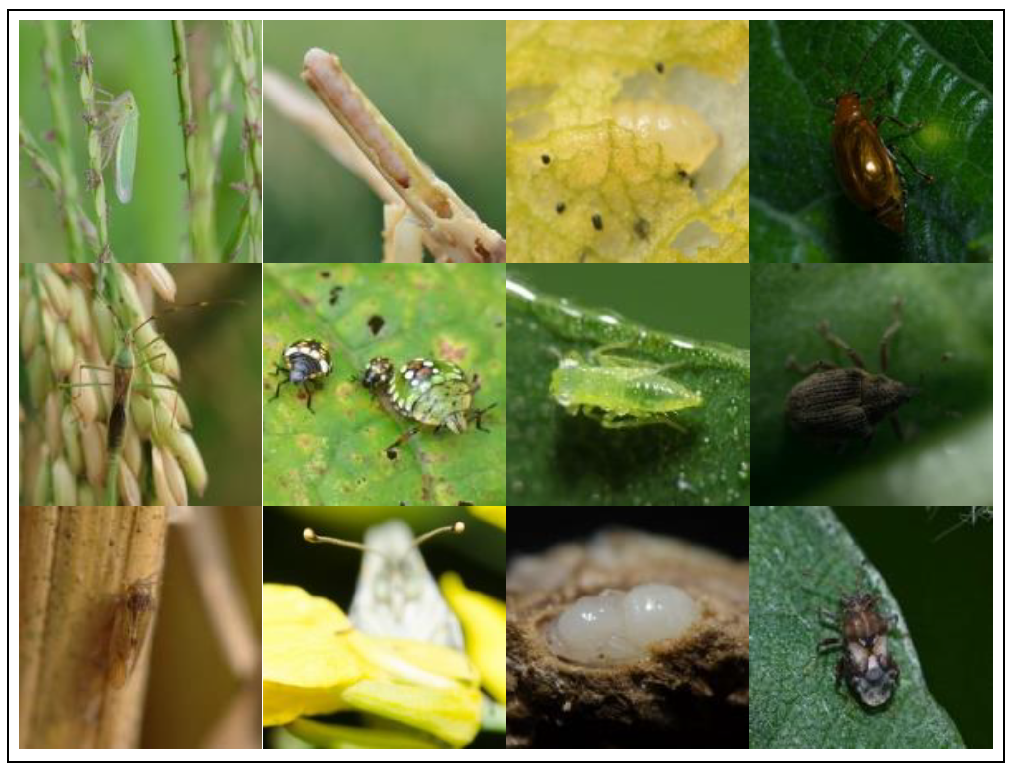
Currently, most methods for identifying crop pests and diseases mainly rely on manual observation or individual sample detection, which is a time-consuming and inefficient task. As shown in Figure 1, there are many types of pests, and there are subtle differences in the field environment. The accuracy and efficiency of pest identification mainly depend on the professional knowledge of agricultural experts. However, high-precision detection methods based on molecular detection are limited by centralized laboratories and expensive devices [4], and also rely on professional knowledge. In addition, the similarity and diversity of pests make accurate visual classification very difficult. The appearance and characteristics of pests may change with different stages of their life cycle, further increasing the difficulty of pest identification. Complex environmental factors also increase the difficulty of accurate identification.

Figure 1.
Example images of the pests. Each image belongs to a different species of pests.
In recent years, with the improvement of computer hardware performance, artificial intelligence (AI) technologies have achieved super performance in computer vision studies [5], such as object detection [6], medical imaging classification [7], lesion segmentation [8], cell image analysis [9], etc. This type of method not only achieves high accuracy but also decreases time and money consumption and provides a new way to analyze and identify crop pests.
As a representative of AI technology, deep convolutional neural networks (CNNs) are inspired by the working mode of animal vision systems, in which neurons perform local and in-depth processing of visual perception areas. CNN mainly includes the following important components: convolutional layer, pooling layer, activation function, and fully connected layer [10]. The main advantage of CNN lies in its processing efficiency for gridded data. By sharing parameters and gradually extracting features through hierarchical structures, CNN can capture local and global patterns in the data, making it perform well in image recognition and object detection [11]. CNN has made many important breakthroughs in the field of computer vision.
According to the survey [12], a depth separable CNN was trained on a public dataset that consists of 14 different plant species and 38 different categorical diseases and healthy plant leaves. This CNN model not only reduces the number of parameters and computational costs but also achieves an accuracy of 98.42%. Naik et al. [13] used 12 different pre-trained deep learning networks to identify 5 diseases from leaves, including leaf bending, gemini virus, cercospora leaf spot disease, yellow leaf disease, and upper leaf bending disease. Among them, the proposed SECNN achieved optimal accuracies of 99.12% and 98.63% with and without enhancement, respectively. In addition, a Faster R-CNN was proposed to detect rice leaf diseases [14], which was effective in automatic diagnosis of three discriminative rice leaf diseases: rice blast, brown spot, and hispa, with accuracy rates of 98.09%, 98.85%, and 99.17%, respectively. In addition, the model can recognize healthy rice leaves with an accuracy of 99.25%. These methods have promoted the study of plant types or crop disease classification to some extent, but these methods only show strong performance in one dataset or small sample size; the generalization ability of the model needs to be further verified.
In recent years, to solve the problem of limited sample size, many researchers have applied transfer learning technology to the study of crop pests [15,16]. This type of method typically uses the ImageNet dataset as the pre-training dataset, and then transfers the weights of the pre-training model to another task. For example, Paymode et al. [17] used the VGG-based transfer learning method to predict the types of diseases and pests in early grape and tomato leaves. The method has achieved an accuracy of 98.40% for grapes and 95.71% for tomatoes. Thangaraj et al. [18] proposed a deep CNN model to identify tomato leaf disease. Krishnamoorthy et al. [19] utilized the InceptionResNetV2 model to identify pests in rice leaf images, achieving an accuracy of 95.67%. Furthermore, residual and attention mechanisms are used for plant or agricultural pest disease detection and classification [20]. Liu et al. present a DCNN for the visual localization and classification of pests from paddy field images [21]. An unsupervised CNN method was developed for the classification of pest species in field crops, such as corn, soybeans, wheat, and rapeseed [22]. This method achieved the classification of 40 types of crop pests by learning the features of the images from a large number of unlabeled image blocks. Too et al. used DenseNets to classify leaf disease and health images of 14 plants in the PlantVillage dataset [23]. Although the above methods or mechanisms can improve the model’s attention to the target object, the limitations of CNN’s own feature acquisition still cannot be ignored. This is mainly caused by the locality of convolution operations.
The high efficiency of the transformer model in processing long sequences makes it a powerful model in the field of image analysis research. More and more researchers are applying this model to crop image studies. For example, Gu et al. [24] proposed a classification CNN model that combines shift window transformer blocks with lightweight CNN models. They applied a shift window transformer to the process of feature extraction to obtain global feature information. In addition, Cheng et al. [25] introduced a hybrid CNN transformer in the classification model. They used CNN and converters to extract spatial and channel feature information. Pereira et al. [26] improved the classification CNN structure by using spatially adaptive recalibration blocks (SegSE blocks). The SegSE block recalibrates the feature map by considering cross-channel information and spatial correlation, helping to obtain global and local feature information as proposed. Saranya et al. [27] proposed a modified ViT transformer model (HPMA), which emphasizes discriminative features and suppresses irrelevant info for robustness. HPMA was verified on three pest datasets and achieved good performance.
However, in pest classification tasks, most CNNs are limited to controlled laboratory environments, which cannot meet the requirements of pest identification in real outdoor environments. In addition, pest classification has its own characteristics that are different from natural image object classification work [28]. Specifically, compared with other plant disease classification studies, our study focuses solely on the classification of agricultural pests, rather than the identification of multiple types of plant diseases. Although many researchers focus on using machine learning, deep learning, and other methods to analyze and explore pest identification, they prefer to study a single pest classification rather than mixing multiple classifications of various types of pests together, which is common in published work. In addition, many pests are very similar in morphology, and there may be multiple different pests on crops. This makes accurate classification visually very difficult. The appearance and characteristics of pests may change with different stages of their life cycle, which increases the difficulty of classifying multiple types of pests. And this study is a classification study for various crops and pests involving a variety of species and complex environments, which is helpful for the practical significance of intelligent classification of pests in agricultural scenarios.
In the present study, we propose a patch-based neural network (PMLPNet) for multi-class pest classification. The main contributions are listed as follows:
- (1)
- PMLPNet is proposed for multi-class pest classification, which integrates local and global contextual semantic features by designed token- and channel-mixing MLP structures.
- (2)
- The patch-based image input strategy not only improves the performance of PMLPNet, but also provides a basis for image heterogeneity analysis.
- (3)
- The GELU activation function improves the ability of PMLPNet to fit complex data distributions and enhances the capabilities of PMLPNet.
2. Materials and Methods
2.1. Dataset and Preprocessing
Our data comes from two sources: One comes from agricultural pest websites; the pest images were extracted from several professional agricultural pest image and video websites. Another comes from Google and Baidu search engines, using both Chinese and English keywords to obtain the target image. Finally, we collected a pest dataset containing 6000 images of 40 pest types. These images consist of 4 types of crops, including corn, soybeans, wheat, and rapeseed. These images involve farmland and laboratory scenes, and there are significant differences in the sizes of the pests in the images.
In order to improve image quality, we organized 3 volunteers with knowledge of agricultural pests to manually filter candidate images. We deleted images with blurry scenes, high noise, or missing targets. Because pests in different life cycles can cause varying degrees of damage to agricultural products, we retained different forms of pests such as eggs, larvae, pupae, and adults. In addition, we also retained images of pests with different sizes, such as larger beetles and tine aphids. Finally, we obtained 4510 images with their labels. The details of the dataset are listed in Table 1. Note that these images are complex, including parts of crops, different backgrounds, ground textures, and shadow effects. Furthermore, the size difference of pests is also significant.
In order to meet the sample size requirements of deep learning models, we adopted data augmentation techniques to expand the dataset, including affine image transformation, diffusion models, random cropping, rotation, scaling, and horizontal flipping. Data augmentation significantly increases the diversity of data available for training models and improves the ability of classification models to learn appropriate features [29]. Finally, we obtained a dataset that consists of 22,550 images; this was created by combining the original images.
2.2. Overview of Our Method
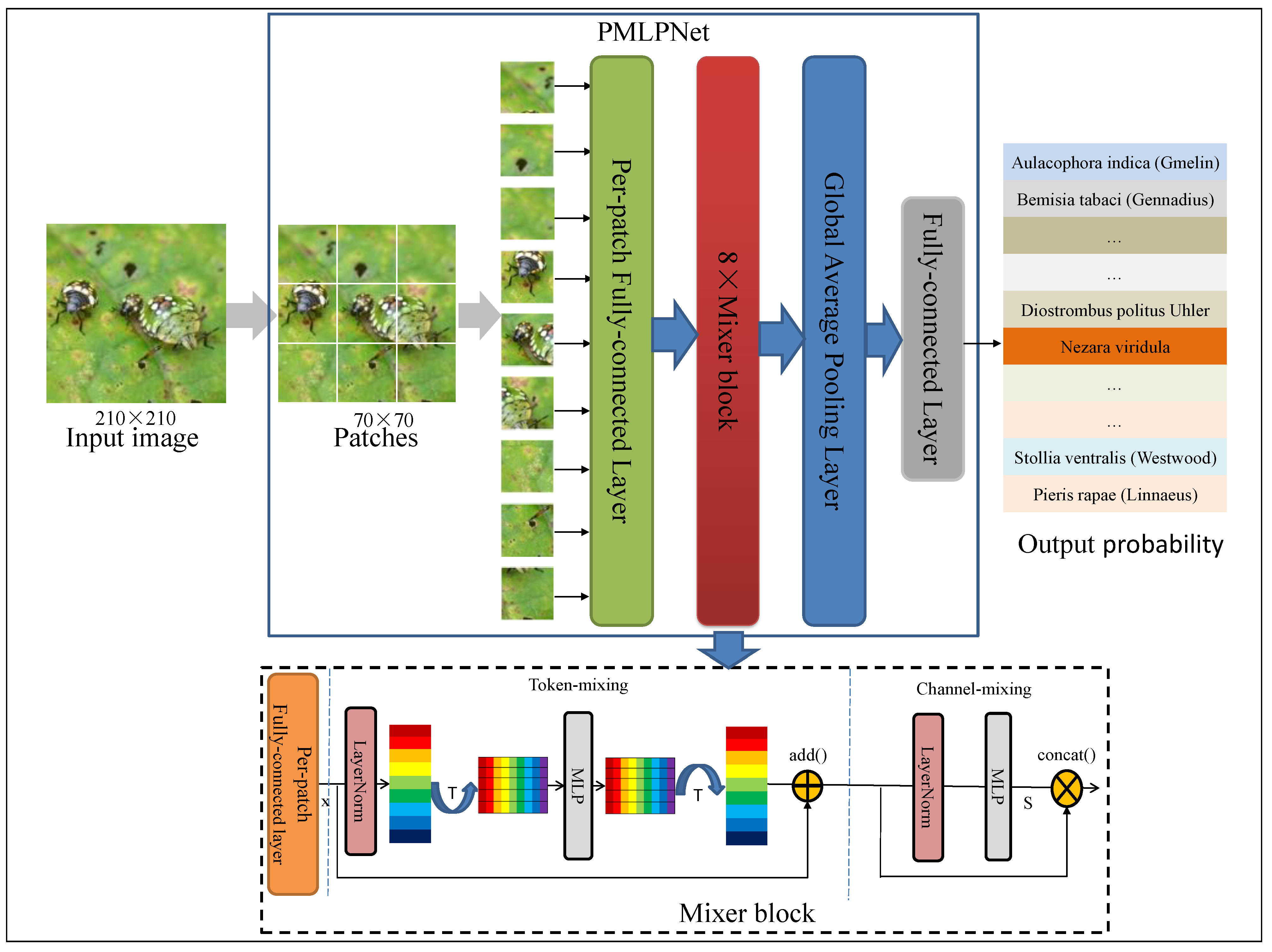
Figure 2 illustrates the pipeline of our proposed framework (PMLPNet). All precessed images are unified as 210 × 210 pixels. PMLPNet is used to extract contextual semantic information based on patches of an image. In PMLPNet, we adopted 8 mixer blocks to extract the spatial and channel features from patch-level images. Finally, image-level pest class prediction was completed by a fully connected layer and sigmoid activation function.
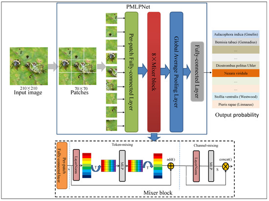
Figure 2.
The pipeline for the proposed PMLPNet. “T” is transposition operation, which is used to transpose feature maps.
In CNNs, the convolutional operation extracts the local features from an image, which has made significant progress in the field of image analysis. However, the neglected global features make it difficult for these methods to accurately identify the target when complex backgrounds, small target granularity, and similar targets are present. To overcome these limitations, in this study, we propose a patch-based multi-layer perceptron neural network (PMLPNet) for multi-class pest classification (as shown in Figure 2). Mixer block is a key part of PMLPNet, which integrates spatial contextual semantic features (i.e., the global capacity) and channel contextual semantic features (i.e., a local prior) by token- and channel-mixing MLPs, respectively. The details of mixer block are shown on the bottom of Figure 2. Mixer block offers the high-quality pixel positioning features for the fully connected layers and activation function, which helps the model to accurately classify pests.

Table 1.
The details of the pest dataset in our study.
Table 1.
The details of the pest dataset in our study.
| ID | Pest Names | Number | ID | Pest Names | Number | ID | Pest Names | Number | ID | Pest Names | Number |
|---|---|---|---|---|---|---|---|---|---|---|---|
| 1 | Aulacophora indica (Gmelin) | 78 | 11 | Corythucha ciliata (Say) | 90 | 21 | Halyomorpha halys (Stål) | 101 | 31 | Pieris rapae (Linnaeus) | 71 |
| 2 | Bemisia tabaci (Gennadius) | 147 | 12 | Corythucha marmorata(Uhler) | 98 | 22 | Iscadia inexacta (Walker) | 79 | 32 | Plutella xylostella (Linnaeus) | 69 |
| 3 | Callitettix versicolor (Fabricius) | 156 | 13 | Dicladispa armigera (Olivier) | 150 | 23 | Laodelphax striatellus (Fall en) | 61 | 33 | Porthesia taiwana Shiraki | 141 |
| 4 | Ceroplastes ceriferus (Anderson) | 100 | 14 | Diostrombus politus Uhler | 238 | 24 | Leptocorisa acuta (Thunberg) | 133 | 34 | Riptortus pedestris (Fabricius) | 110 |
| 5 | Ceutorhynchus asper Roelofs | 146 | 15 | Dolerus tritici Chu | 88 | 25 | Luperomorpha suturalis Chen | 101 | 35 | Scotinophara lurida (Burmeister) | 117 |
| 6 | Chauliops fallax Scott | 68 | 16 | Dolycoris baccarum (Linnaeus) | 87 | 26 | Lycorma delicatula (White) | 92 | 36 | Sesamia inferens (Walker) | 126 |
| 7 | Chilo supperssalis (Walker) | 93 | 17 | Dryocosmus KuriphilusYasumatsu | 50 | 27 | Maruca testulalis Gryer | 73 | 37 | Spilosoma obliqua (Walker) | 66 |
| 8 | Chromatomyia horticola(Goureau) | 114 | 18 | Empoasca flavescens (Fabricius) | 133 | 28 | Nezara viridula (Linnaeus) | 175 | 38 | Spodoptera litura (Fabricius) | 130 |
| 9 | Cicadella viridis (Linnaeus) | 138 | 19 | Eurydema dominulus (Scopoli) | 150 | 29 | Nilaparvata lugens (Stål) | 62 | 39 | Stollia ventralis (Westwood) | 72 |
| 10 | Cletus punctiger (Dallas) | 169 | 20 | Graphosoma rubrolineata (Westwood) | 116 | 30 | Phyllotreta striolata (Fabricius) | 187 | 40 | Strongyllodes variegatus (Fairmaire) | 135 |
Generally, CNNs obtain the contextual semantic features of a pixel from the input image through the convolution operation and make predictions. Due to the localization of the convolution operation, each pixel is closely related to the adjacent pixels and has a weaker relationship with distant pixels. This poses a challenge for identifying small-sized pests from complex background images. We address these problems by adopting spatial and channel contextual semantic optimization. Specifically, the spatial contextual semantic features are obtained from the transposed feature maps in the token-mixing MLP, and the channel contextual semantic features are obtained from the feature maps through the convolution operation in the channel-mixing MLP [30]. As shown in Figure 2, an image is input into PMLPNet and divided into 9 patches with pixels, which are fed into the backbone of PMLPNet. PMLPNet consists of 8 token and channel mixer blocks. The global average pooling layer and fully connected layer follow the mixer blocks. Finally, the prediction probability of pest species is output by the activation function.
The pipeline of the proposed mixer block is shown in Figure 2. There are 8 mixer blocks in PMLPNet. A mixer block is composed of token- and channel-mixing MLPs. Token-mixing consists of a LayerNorm, transpose operation, MLP, transpose operation, and skip-connection layer. The output of token-mixing is generated by fusing the fully connected layer output and the input of token-mixing by the skip-connection operation (). Similarly, channel-mixing also undergoes the same structure and feature output strategy as token-mixing. Finally, to fuse global and local features, we use skip-connection to combine the output features of token- and channel-mixing along the channel dimension. In the mixer block, the token-mixing MLP facilitates communication among various spatial positions (tokens) to fuse spatial domain information. On the other hand, the channel-mixing MLP facilitates communication among different channels to fuse channel domain information. After each mixer block, we use dropout regularization to reduce the overfitting problem and reduce features to reduce dependencies between neurons.
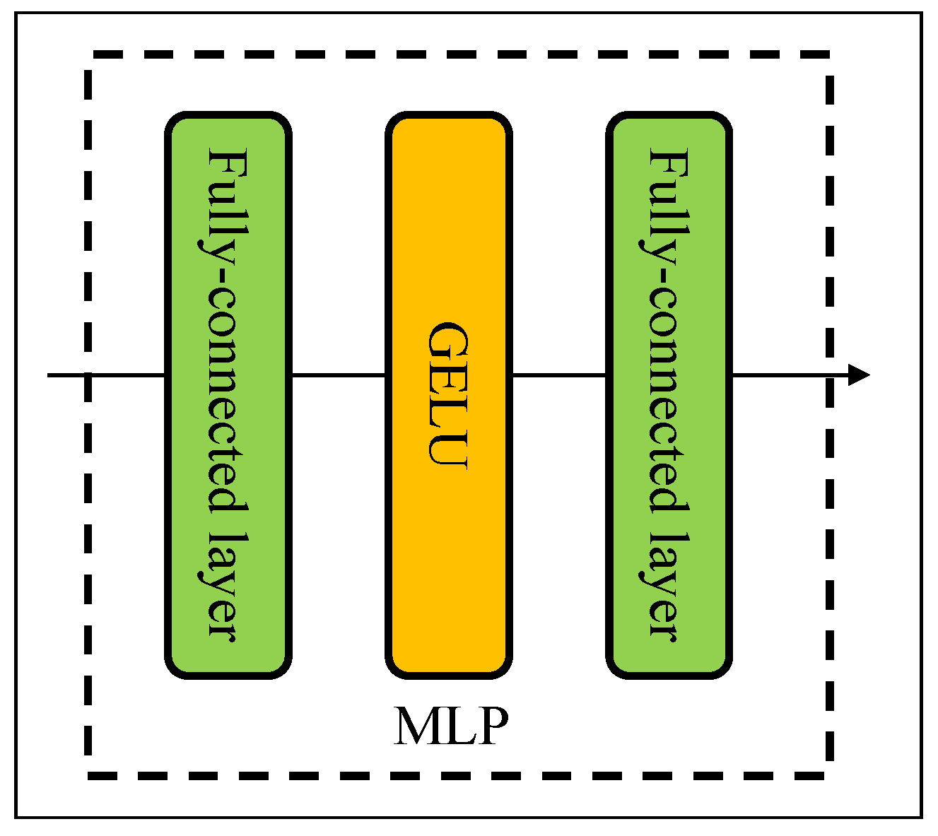
The structure of MLP is shown in Figure 3. In our study, a MLP consists of two fully connected layers and an element-wise nonlinearity of the nonlinearity activation function (GELU) [31]. The input of a mixer block comes from the pre-patch fully connected layer. Let X be the input feature map matrix, , where the features map has resolution and C is the number of feature maps or channels. The output of the token-mixing block (T) can be defined as follows:
where is the transpose operation, denotes the convolution operation on the transposed channel axis, and denotes GELU.
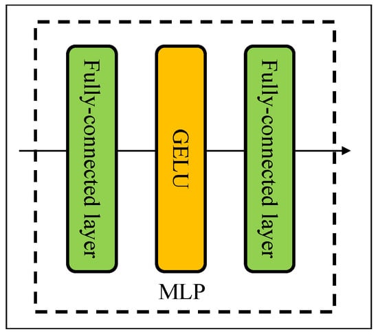
Figure 3.
The structure for MLP.
The introduction of an activation function increases the nonlinearity of the neural network model. At the same time, in order to improve the generalization ability of the neural network, it is necessary to add random regularization. In our study, we introduce a novel activation function—GELU. GELU is a synthesis of dropout, zoneout, and RELUs. It introduces the idea of random regularity in activation. It is a probabilistic description of neuron input, which is more intuitive and natural. GELU can be defined as follows:
where x is the input feature map and X is a Gaussian random variable with zero mean and unit variance. is the probability that X is less than or equal to a given value x. is the probability function of positive distribution. In our study, , and we approximate the GELU with
where is a hyperbolic tangent function.
At the end of the token-mixing block, we use the method to fuse the input feature maps and channel feature maps. The method is defined as follows:
where c is the channel number, ∗ is the convolution operation, is the kernel, and is the j-th Gaussian random variable with zero mean and unit variance. The method is a simple pixel overlay, which increases the amount of information describing the features of an image and maintains the consistency of the number of channels of the input and output feature map.
The channel-mixing block follows the token-mixing block, which is used to make contextual semantic fusion and control dimensions. The output of the semantic-mixing block can be defined as follows:
where is a kernel, is Batch Normalization layer, and is a data fusion method.
At the end of the semantic-mixing block, we use the method to fuse the output/input of HCSM and the output up-sampling layer of the backbone network.
where denotes the output of the channel-mixing block, denotes the input of the token-mixing block, and is the output of a mixing block. The is used to fuse feature maps from different channels, which can realize feature reuse. It should be noted that the dimensions of 3 feature maps must be consistent before using the method.
After the channel-mixing block, we obtain a mix feature with dimensions (bs; 1024; 1024). To prevent overfitting problems, we add a dropout layer (dropout = 0:5) before the final fully connected layer. Finally, the sigmoid activation function is added to predict the type of pest.
2.3. Evaluation Metrics
To verify the proposed model, the accuracy (Acc), precision (Prec), recall (Rec), and F1-score are used as metrics to evaluate the performance of all the comparative experiments:
where TP denotes the number of true positives, FP the number of false positives, TN the number of true negatives, and FN the number of false negatives.
3. Results
3.1. Experimental Settings
To evaluate the performance of PMLPNet, we validated our model on a dataset of 40 pest types. Our experimental setup is as follows: The model was constructed on the Tensorflow framework [32]. The main software and hardware of the computer and network configurations are shown in Table 2. All methods are trained/tested on a GeForce RTX 3090 GPU by NVIDIA in the United States. The model initialization parameters are set as follows: Learning rate is set to 0.001, epoch is set to 120, batch size is set to 8, the optimization algorithm is Adam, and loss function is binary cross entropy (BCE). In addition, we used the ReduceLROnPlateau and early stopping functions to reduce the learning rate and prevent overfitting problems. To ensure fairness in the comparison, we retained the structure and parameters of all comparison methods.
Table 2.
Computer and network configuration.
We split the samples into training, validation, and testing sets. The training and validation sets were used to train and fine-tune the comparison methods. The samples in the testing set were used to assess the proposed method against several comparison methods. The testing process was based on the best weight on the validation set. In the data preprocessing stage, we used the matrix complement or clipping method to unify all image sizes to pixels. The images and classification labels are input into the model after being converted into binary data. We divide 70% of the dataset into training sets, 20% into validation sets, and 10% into testing sets.
3.2. Comparison with State-of-the-Art Methods
We compared PMLPNet with several state-of-the-art deep learning methods, including VGG [33], GoogleNet [34], ResNet [35], DenseNet [36], CTransNet [37], ViT [38], BiT [39], and HaloNet [40]. All comparative methods come from publicly available code by these authors. Furthermore, we also compared the performance of these methods after pre-training on the ImageNet dataset. The experimental results are shown in Table 3.
Table 3.
Comparison of the state-of-the-art methods (”*-TL” denotes transfer learning method. ”*” stands for all).
As shown in Table 3, these 12 methods were divided into 2 groups: non-transfer learning-based methods (VGG-16, GoogleNet-TL, ResNet, DenseNet, CTransNet, BiT, ViT, HaloNet, and PMLPNet) and transfer learning-based methods (VGG-16-TL, ResNet50-TL, GoogleNet-TL, DenseNet50-TL, and Densenet201-TL). Among non-transfer learning-based methods, it is noted that the performance of models is proportional to their depth, such as VGG16 vs. GoogleNet vs. ResNet vs. DenseNet vs. CTransNet vs. BiT vs. ViT vs. HaloNet vs. PMLPNet (55.14% vs. 60.48% vs. 72.45% vs. 79.09% vs. 89.38% vs. 89.88% vs. 90.92% vs. 90.89% vs. 92.73%). Among all comparative methods, the performance of transfer learning-based methods exceeds that of non-transfer learning-based methods. This is mainly due to the fact that the pest images and the images in the ImageNet dataset are both natural images with similarity. Therefore, pre-training weights in the ImageNet dataset improves the performance of the classification models. Compared with other methods, our proposed method, PMLPNet, achieved the best classification results (accuracy: 92.73%, precision: 92.08%, recall: 93.10%, F1-score: 93.08%, and AUC: 0.88), which was mainly due to the fact that we use channel and spatial feature fusion to maximize the efficiency of feature extraction from patch images. PMLPNet integrates spatial contextual semantic features (i.e., the global capacity) and channel contextual semantic features (i.e., a local prior). This results in high-quality pixel positioning features for the fully connected layers and activation function, which helps the model to accurately classify pests.
3.3. Classification Performance of PMLPNet
In order to further analyze the performance of PMLPNet, in Figure 4, we used the confusion matrix thermodynamic diagram to show the results of the classification of 40 types of pests in the PMLPNet model. The numbers in the row and vertical coordinates represent 40 types of pests. The confusion matrix thermodynamic diagrams can display the prediction results of the summary classification model and summarize the situation analysis table of the records in the dataset in the form of a matrix according to the two criteria of real classification. Finally, the classification judgment is made by the classification model. The darker the color in the confusion matrix thermodynamic diagram, the larger the value. The larger the color difference of the color blocks in each line, the more unstable the prediction of the model. As shown in Figure 4, the diagonal color is relatively heavy, indicating that PMLPNet can distinguish most pests. However, the recognition accuracy of PMLPNet on each type of pest varies greatly. Firstly, the color depth of the squares on the diagonal is different, which means that there is a difference in the recognition accuracy of PMLPNet for pests. In addition, the color depth of each line in the confusion matrix thermogram is different, which means that PMLPNet predicts the species of pests incorrectly. The color difference of some squares in the line is very large, especially for the type with a relatively light color in the diagonal area. For example, the blocks on the diagonal corresponding to the 3 (Callitettix versicolor (Fabricius)) and 23 (Laodelphax striatellus (Fallen)) pests are lighter than the other diagonal colors. This indicates that the classification difficulty of these two pests is greater than that of other pests.
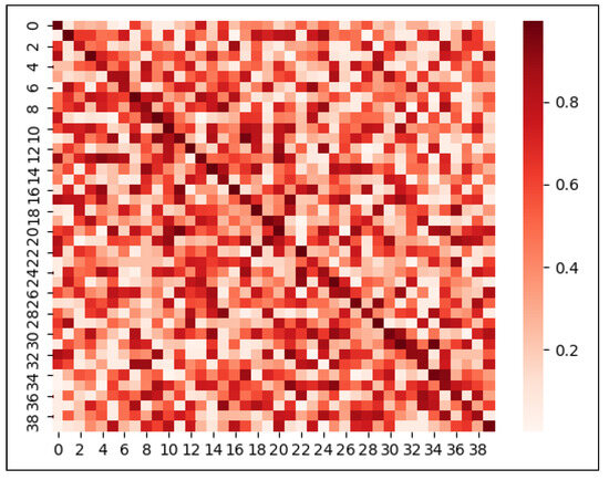
Figure 4.
Confusion matrix thermodynamic image of 40 types of pests on PMLPNet.
3.4. Visualization Analysis
In addition, we used the GradCAM method to display thermodynamic diagrams of eight typical pest images. All GradCAM visualizations come from the last convolutional layer of PMLPNet. The visualization results are shown in Figure 5. The images in rows (a) and (c) of Figure 5 show the original images, and the images in rows (b) and (c) represent the GradCAM thermodynamic diagrams that correspond to the images in rows (a) and (c). The highlighted part of the GradCAM thermodynamic diagrams shows the area of interest for our model. The thermal images in row (b) show that the area of interest exactly covers the location of the pest, which means that our model can extract features from key areas; this is very beneficial for the model’s ability to complete predictions correctly. The experimental results show that the classification accuracy of the PMLPNet model for the four images in row (a) exceeds 99.73%, 98.96%, 99.04%, and 99.31%, respectively. It should be noted that the four images in row (a) have a single background, prominent pest targets, and sufficient lighting, which is also the reason why the model can classify these correctly. The pests in the first picture even overlap and the fourth picture contains a large gap within the same type of pest. However, the original images in row (c) have complex backgrounds, insufficient lighting, and scattered and blurry targets, which makes it difficult to fully cover the thermal map area in row (d) and the pest area in the original image. Due to the above reasons, the performance of PMLPNet in extracting features from these four types of images and performing classification predictions has been affected (with accuracy rates of 76.45%, 56.34%, 72.08%, and 70.00%, respectively). For example, due to the similarity between the pest and the background colors in the first and second images of row (c), it is difficult for the model to accurately extract the features of the pests’ location. However, due to lighting issues in the fourth image, our model focuses more on the highlighted areas and ignores other parts of the pest.
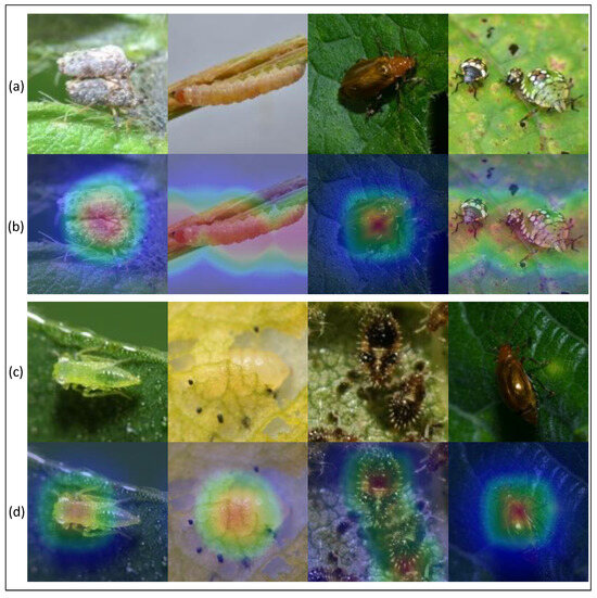
Figure 5.
Qualitative results. (a,c) are original images, and (b,d) are visualized thermal maps.
3.5. Ablation Experiment
We conducted an ablation study to provide in-depth insights into the effectiveness of the different components in PMLPNet on multi-class pest classification. We analyzed the effectiveness of the components separately for pest classification. In Table 4, we extended four ablation experiments: (1) verifying the influence of transfer learning on model performance; (2) verifying the influence of image and patch strategy on model performance; (3) verifying the influence of transpose operation on model performance; (4) verifying the influence of the number of mixer block on model performance.
Table 4.
The impacts of structure on PMLPNet; “no T” denotes no transpose operation in the PMLPNet and “*-TL” denotes transfer learning method. “*” stands for all.
As shown in Table 4, the performance of the MLP-based PMLPNet model is much higher than that of methods without MLP. Due to the removal of the MLP module in PMLPNet (no T), the two models degenerated into models similar to VGG. Although both models included a strategy for feature map transposition, it had little impact on the performance of the model. The introduction of transfer learning has greatly improved the performance of PMLPNet (no T), which means that the transfer learning strategy based on the ImageNet dataset is effective in pest image classification. In addition, under the same conditions, the performance of patch-based methods is higher than that of image-based methods. For example, the accuracy of patch-based PMLPNet (no T) improved by 7.81%, patch-based PMLPNet-TL improved by 3.69%, and patch-based PMLPNet improved by 6.39%, respectively. This is mainly due to the fact that patch-based PMLPNet can obtain global features from patches through a fully connected layer and MLP, which is beneficial for detecting small-sized pests. Image-based methods may lead to the loss of long-distance features, which is harmful for the detection of small-sized pests. Furthermore, to verify the influence of different numbers of mixer blocks on model performance, we embedded four, eight, and ten mixer blocks in patch lever-based PMLPNet, respectively. This choice was based on the research experience of Google [30]. The results are shown in Table 4, with PMLPNet performing best at eight mixer blocks. Finally, we ended up embedding eight mixer blocks in PMLPNet.
In addition, we also evaluated the effect of activation functions on model performance, including ReLU, Leaky ReLU, ELU, PReLU, and GELU. An activation function is a function added to an artificial neural network to help the network learn complex patterns in data. The experimental results are shown in Table 5. All five activation functions help the model obtain better performance, among which PMLPNet using GELU as the activation function achieves the best performance. Finally, we chose GELU as the activation function of the proposed model.
Table 5.
The impacts of activation function on PMLPNet.
3.6. Generalization Performance of PMLPNet
To verify the generalization of CTransNet, we conducted extended experiments on another two pest image datasets.
- (1)
- IP102 [41]. This is a crop pest and disease dataset for target classification and detection tasks, which contains more than 75,000 images of 8 crops: rice, corn, wheat, sugar beet, alfalfa, grape, citrus, and mango. In our experiment, we downloaded 8000 images involving 8 crops, with 1000 images for each crop. In our experiment with additional validation, we aim to verify the ability of the proposed model to distinguish leaf types from images.
- (2)
- PlantDoc [42]. This is a publicly available dataset published by the Indian Institute of Technology, includes 2598 leaf images involving 13 types of plants, and covers a wide variety of crops commonly found in agriculture. These images not only included healthy leaves but also focused on the performance of different diseases on leaves, covering 27 categories (17 diseases; 10 healthy). This dataset is used for image classification and object detection. In our study, our main goal was to verify the classification performance of the proposed model, so we only verified the classification performance of the model for leaf types on this dataset.
We verified the generalization performance of PMLPNet on these two additional datasets using the optimized network parameters of the collected datasets. The verification results are shown in Table 6. The evaluation indexes are from Wu et al. [41] and Singh et al. [42], respectively. We revalidated the performance of these methods on the IP102 dataset. In addition, we verified the performance of these methods on the PlantDoc dataset, except for VGG-16-TL and GoogleNet-TL, two experimental results from Singh et al. [42]. As shown in Table 6, our proposed model achieved the best performance on both datasets (accuracy of 68.32% and 76.52%, respectively). Because the leaves of both datasets contain various diseases, the leaves have complex texture and pixel relationships, which affects the classification performance of PMLPNet. In addition, the pre-training weights of the additional validation experiments are based on PMLPNet, and the differences between the original dataset and the additional dataset will also affect the performance of the proposed model. The methods in Wu et al. [41] and Singh et al. [42] were proposed in 2019 and 2020, respectively, and our proposed model has more advantages. Overall, the classification performance of PMLPNet is very good, and the generalization performance is also very strong.
Table 6.
Comparison results on IP102 and PlantDoc datasets.
4. Discussion
We propose a patch-based multi-layer perceptron neural network (PMLPNet) for multi-class pest classification. PMLPNet integrates spatial contextual semantic features and channel contextual semantic features. This results in high-quality pixel positioning features for the fully connected layers and activation function, which helps the model to accurately classify pests. Finally, we validated our proposed model on a multi-class pest dataset and compared it with other advanced models. PMLPNet achieved state-of-the-art performance. In addition, we visualized the heterogeneity of the extracted features and patches, verified the performance of the model, and analyzed the impact of image quality on model performance.
In this study, we extracted features from patch-level images and completed the prediction of pest species on image level. The background and foreground of patches from the same image are different, so the feature information obtained by the model from each patch is also different. Therefore, we believe that there are differences in the degree of closeness between these patches and pest species. Taking aphid images as an example, we selected nine patches based on this image for probability analysis of pest species prediction to verify the heterogeneity between patches in the same image.
As shown in Figure 6, we input an aphid image into the PMLPNet model. After PMLPNet extracts the features, we display the prediction probability of each patch on the original image. The left side of Figure 6 shows the input image, and the right side shows the details of the predicted probability for each patch. For an aphid image, the prediction probabilities of different patches vary greatly. This means that this probability difference can also lead to differences in feature extraction. Our proposed model can distinguish between the target area and background, but for patches that also contain the target, there is a difference in the prediction probability of our model (0.94 vs. 0.83 vs. 0.75), mainly due to the size of the difference between the pixels corresponding to aphids and the surrounding background pixels. When there is a significant difference between aphids and the surrounding background, the model can accurately determine that the target identified in the patch is aphids (0.94). However, when the pixels corresponding to aphids in the image overlap or are similar to the background pixels, the model’s recognition accuracy for aphids will be reduced. In addition, if the pixels corresponding to aphids have a small proportion of space and there are similar pixels, the recognition accuracy of the model will be greatly reduced (0.75). Based on the above reasons, the complexity of the image background and the size of the pests are factors that affect the performance of the model in classifying pests.
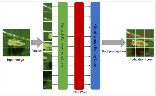
Figure 6.
Intra-image heterogeneity by patch predictions. The left image is the original input image. The right image shows the detail of the predicted probability of each patch.
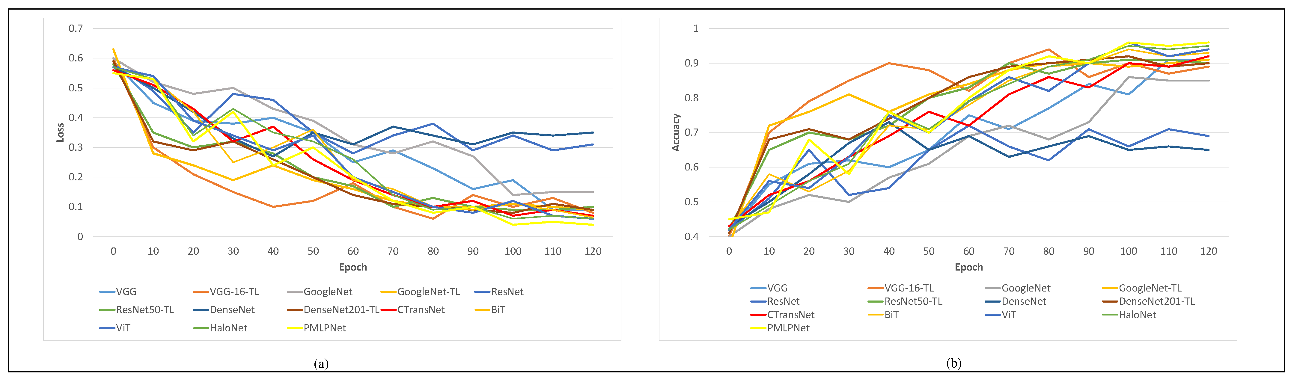
As shown in Figure 7, we conducted statistical analysis on the loss and accuracy of nine comparison methods during the training process, and generated curves. We set the epoch of all comparison methods to 120; as the epoch increases, the loss values of all models decrease while the accuracy improves. As shown in Figure 7a, when the epoch value is 100, most models have the lowest losses, except for VGG and ResNet. As shown in Figure 7b, most models also achieved the highest accuracy, except for VGG, ResNet, and DenseNet. Based on Figure 7a,b, it can be concluded that most models obtain their optimal state when epoch = 100. When epoch is greater than 100, it increases the likelihood of overfitting problems.
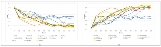
Figure 7.
Loss and accuracy curves of comparative methods. (a) is the loss cureves of comparative methods, (b) is the accuracy curves of comparative methods.
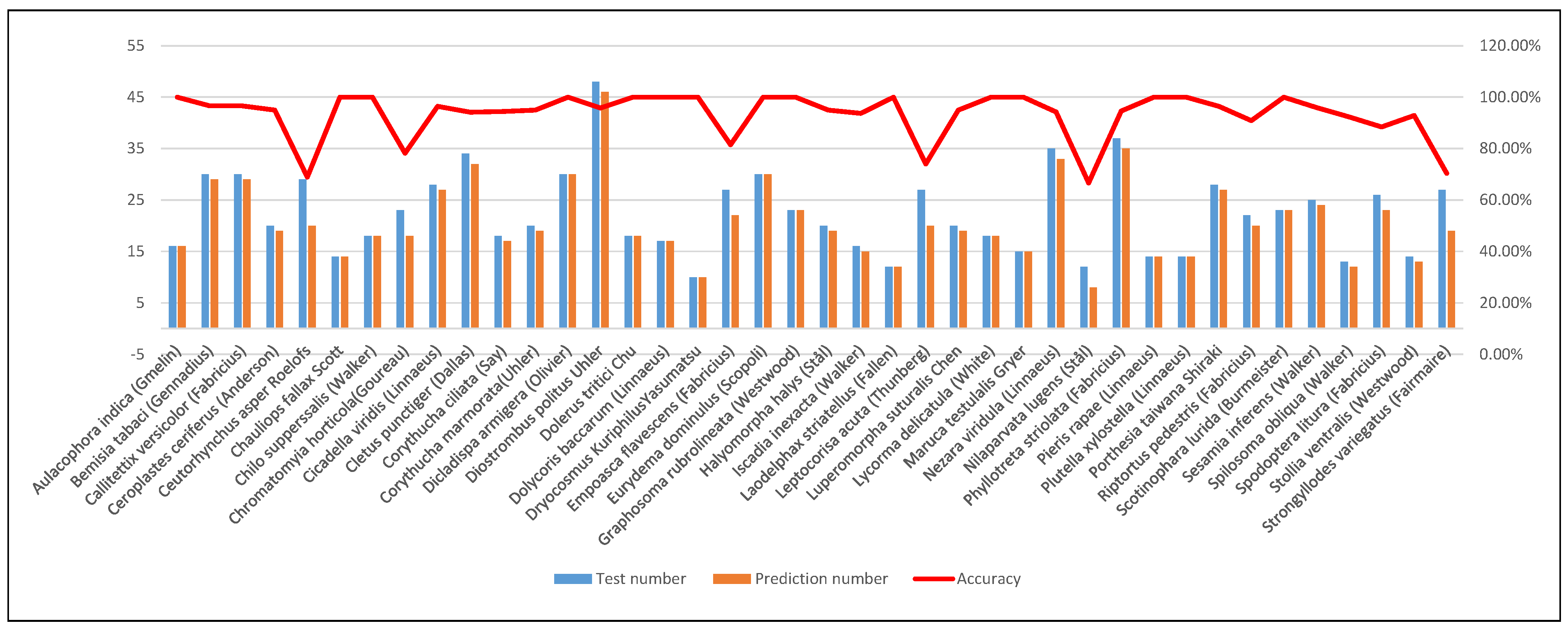
In addition, we conducted statistical analysis on the accuracy of the proposed PMLPNet in predicting 40 types of pests in the testing set. Specifically, we calculate the number of each type of pest in the testing set and the correct number predicted by the model, and calculate the accuracy of this type of pest prediction (as shown in Figure 8). Figure 8 is a combination figure, including a histogram chart and a line chart. The histogram chart shows the number of each type of pest and the number of correctly predicted pests in the testing set, and the line chart shows the prediction accuracy of the testing set. As shown by the red line in Figure 8, the prediction accuracy of most pests exceeds 90%, and some even reach 100%. Through image analysis, we found that these pests have a large size in the image and have significant differences in color and background. There are also obvious turning points on the red line, which correspond to lower accuracy. This means that our proposed model has a higher error rate in identifying such pests. We analyzed and found that the main reasons for this situation are the following three aspects: (1) The small size of pests in the images, such as and å; (2) The background of the image where the pest is located is complex, such as and ; (3) The image lacks sufficient lighting, such as . The above issues have affected the performance of our model, which demonstrates its limitations. We will focus on these issues in our future research.
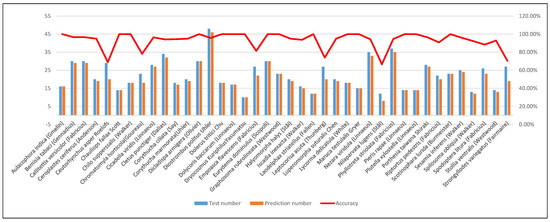
Figure 8.
Combination figure of predictive analysis for each class of pests on PMLPNet.
Our research has some limitations. Firstly, there is a contradiction between the limited sample size and the training sample requirements of deep learning models. Although data augmentation can alleviate the contradiction between the two, collecting more samples is the ultimate solution. In addition, mixer block is a time-consuming module, and the training time of this model is relatively long. Secondly, the heterogeneity between the source and target data in transfer learning limits the performance of transfer learning methods. Finally, the classification accuracy of complex backgrounds, insufficient lighting, and scattered and blurry targets still needs to be improved.
5. Conclusions
In this study, our proposed PMLPNet has been proven to effectively identify different types of pests. This model has achieved excellent performance in automatic classification of multiple types of pests, with an accuracy rate of 92.73%. The successful application of this technology will help agricultural researchers and farmers detect and diagnose pest types, which is of great significance for the prevention and treatment of crop pests. This method is expected to be more widely applied in agriculture. In addition, this study further investigated the differences in different types of pests and the heterogeneity in images, providing new ideas for pest classification research. More importantly, the additional experiments on IP102 and PlantDoc prove PMLPNet has good generalization performance. In future work, we plan to further improve the network architecture to address current limitations.
Author Contributions
L.L. and H.Q.: Conceptualization, methodology, software, visualization, writing original draft. J.C.: Collecting data and conducting experiments. J.X. and S.Q.: Analyzing experimental results. X.X.: conducted additional experiments. All authors have read and agreed to the published version of the manuscript.
Funding
This work was funded by the National Key R&D Program of China (3502300), the Henan Provincial Key Research and Promotion Projects (No. 242102211012), the National Key R&D projects during the 14th Five Year Plan period of China (No. 2022YFD1400302), and the National Natural Science Foundation of China (Grant No. 82274370).
Data Availability Statement
The data presented in this study are available on request from the corresponding author due to the research project is still ongoing, the dataset is not available for the time being.
Conflicts of Interest
The authors declare that they have no known competing financial interests or personal relationships that could have appeared to influence the work reported in this paper.
References
- Estruch, J.J.; Carozzi, N.B.; Desai, N.; Duck, N.B.; Warren, G.W.; Koziel, M.G. Transgenic plants: An emerging approach to pest control. Nat. Biotechnol. 1997, 15, 137–141. [Google Scholar] [CrossRef]
- Li, Z.; Paul, R.; Ba Tis, T.; Saville, A.C.; Hansel, J.C.; Yu, T.; Ristaino, J.B.; Wei, Q. Non-invasive plant disease diagnostics enabled by smartphone-based fingerprinting of leaf volatiles. Nat. Plants 2019, 5, 856–866. [Google Scholar] [CrossRef] [PubMed]
- Alves, A.N.; Souza, W.S.; Borges, D.L. Cotton pests classification in field-based images using deep residual networks. Comput. Electron. Agric. 2020, 174, 105488. [Google Scholar] [CrossRef]
- Wang, F.; Wang, R.; Xie, C.; Zhang, J.; Li, R.; Liu, L. Convolutional neural network based automatic pest monitoring system using hand-held mobile image analysis towards non-site-specific wild environment. Comput. Electron. Agric. 2021, 187, 106268. [Google Scholar] [CrossRef]
- Guo, X.; Zhou, H.; Su, J.; Hao, X.; Tang, Z.; Diao, L.; Li, L. Chinese agricultural diseases and pests named entity recognition with multi-scale local context features and self-attention mechanism. Comput. Electron. Agric. 2020, 179, 105830. [Google Scholar] [CrossRef]
- Zou, Z.; Chen, K.; Shi, Z.; Guo, Y.; Ye, J. Object detection in 20 years: A survey. Proc. IEEE 2023, 111, 257–276. [Google Scholar] [CrossRef]
- Liu, L.; Ying, Y.; Fei, Z.; Min, L.; Wang, J. An interpretable boosting model to predict side effects of analgesics for osteoarthritis. BMC Syst. Biol. 2018, 12, 105. [Google Scholar] [CrossRef]
- Liu, L.; Tang, S.; Wu, F.; Wang, Y.P.; Wang, J. An ensemble hybrid feature selection method for neuropsychiatric disorder classification. IEEE/ACM Trans. Comput. Biol. Bioinform. 2021, 19, 1459–1471. [Google Scholar] [CrossRef]
- Liu, L.; Wang, Y.; Chang, J.; Zhang, P.; Xiong, S.; Liu, H. A correlation graph attention network for classifying chromosomal instabilities from histopathology whole-slide images. iScience 2023, 26, 106874. [Google Scholar] [CrossRef]
- LeCun, Y.; Bengio, Y.; Hinton, G. Deep learning. Nature 2015, 521, 436–444. [Google Scholar] [CrossRef]
- Liu, L.; Cheng, J.; Quan, Q.; Wu, F.X.; Wang, Y.P.; Wang, J. A survey on U-shaped networks in medical image segmentations. Neurocomputing 2020, 409, 244–258. [Google Scholar] [CrossRef]
- Hassan, S.M.; Maji, A.K.; Jasiński, M.; Leonowicz, Z.; Jasińska, E. Identification of plant-leaf diseases using CNN and transfer-learning approach. Electronics 2021, 10, 1388. [Google Scholar] [CrossRef]
- Naik, B.N.; Malmathanraj, R.; Palanisamy, P. Detection and classification of chilli leaf disease using a squeeze-and-excitation-based CNN model. Ecol. Inform. 2022, 69, 101663. [Google Scholar] [CrossRef]
- Bari, B.S.; Islam, M.N.; Rashid, M.; Hasan, M.J.; Razman, M.A.M.; Musa, R.M.; Ab Nasir, A.F.; Majeed, A.P.A. A real-time approach of diagnosing rice leaf disease using deep learning-based faster R-CNN framework. PeerJ Comput. Sci. 2021, 7, e432. [Google Scholar] [CrossRef] [PubMed]
- Gautam, V.; Trivedi, N.K.; Singh, A.; Mohamed, H.G.; Noya, I.D.; Kaur, P.; Goyal, N. A transfer learning-based artificial intelligence model for leaf disease assessment. Sustainability 2022, 14, 13610. [Google Scholar] [CrossRef]
- Al-gaashani, M.S.; Shang, F.; Muthanna, M.S.; Khayyat, M.; Abd El-Latif, A.A. Tomato leaf disease classification by exploiting transfer learning and feature concatenation. IET Image Process. 2022, 16, 913–925. [Google Scholar] [CrossRef]
- Paymode, A.S.; Malode, V.B. Transfer learning for multi-crop leaf disease image classification using convolutional neural network VGG. Artif. Intell. Agric. 2022, 6, 23–33. [Google Scholar] [CrossRef]
- Thangaraj, R.; Anandamurugan, S.; Kaliappan, V.K. Automated tomato leaf disease classification using transfer learning-based deep convolution neural network. J. Plant Dis. Protect. 2021, 128, 73–86. [Google Scholar] [CrossRef]
- Krishnamoorthy, N.; Prasad, L.N.; Kumar, C.P.; Subedi, B.; Abraha, H.B.; Sathishkumar, V. Rice leaf diseases prediction using deep neural networks with transfer learning. Environ. Res. 2021, 198, 111275. [Google Scholar]
- Pallathadka, H.; Ravipati, P.; Sajja, G.S.; Phasinam, K.; Kassanuk, T.; Sanchez, D.T.; Prabhu, P. Application of machine learning techniques in rice leaf disease detection. Mater. Today Proc. 2022, 51, 2277–2280. [Google Scholar] [CrossRef]
- Liu, Z.; Gao, J.; Yang, G.; Zhang, H.; He, Y. Localization and classification of paddy field pests using a saliency map and deep convolutional neural network. Sci. Rep. 2016, 6, 20410. [Google Scholar] [CrossRef]
- Xie, C.; Wang, R.; Zhang, J.; Chen, P.; Dong, W.; Li, R.; Chen, T.; Chen, H. Multi-level learning features for automatic classification of field crop pests. Comput. Electron. Agric. 2018, 152, 233–241. [Google Scholar] [CrossRef]
- Too, E.C.; Yujian, L.; Njuki, S.; Yingchun, L. A comparative study of fine-tuning deep learning models for plant disease identification. Comput. Electron. Agric. 2019, 161, 272–279. [Google Scholar] [CrossRef]
- Gu, Y.; Piao, Z.; Yoo, S.J. STHarDNet: Swin transformer with HarDNet for MRI segmentation. Appl. Sci. 2022, 12, 468. [Google Scholar] [CrossRef]
- Cheng, J.; Liu, J.; Kuang, H.; Wang, J. A fully automated multimodal MRI-based multi-task learning for glioma segmentation and IDH genotyping. IEEE Trans. Med. Imaging 2022, 41, 1520–1532. [Google Scholar] [CrossRef] [PubMed]
- Pereira, S.; Pinto, A.; Amorim, J.; Ribeiro, A.; Alves, V.; Silva, C.A. Adaptive feature recombination and recalibration for semantic segmentation with fully convolutional networks. IEEE Trans. Med. Imaging 2019, 38, 2914–2925. [Google Scholar] [CrossRef] [PubMed]
- Saranya, T.; Deisy, C.; Sridevi, S. Efficient agricultural pest classification using vision transformer with hybrid pooled multihead attention. Comput. Biol. Med. 2024, 177, 108584. [Google Scholar] [CrossRef] [PubMed]
- Kamilaris, A.; Prenafeta-Boldú, F.X. Deep learning in agriculture: A survey. Comput. Electron. Agric. 2018, 147, 70–90. [Google Scholar] [CrossRef]
- Sladojevic, S.; Arsenovic, M.; Anderla, A.; Culibrk, D.; Stefanovic, D. Deep neural networks based recognition of plant diseases by leaf image classification. Comput. Intell. Neurosci. 2016, 2016, 3289801. [Google Scholar] [CrossRef]
- Tolstikhin, I.O.; Houlsby, N.; Kolesnikov, A.; Beyer, L.; Zhai, X.; Unterthiner, T.; Yung, J.; Steiner, A.; Keysers, D.; Uszkoreit, J.; et al. Mlp-mixer: An all-mlp architecture for vision. Adv. Neural Inf. Process. Syst. 2021, 34, 24261–24272. [Google Scholar]
- Hendrycks, D.; Gimpel, K. Gaussian error linear units (gelus). arXiv 2016, arXiv:1606.08415. [Google Scholar]
- Abadi, M.; Barham, P.; Chen, J.; Chen, Z.; Davis, A.; Dean, J.; Devin, M.; Ghemawat, S.; Irving, G.; Isard, M.; et al. Tensorflow: A system for large-scale machine learning. In Proceedings of the 12th USENIX Symposium on Operating Systems Design and Implementation (OSDI 16), Savannah, GA, USA, 2–4 November 2016; pp. 265–283. [Google Scholar]
- Simonyan, K.; Zisserman, A. Very deep convolutional networks for large-scale image recognition. arXiv 2014, arXiv:1409.1556. [Google Scholar]
- Szegedy, C.; Liu, W.; Jia, Y.; Sermanet, P.; Reed, S.; Anguelov, D.; Erhan, D.; Vanhoucke, V.; Rabinovich, A. Going deeper with convolutions. In Proceedings of the IEEE Conference on Computer Vision and Pattern Recognition, Boston, MA, USA, 7–12 June 2015; pp. 1–9. [Google Scholar]
- He, K.; Zhang, X.; Ren, S.; Sun, J. Deep residual learning for image recognition. In Proceedings of the IEEE Conference on Computer Vision and Pattern Recognition, Las Vegas, NV, USA, 27–30 June 2016; pp. 770–778. [Google Scholar]
- Huang, G.; Liu, Z.; Van Der Maaten, L.; Weinberger, K.Q. Densely connected convolutional networks. In Proceedings of the IEEE Conference on Computer Vision and Pattern Recognition, Honolulu, HI, USA, 21–26 July 2017; pp. 4700–4708. [Google Scholar]
- Liu, L.; Wang, Y.; Zhang, P.; Qiao, H.; Sun, T.; Zhang, H.; Xu, X.; Shang, H. Collaborative Transfer Network for Multi-Classification of Breast Cancer Histopathological Images. IEEE J. Biomed. Health Inform. 2024, 28, 110–121. [Google Scholar] [CrossRef] [PubMed]
- Dosovitskiy, A.; Beyer, L.; Kolesnikov, A.; Weissenborn, D.; Houlsby, N. An Image is Worth 16x16 Words: Transformers for Image Recognition at Scale. arXiv 2020, arXiv:2010.11929. [Google Scholar]
- Kolesnikov, A.; Beyer, L.; Zhai, X.; Puigcerver, J.; Yung, J.; Gelly, S.; Houlsby, N. Big transfer (bit): General visual representation learning. In Proceedings of the Computer Vision–ECCV 2020: 16th European Conference, Glasgow, UK, 23–28 August 2020; Proceedings, Part V 16. Springer: Berlin, Germany, 2020; pp. 491–507. [Google Scholar]
- Vaswani, A.; Ramachandran, P.; Srinivas, A.; Parmar, N.; Hechtman, B.; Shlens, J. Scaling local self-attention for parameter efficient visual backbones. In Proceedings of the IEEE/CVF Conference on Computer Vision and Pattern Recognition, Nashville, TN, USA, 20–25 June 2021; pp. 12894–12904. [Google Scholar]
- Wu, X.; Zhan, C.; Lai, Y.K.; Cheng, M.M.; Yang, J. IP102: A Large-Scale Benchmark Dataset for Insect Pest Recognition. In Proceedings of the 2019 IEEE/CVF Conference on Computer Vision and Pattern Recognition (CVPR), Long Beach, CA, USA, 15–20 June 2019. [Google Scholar]
- Singh, D.; Jain, N.; Jain, P.; Kayal, P.; Batra, N. PlantDoc: A Dataset for Visual Plant Disease Detection. In Proceedings of the CoDS COMAD 2020: 7th ACM IKDD CoDS and 25th COMAD, Hyderabad, India, 5–7 January 2020. [Google Scholar]


Disclaimer/Publisher’s Note: The statements, opinions and data contained in all publications are solely those of the individual author(s) and contributor(s) and not of MDPI and/or the editor(s). MDPI and/or the editor(s) disclaim responsibility for any injury to people or property resulting from any ideas, methods, instructions or products referred to in the content. |
© 2024 by the authors. Licensee MDPI, Basel, Switzerland. This article is an open access article distributed under the terms and conditions of the Creative Commons Attribution (CC BY) license (https://creativecommons.org/licenses/by/4.0/).