Optimization of Support Vector Machine with Biological Heuristic Algorithms for Estimation of Daily Reference Evapotranspiration Using Limited Meteorological Data in China

Abstract

Precise estimation of daily reference crop evapotranspiration (ET₀) is critical for water resource management and agricultural irrigation optimization worldwide. In China, diverse climatic zones pose challenges for accurate ET₀ prediction. Here, we evaluate the performance of a support vector machine (SVM) and its hybrid models, PSO-SVM and WOA-SVM, utilizing meteorological data spanning 1960–2020. Our study aims to identify a high-precision, low-input ET₀ estimation tool. The findings indicate that the hybrid models, particularly WOA-SVM, demonstrated superior accuracy with R² values ranging from 0.973 to 0.999 and RMSE values between 0.123 and 0.863 mm/d, outperforming the standalone SVM model with R² values of 0.955 to 0.989 and RMSE values of 0.168 to 0.982 mm/d. The standalone SVM model showed relatively lower accuracy with R² values of 0.822 to 0.887 and RMSE values of 0.381 to 1.951 mm/d. Notably, the WOA-SVM model, with R² values of 0.990 to 0.992 and RMSE values of 0.092 to 0.160 mm/d, emerged as the top performer, showcasing the benefits of the whale optimization algorithm in enhancing SVM’s predictive capabilities. The PSO-SVM model also presented improved performance, especially in the temperate continental zone (TCZ), subtropical monsoon region (SMZ), and temperate monsoon zone (TMZ), when using limited meteorological data as the input. The study concludes that the WOA-SVM model is a promising tool for high-precision daily ET₀ estimation with fewer meteorological parameters across the different climatic zones of China.

1. Introduction

Reference evapotranspiration (ET₀) is a critical parameter within the soil–plantsoil–atmosphere continuum (SPAC) [1]. Accurate estimation of ET₀ is essential for assessing crop water requirements and is a prerequisite for the optimal design of agricultural irrigation systems [2,3,4]. The ever-changing global climate presents challenges to agriculture, which in turn affects the soil–water balance and the magnitude of ET₀ [5,6,7]. The high-precision estimation of ET₀ is, therefore, crucial for addressing crop water demand and provides a valuable reference for the formulation of irrigation schedules [8,9].

Despite the global significance of reference crop evapotranspiration (ET₀) in agricultural and hydrological applications, direct observation of ET₀ remains elusive in many parts of the world [10,11]. Therefore, it is imperative to utilize empirical models with varying input factors to reasonably simulate ET₀. However, while empirical models, like the Priestley–Taylor and Hargreaves models, are convenient due to their minimal data demands, they are not without limitations. These models, typically tailored to specific regions, may not consistently offer accurate predictions across different climates, and their dependence on a limited set of meteorological parameters can be restrictive, especially in regions where comprehensive data are sparse [12,13]. The FAO-56 Penman–Monteith model, despite its superior accuracy and theoretical soundness, also faces practical implementation challenges due to the extensive climatic data it requires, which can be a barrier in areas lacking robust meteorological infrastructure [4,14]. The limitations of these empirical models highlight the critical need for the development of models that are more adaptive to local conditions and capable of providing reliable ET₀ estimations regardless of data availability [15].

The relationship between reference crop evapotranspiration (ET₀) and the factors influencing it is characterized by complex nonlinear dynamics, a challenge that empirical models often struggle to capture accurately [16]. Traditional empirical models, while straightforward, are limited in their ability to adapt to the intricate variations present in meteorological data across diverse climates. In contrast, machine learning models have shown great promise in dealing with such nonlinear complexities, offering a superior approach to modeling the nuanced interactions at play [17,18,19]. Among these, the extreme learning machine (ELM) [20], SVM [21], random forest (RF) [22], and artificial neural networks (ANNs) [23] stand out for their distinct advantages in handling large and complex datasets. ELM is recognized for its rapid training capabilities [24,25], RF for its robustness in managing numerous variables [26], ANNs for their adaptive learning [27], and SVM for its exceptional capacity to generalize from limited data, its effectiveness in high-dimensional spaces, and its resilience against overfitting [28]. Support vector machines offer robust generalization, excel with high-dimensional data, and exhibit strong robustness to outliers in regression problem-solving. These attributes render SVMs particularly adept in practical applications involving intricate data relationships. After a thorough evaluation of these models’ capabilities and their suitability for capturing the nonlinearity of ET₀ estimation, our study has chosen to employ an SVM.

While machine learning models like SVMs have demonstrated exceptional capabilities in addressing the nonlinear dynamics of estimating daily reference crop evapotranspiration (ET₀), their performance can be highly sensitive to the selection of hyperparameters. The task of tuning these parameters is non-trivial, as it often involves searching through a high-dimensional space where the optimal set can dramatically influence the model’s predictive accuracy. To overcome this challenge, various metaheuristic algorithms have been widely adopted to optimize hyperparameters effectively [29,30]. Algorithms such as PSO, the WOA, genetic algorithms (GAs), and simulated annealing (SA) are notable for their ability to navigate complex search spaces and converge towards optimal solutions. PSO and WOA, among other algorithms, have consistently demonstrated remarkable effectiveness across a spectrum of research. The necessity for parameter optimization in SVMs is met by the proven optimization capabilities of WOAs and PSOs, which have demonstrated their effectiveness in various studies. The particle swarm optimization algorithm, with its potent global search and ease of implementation, and the whale optimization algorithm, with its swift convergence inspired by whale foraging, are both highly effective. WOA, in particular, enhances global search by diversifying search locations, a strategy that has been widely adopted and praised in the literature. PSO, inspired by the social behavior of bird flocks, is particularly effective in exploring broad hyperparameter landscapes [31,32], while a WOA, which mimics the bubble-net hunting strategy of humpback whales, excels at fine-tuning and local search optimization [33]. Jia et al. [34] utilized the PSO algorithm to optimize the hyperparameters within the long short-term memory neural network for the prediction of daily ET₀. The study demonstrated that the optimized model exhibited commendable predictive accuracy in ET₀ forecasting. Wu et al. [35] evaluated the performance of 12 empirical models for predicting ET₀, which included four temperature-based models, five radiation-based models, and three hybrid models. They optimized the parameters of the optimal models using the WOA. The study results indicated that the models optimized by a WOA achieved higher accuracy and better generalization capabilities. By integrating these algorithms with machine learning models, researchers have developed hybrid models that leverage the strengths of both worlds: the predictive power of machine learning and the optimization prowess of metaheuristics. In our study, we have chosen to apply PSO and a WOA to fine-tune the hyperparameters of our SVM model, aiming to enhance its performance in ET₀ estimation by constructing a hybrid model that combines the best of both optimization and learning strategies.

As a robust machine learning model, the SVM has demonstrated its effectiveness in predicting reference crop evapotranspiration (ET₀). However, the optimization of its parameters remains a challenge that can affect the model’s performance, particularly when dealing with the complex nonlinear relationships inherent in meteorological data. To address this, the present study integrates biological heuristic algorithms with the SVM model to enhance its parameter optimization capabilities. The primary objectives of this research are as follows:

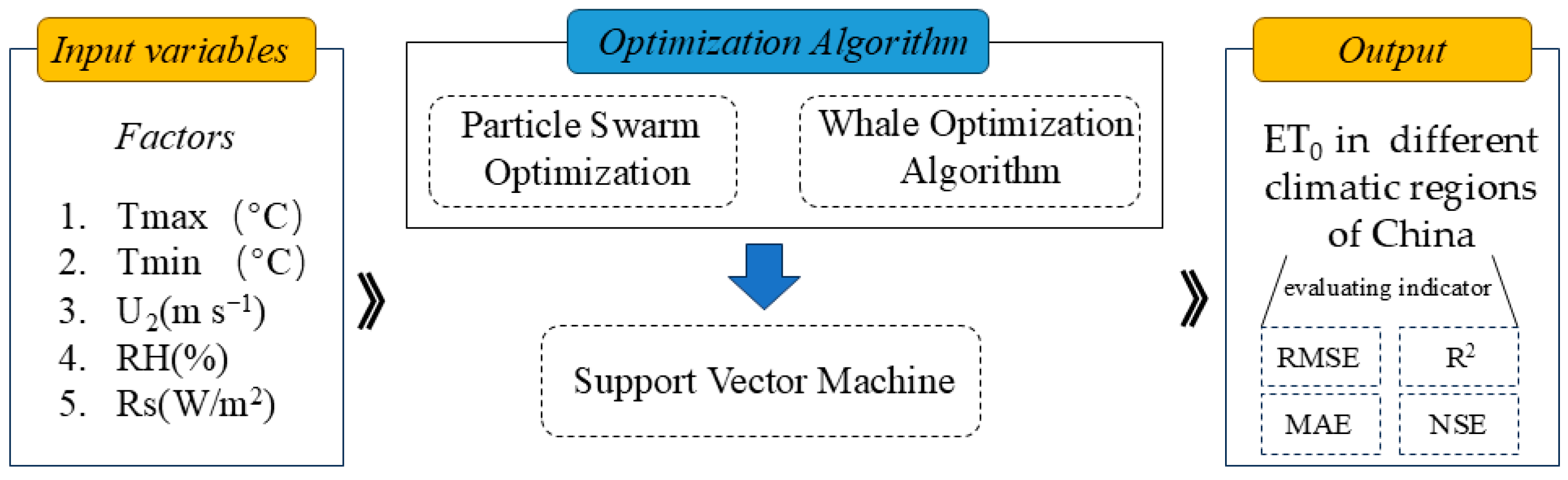
• To assess the efficacy of two biological heuristic algorithms—PSO and the WOA—in refining the SVM model for daily ET₀ estimation;
• To conduct a comparative analysis of the performance of the hybrid SVM models and the standalone SVM model under conditions with limited meteorological data, focusing on their accuracy in ET₀ estimation;
• To identify the adaptability of the estimation models, based on key input factors, to the different climatic zones of China.

2. Materials and Methods

2.1. Data Sources

The meteorological data used in the present study were obtained from the China Meteorological Data Network (http://data.cma.cn/, accessed on 10 June 2022). In the present study, 18 stations (Lenghu, Gonghe, Zedang, Linzhi [MPZ], Jingzhou, Tongren, Dinghai [SMZ], Wulumuqi, Minfeng, Huhehaote, Linhe, Xiwuzhumuqin [TCZ], Haerbin, Luochuan, Jinan [TMZ], Baise, Shantou, and Dongfang [TPMZ]) were selected (Figure 1) for analysis (

Table 1. The mean daily meteorological data for 18 stations.

Station	Station Number	Lat (°N)	Lon (°E)	Tmax (°C)	Tmin (°C)	U2 (m s−1)	RH (%)	Rs (W/m2)
Haerbin	50953	45.93	126.57	10.52	−0.76	1.82	0.64	14.14
Wulumuqi	51469	43.45	87.18	21.71	8.47	0.89	0.39	15.75
Minfeng	51839	37.07	82.72	10.62	−3.93	1.31	0.59	17.02
Lenghu	52602	38.75	93.33	11.71	−5.63	2.81	0.29	18.32
Gonghe	52856	36.27	100.62	11.99	−2.30	0.98	0.49	17.07
Huhehaote	53463	40.85	111.57	13.16	0.79	1.32	0.52	15.93
Linhe	53513	40.73	107.37	14.94	1.72	1.63	0.48	17.05
Luochuan	53942	35.77	109.42	15.50	4.74	1.14	0.62	15.79
Xiwuzhumuqin	54012	44.58	117.60	8.50	−4.64	1.99	0.60	15.02
Jinan	54823	36.60	117.00	19.67	10.49	1.63	0.56	15.68
Zedang	55598	29.27	91.77	16.55	2.05	1.90	0.43	18.30
Linzhi	56312	29.67	94.33	16.09	3.97	0.91	0.63	14.84
Jingzhou	57476	30.35	112.15	21.02	13.19	1.58	0.79	14.10
Tongren	57741	27.72	109.18	21.99	13.94	0.62	0.77	12.18
Dinghai	58477	30.03	122.10	20.49	13.83	1.62	0.78	15.03
Baise	59211	23.90	106.60	27.59	18.46	0.97	0.76	14.86
Shantou	59316	23.40	116.68	25.41	18.82	1.31	0.80	15.93
Dongfang	59838	19.10	108.62	28.58	22.07	2.28	0.79	18.55

Note: Here, Lat and Lon represent the latitude and longitude information of meteorological stations, Tmax, Tmin, U₂, RH, and Rs represent meteorological factors, and the daily data of these meteorological factors will be used as input factors to construct the estimation models.

). Daily climatic variables, including maximum and minimum air temperature (Tmax/Tmin), wind speed at 2 m height (U₂), relative humidity (RH), and solar radiation (Rs) from 1960 to 2020, were used to build the model. These factors exhibit a more significant correlation with ET₀ than other meteorological factors. Previous studies have demonstrated that maximum temperature is the primary factor affecting ET₀, whereas Tmin, U₂, and RH also play important roles in influencing ET₀ [36,37,38]. In this study, 70% of the available data was used for training, while 30% was used for testing. According to previous research, this data partitioning method has shown good performance in model training. For instance, Pijush Samui and Barnali Dixon utilized 70% of the available data for training. Mahesh used 69% of the available data for training, and the models they constructed demonstrated good performance [39,40].

2.2. FAO56–Penman–Monteith Equation

The FAO56–Penman–Monteith (PM) formula is a critical tool for estimating daily crop reference evapotranspiration, denoted as ET₀ and measured in millimeters per day (mm d⁻¹). This method is grounded in a series of essential variables that contribute to the calculation of ETo. The equation is as follows:

$$ET0={\displaystyle \frac{0.408\Delta (R_n-G)+\gamma \frac{900}{(T+273)}{u}_2(e_s-e_a)}{\Delta +\gamma (1+0.34u_2)}}$$

(1)

where Δ represents the slope of the vapor pressure curve in kilopascals per degree Celsius (kPa °C⁻¹); R_n is the net radiation at the crop surface, expressed in megajoules per square meter per day (MJ m⁻² d⁻¹); G is the soil heat flux density, also in MJ m⁻² d⁻¹, but is often considered negligible on a daily basis due to its relatively small impact compared to other terms in this Equation; γ is the air psychrometric constant, measured in kPa °C⁻¹; T is the mean daily air temperature in degrees Celsius (°C); u₂ is the wind speed at 2.0 m above the ground, in meters per second (m s⁻¹); and e_s and e_a are the saturation and actual vapor pressures, respectively, in kilopascals (kPa).

2.3. Machine Learning Algorithms

2.3.1. SVM

SVM, a highly efficient, accurate, and robust binary classification algorithm, has been extensively applied across various domains including classification, pattern recognition, and regression analysis. Initially introduced by Vapnik in the 1990s, SVM has since become a cornerstone in the field of machine learning. At the heart of SVM lies the concept of data mapping into a high-dimensional space, where an optimal hyperplane is identified to effectively separate data belonging to different classes. When dealing with nonlinear data, the SVM algorithm aims to discover a hyperplane that minimizes the sum of the distances from all data points within the dataset to this plane. The objective function of the SVM algorithm is mathematically expressed as:

$$\underset{w,b}{min}{\displaystyle \frac{1}{2}}||w{||}^2+C\sum _{i=1}^n{\xi }_i(f(x_i)-y_i)$$

(2)

where n represents the total number of samples within the dataset; f(x_i) denotes the fitting outcome, where f(x_i) = wTx_i + b, with w being the normal vector to the hyperplane and b the model’s bias term; y_i corresponds to the actual target values; and C is the penalty parameter, which dictates the trade-off between achieving a low error and maintaining a smooth decision boundary. A higher C increases the penalty for misclassification, whereas a lower C results in a more lenient approach to errors.

2.3.2. WOA

The WOA is a bio-inspired metaheuristic optimization algorithm that simulates the bubble-net hunting strategy of humpback whales. Humpback whales are known for their cooperative hunting techniques, where they work in unison to herd and isolate their prey.

The WOA is structured around three primary phases: (1) encircling prey, (2) bubble-net attacking, and (3) searching for the prey’s optimum position.

In the initial phase of encircling prey, the whales work together to isolate the prey from its original position. This is analogous to the algorithm’s initial exploration of the search space. The movement of the whales towards the prey can be mathematically represented as follows:

$$X_{new}=X_{best}-A\times \mathit{exp}(-B\times t)\times \mathit{cos}(2\pi \times t)$$

(3)

where t denotes the current iteration, X_best is the best solution vector found so far, A and B are constants, and exp denotes the exponential function.

The second phase, the bubble-net attack, involves the whales encircling the prey and emitting bubbles to confine it. This phase is akin to the exploitation step in the algorithm, where the search converges towards the optimal solution. The update of the whales’ positions during this phase is given by:

$$X_i=X_{best}-A\times (\mathit{sin}(2\pi \times t)\times (2\times rand-1))$$

(4)

where X_i is the position of the i-th whale, rand is a random number between 0 and 1, and A is a coefficient that decreases linearly from 2 to 0 as the algorithm progresses.

The third phase involves the whales searching for the prey’s optimum position, which is the final stage of refining the solution. The search is intensified around the best solution found, and the position update is described by:

$$X_i=X_i+A\times (X_{best}-X_i)$$

(5)

2.3.3. PSO Algorithm

The PSO algorithm is an evolutionary computation technique inspired by the social behavior of bird flocking and fish schooling. The algorithm simulates the collective intelligence of a swarm of particles, where each particle represents a potential solution to an optimization problem. The PSO algorithm consists of several stages: (1) the initialization of the swarm, (2) the evaluation of the fitness of each particle, (3) the updating of the personal best and global best positions, and (4) the movement of particles towards the best-known positions.

During the initialization of the swarm, each particle is assigned a random position in the search space and a random velocity. The fitness of each particle is evaluated based on the objective function of the optimization problem. This behavior can be described by the following equations:

$$V_i(t+1)=w\times V_i(t)+c_1\times r_{p1}\times (P_{bes{t}_i}-X_i(t))+c_2\times r_{p2}\times (G_{best}-X_i(t))$$

(6)

$$X_i(t+1)=X_i(t)+V_i(t+1)$$

(7)

where t denotes the current iteration, V_i(t) is the velocity of particle i, X_i(t) is the position of particle i, $P_{bes{t}_i}$ is the personal best position of particle i, G_best is the global best position found by the swarm, w is the inertia weight, c₁ and c₂ are acceleration constants, and r_p1 and r_p2 are random numbers within the range (0,1).

2.4. Evaluation of Model Performance

The performance of the model for predicting crop evapotranspiration (ET₀) was evaluated using several statistical indicators, including the coefficient of determination (R²), root mean square error (RMSE), the Nash coefficient (NSE), mean absolute error (MAE), and the global evaluation index (GPI). These indicators provide a comprehensive assessment of the model’s predictive accuracy and overall performance.

The coefficient of determination, R², measures the proportion of the variance in the dependent variable that is predictable from the independent variable(s). It is calculated as follows:

$$R^2=1-{\displaystyle \frac{{\sum }_{i=1}^n(Y_i-{\widehat{Y}}_i{)}^2}{{\sum }_{i=1}^n(Y_i-\overline{Y}{)}^2}}$$

(8)

where ${\widehat{Y}}_i$ represents the predicted value of ET₀, $Y_i$ is the true value, $\overline{Y}$ is the mean of the measured ET₀, and n is the number of test samples.

The RMSE is a measure of the differences between values predicted by a model and the values observed. It is calculated as:

$$\mathrm{R}\mathrm{M}\mathrm{S}\mathrm{E}=\sqrt{{\displaystyle \frac{1}{n}}\sum _{i=1}^n{({\widehat{Y}}_i-Y_i)}^2}$$

(9)

The NSE is a dimensionless statistic that is used to assess the fit of a predictive model to observed data. It is calculated as:

$$\mathrm{NSE}=1-{\displaystyle \frac{{\sum }_{i=1}^n({\widehat{Y}}_i-Y_i{)}^2}{{\sum }_{i=1}^n(Y_i-\overline{Y}{)}^2}}$$

(10)

The MAE is a measure of the average magnitude of the errors in a set of predictions, without considering their direction. It is calculated as:

$$\mathrm{M}\mathrm{A}\mathrm{E}={\displaystyle \frac{1}{n}}\sum _{i=1}^n|{\hat{Y}}_i-Y_i|$$

(11)

Finally, the GPI is a comprehensive index that takes into account the normalized values of RMSE, R², MAE, and NSE, as well as the median of the observed values. It is calculated as:

$$\mathrm{GPI}=\sum _{j=1}^4{\alpha }_j\left(\begin{array}{c}{g}_j-y_j\end{array}\right)$$

(12)

where $g_j$ is the normalized value of the metric, with $g_j$ = −1 for RMSE and MAE, and $g_j$ = 1 for R² and NSE.

The closer the values of R² and NSE are to 1, the better the model’s fit to the observed data. A convergence of RMSE and MAE towards zero indicates smaller model errors. A larger GPI value indicates a better ranking and overall performance of the model.

2.5. Technical Route

The technical flow of this study is shown in Figure 2.

3. Results

The statistical performance of the three models (SVM, PSO-SVM, and WOA-SVM) during training and testing in the mountain plateau region (MPZ) is presented in

Table 2. Statistical performance of two hybrid models and standalone SVM model during training and testing in MPZ of China.

Station	Model	Training					Testing
		RMSE (mm/d)	R2	MAE (mm/d)	NSE	GPI	RMSE (mm/d)	R2	MAE (mm/d)	NSE	GPI
Lenghu	SVM	0.434	0.985	0.346	0.885	−0.215	0.975	0.548	0.763	0.408	−0.826
	PSO-SVM	0.285	0.959	0.188	0.951	0.611	0.310	0.948	0.195	0.940	1.566
	WOA-SVM	0.115	0.992	0.088	0.992	1.739	0.121	0.991	0.092	0.991	1.928
Gonghe	SVM	0.203	0.966	0.153	0.956	0.925	0.343	0.889	0.239	0.871	1.304
	PSO-SVM	0.203	0.955	0.154	0.955	0.807	0.207	0.953	0.160	0.953	1.692
	WOA-SVM	0.206	0.954	0.155	0.954	0.783	0.206	0.954	0.160	0.954	1.696
Zedang	SVM	0.284	0.978	0.214	0.913	0.448	0.626	0.687	0.462	0.572	0.139
	PSO-SVM	0.137	0.980	0.105	0.980	1.456	0.156	0.974	0.120	0.974	1.827
	WOA-SVM	0.150	0.976	0.116	0.976	1.342	0.152	0.975	0.118	0.975	1.835
Linzhi	SVM	0.346	0.988	0.275	0.871	−0.009	0.798	0.436	0.629	0.305	−0.946
	PSO-SVM	0.245	0.946	0.177	0.935	0.446	0.245	0.945	0.180	0.934	1.609
	WOA-SVM	0.130	0.982	0.098	0.982	1.517	0.138	0.979	0.107	0.979	1.866

and Figure 3. The SVM model showed a range of RMSE values from 0.203 to 0.346 mm/d, R² values from 0.955 to 0.988, MAE values from 0.153 to 0.275 mm/d, NSE values from 0.871 to 0.913, and GPI values from −0.946 to 0.925 in the training stages. In testing, the corresponding values were RMSE from 0.343 to 0.798 mm/d, R² from 0.436 to 0.687, MAE from 0.239 to 0.629 mm/d, NSE from 0.305 to 0.572, and GPI from −0.946 to 1.304, respectively.

The PSO-SVM model demonstrated improved accuracy with RMSE values ranging from 0.137 to 0.245 mm/d, R² values from 0.946 to 0.980, MAE values from 0.105 to 0.177 mm/d, NSE values from 0.935 to 0.980, and GPI values from 0.446 to 1.609 in the training phase. During testing, the PSO-SVM model achieved RMSE values from 0.156 to 0.245 mm/d, R² values from 0.945 to 0.974, MAE values from 0.120 to 0.180 mm/d, NSE values from 0.934 to 0.974, and GPI values from 1.609 to 1.827.

The WOA-SVM model exhibited the highest accuracy among the three, with RMSE values from 0.115 to 0.206 mm/d, R² values from 0.982 to 0.992, MAE values from 0.088 to 0.160 mm/d, NSE values from 0.982 to 0.992, and GPI values from 1.342 to 1.928 in the training stages. In testing, the WOA-SVM model maintained its superior performance with RMSE values from 0.121 to 0.206 mm/d, R² values from 0.991 to 0.954, MAE values from 0.092 to 0.160 mm/d, NSE values from 0.991 to 0.954, and GPI values from 1.928 to 1.696.

The detailed analysis of the models’ performance reveals that the WOA-SVM model consistently demonstrated the highest accuracy across all stations in the MPZ. Notably, at the Lenghu station, the WOA-SVM model achieved the lowest RMSE of 0.115 mm/d and the highest R² of 0.992 during the training phase, with an impressive MAE of 0.088 mm/d and an NSE of 0.992, coupled with the highest GPI of 1.739. These results underscore the model’s exceptional fitting to the training data at this station.

In terms of generalization capability, which is the model’s performance on unseen data, the WOA-SVM model again excelled, particularly at the Lenghu station, where it maintained a low RMSE of 0.121 mm/d, a high R² of 0.991, and an MAE of 0.092 mm/d in the testing phase. The NSE and GPI values of 0.991 and 1.928, respectively, further validate the model’s robust predictive power on new datasets.

The SVM and PSO-SVM models, while showing competitive performance at certain stations, generally exhibited higher RMSE, MAE, and lower GPI values compared to the WOA-SVM in both training and testing phases. This suggests that while PSO is a potent optimization technique, it may not have been as effective in enhancing model performance as the Grey Wolf Optimization (GWO) algorithm in this particular study.

The superior performance of the WOA-SVM model could be attributed to the GWO’s proficiency in feature selection and parameter tuning, which is critical for improving a model’s generalization. The GWO algorithm’s ability to navigate complex search spaces effectively might have contributed to the model’s lower error rates and higher accuracy metrics.

In conclusion, these results indicate that the WOA-SVM model consistently outperformed the SVM and PSO-SVM models in both training and testing phases across all stations in the MPZ, demonstrating its superior estimation accuracy for the target variable. The WOA-SVM model’s outstanding performance at the Lenghu station, coupled with its consistent accuracy across all stations in the MPZ, highlights the potential of the GWO algorithm when integrated with SVM for modeling and prediction tasks.

In the SMZ, the comparative analysis of the three models—SVM, PSO-SVM, and WOA-SVM—during training and testing is encapsulated in

Table 3. Statistical performance of two hybrid models and standalone SVM model during training and testing in SMZ of China.

Station	Model	Training					Testing
		RMSE (mm/d)	R2	MAE (mm/d)	NSE	GPI	RMSE (mm/d)	R2	MAE (mm/d)	NSE	GPI
Jingzhou	SVM	0.242	0.975	0.181	0.972	1.019	0.345	0.943	0.245	0.941	1.495
	PSO-SVM	0.255	0.969	0.183	0.969	0.911	0.272	0.963	0.188	0.963	1.658
	WOA-SVM	0.263	0.967	0.189	0.967	0.850	0.273	0.963	0.191	0.963	1.655
Tongren	SVM	0.320	0.978	0.246	0.951	0.624	0.657	0.834	0.490	0.786	0.666
	PSO-SVM	0.307	0.958	0.224	0.955	0.525	0.293	0.960	0.217	0.958	1.608
	WOA-SVM	0.221	0.976	0.163	0.976	1.131	0.218	0.977	0.157	0.977	1.765
Dinghai	SVM	0.444	0.979	0.365	0.905	−0.171	1.003	0.605	0.821	0.502	−0.655
	PSO-SVM	0.301	0.963	0.207	0.956	0.625	0.292	0.963	0.207	0.958	1.622
	WOA-SVM	0.119	0.993	0.081	0.993	1.764	0.125	0.992	0.087	0.992	1.933

and visually represented in Figure 4. The SVM model, across the training phase, exhibited RMSE values ranging from 0.242 to 0.444 mm/d, with R² values hovering between 0.975 and 0.979, and MAE values from 0.181 to 0.365 mm/d. The NSE values were in the range of 0.905 to 0.972, while GPI values varied from −0.171 to 1.019. In the testing phase, these metrics translated to RMSE values from 0.345 to 1.003 mm/d, R² values from 0.605 to 0.943, MAE values from 0.245 to 0.821 mm/d, NSE values from 0.502 to 0.941, and GPI values ranging from −0.655 to 1.495.

The PSO-SVM model, integrating PSO, displayed a marginally enhanced performance in training, with RMSE values between 0.255 and 0.301 mm/d, R² values from 0.958 to 0.969, and MAE values from 0.183 to 0.224 mm/d. The NSE values were in the range of 0.955 to 0.969, and GPI values spanned from 0.525 to 0.911. In testing, it achieved RMSE values from 0.272 to 0.293 mm/d, R² values from 0.960 to 0.963, MAE values from 0.188 to 0.217 mm/d, NSE values from 0.958 to 0.963, and GPI values from 1.608 to 1.658.

Contrastingly, the WOA-SVM model, leveraging the GWO algorithm, consistently led in terms of accuracy. During training, it recorded RMSE values from 0.119 to 0.263 mm/d, R² values from 0.993 to 0.967, MAE values from 0.081 to 0.189 mm/d, NSE values from 0.993 to 0.967, and GPI values from 1.764 to 0.850. In the testing phase, the WOA-SVM maintained its lead with RMSE values from 0.125 to 0.273 mm/d, R² values from 0.992 to 0.963, MAE values from 0.087 to 0.191 mm/d, NSE values from 0.992 to 0.963, and GPI values from 1.933 to 1.655.

A closer inspection of the data from the SMZ unveils that the WOA-SVM model, particularly at the Dinghai station, set the benchmark with a training RMSE of 0.119 mm/d, an R² of 0.993, and an MAE of 0.081 mm/d, bolstered by an NSE of 0.993 and a GPI of 1.764. These figures underscore the model’s remarkable alignment with the training dataset at this location.

When scrutinizing the generalization proficiency, the WOA-SVM model, especially in the case of the Dinghai station, upheld a commendable low RMSE of 0.125 mm/d, an R² of 0.992, and an MAE of 0.087 mm/d in the testing phase. The NSE and GPI values of 0.992 and 1.933, respectively, reinforce the model’s robust forecasting capabilities on unseen data.

Although the SVM and PSO-SVM models demonstrated competitive prowess in select stations, they consistently presented higher RMSE and MAE values alongside lower GPI values when juxtaposed with the WOA-SVM model across both training and testing phases. This observation implies that the GWO’s adeptness in feature selection and hyperparameter tuning may surpass the PSO in enhancing model performance within the SMZ context.

To encapsulate, the WOA-SVM model’s unwavering supremacy over the SVM and PSO-SVM models in the SMZ, both in the training and testing phases, testifies to its superior predictive precision for the target variable. The model’s stellar performance at the Dinghai station, alongside its uniform accuracy across the SMZ, accentuates the efficacy of integrating GWO with SVM for advanced modeling and forecasting endeavors in this climatic zone.

In the TCZ, an evaluation of the predictive models—SVM, PSO-SVM, and WOA-SVM—reveals a spectrum of performance metrics as detailed in

Table 4. Statistical performance of two hybrid models and standalone SVM model during training and testing in TCZ of China.

Station	Model	Training					Testing
		RMSE (mm/d)	R2	MAE (mm/d)	NSE	GPI	RMSE (mm/d)	R2	MAE (mm/d)	NSE	GPI
Wulumuqi	SVM	0.456	0.976	0.336	0.950	0.192	1.040	0.779	0.720	0.740	0.056
	PSO-SVM	0.304	0.978	0.205	0.978	0.945	0.337	0.973	0.222	0.973	1.619
	WOA-SVM	0.305	0.978	0.206	0.978	0.941	0.319	0.976	0.215	0.976	1.646
Minfeng	SVM	0.665	0.982	0.555	0.895	−0.965	1.556	0.547	1.295	0.419	−1.637
	PSO-SVM	0.410	0.967	0.252	0.960	0.425	0.388	0.970	0.243	0.964	1.549
	WOA-SVM	0.125	0.996	0.087	0.996	1.795	0.130	0.996	0.091	0.996	1.939
Huhehaote	SVM	0.453	0.943	0.294	0.939	−0.130	0.675	0.873	0.437	0.870	0.888
	PSO-SVM	0.525	0.918	0.328	0.918	−0.728	0.564	0.909	0.350	0.909	1.154
	WOA-SVM	0.533	0.916	0.335	0.916	−0.791	0.562	0.910	0.349	0.910	1.160
Linhe	SVM	0.458	0.977	0.336	0.938	0.104	1.061	0.750	0.752	0.678	−0.126
	PSO-SVM	0.251	0.981	0.165	0.981	1.165	0.328	0.969	0.201	0.969	1.629
	WOA-SVM	0.277	0.977	0.185	0.977	1.011	0.320	0.971	0.205	0.971	1.637
Xiwulumuqin	SVM	0.621	0.985	0.508	0.886	−0.840	1.481	0.505	1.206	0.371	−1.659
	PSO-SVM	0.118	0.996	0.081	0.996	1.818	0.193	0.990	0.117	0.989	1.855
	WOA-SVM	0.139	0.994	0.098	0.994	1.714	0.146	0.994	0.101	0.994	1.914

and depicted in Figure 5. The SVM model, during its training phase, recorded a spread of RMSE from 0.456 to 0.665 mm/d, alongside robust R² scores between 0.943 and 0.982. The MAE was from 0.336 to 0.555 mm/d, the NSE values were noted between 0.895 and 0.950, and the GPI exhibited a range from −0.965 to 0.192. In the testing phase, the SVM model’s performance metrics translated to an RMSE range of 1.040 to 1.556 mm/d, R² scores from 0.547 to 0.779, MAE from 0.720 to 1.295 mm/d, NSE from 0.419 to 0.740, and GPI values between −1.637 and 0.056.

The PSO-SVM model, incorporating the PSO technique, showed a modest enhancement in training with RMSE values from 0.304 to 0.525 mm/d, R² values of 0.967 to 0.918, MAE from 0.205 to 0.328 mm/d, NSE from 0.960 to 0.918, and GPI values ranging from 0.425 to −0.728. In testing, the PSO-SVM yielded RMSE values from 0.337 to 0.564 mm/d, R² from 0.973 to 0.909, MAE from 0.222 to 0.350 mm/d, NSE from 0.964 to 0.909, and GPI from 1.619 to 1.154.

Conversely, the WOA-SVM model, leveraging the GWO approach, stood out with the most impressive accuracy metrics. It showcased RMSE values from 0.305 to 0.139 mm/d, R² values from 0.978 to 0.994, MAE from 0.206 to 0.098 mm/d, NSE from 0.978 to 0.996, and GPI values from 0.941 to 1.795 in training. The WOA-SVM maintained its lead in testing with RMSE values from 0.319 to 0.146 mm/d, R² from 0.976 to 0.994, MAE from 0.215 to 0.101 mm/d, NSE from 0.976 to 0.994, and GPI from 1.646 to 1.914.

A closer look at the TCZ data highlights the Minfeng station as a standout case for the WOA-SVM model, where it achieved an exceptionally low RMSE of 0.125 mm/d and an R² score of 0.996 during training, coupled with an MAE of 0.087 mm/d and a GPI of 1.795. These figures are indicative of the model’s remarkable calibration to the training dataset at this location.

In assessing the models’ adaptability to new data, the WOA-SVM model, particularly at the Minfeng station, upheld a commendable low RMSE of 0.130 mm/d, an R² of 0.996, and an MAE of 0.091 mm/d in testing. The NSE and GPI values of 0.996 and 1.939, respectively, further substantiate the model’s robust predictive capabilities.

While the SVM and PSO-SVM models demonstrated notable performance in certain areas, they generally exhibited higher RMSE and MAE alongside lower GPI values when compared to the WOA-SVM across both training and testing phases. This suggests that the GWO may provide a more nuanced strategy for feature selection and parameter tuning in the TCZ, contributing to the model’s enhanced accuracy.

To conclude, the WOA-SVM model’s consistent outperformance across the TCZ, as evidenced by its performance metrics, underscores its superior predictive precision for the target variable. The model’s exceptional performance at the Minfeng station, along with its uniform accuracy across the region, spotlights the integration of GWO with SVM as a promising approach for modeling and forecasting in this climatic zone.

In the TMZ, the performance metrics of the three models—SVM, PSO-SVM, and WOA-SVM—are captured in

Table 5. Statistical performance of two hybrid models and standalone SVM model during training and testing in TMZ of China.

Station	Model	Training					Testing
		RMSE (mm/d)	R2	MAE (mm/d)	NSE	GPI	RMSE (mm/d)	R2	MAE (mm/d)	NSE	GPI
Haerbin	SVM	0.532	0.929	0.383	0.926	−0.678	0.715	0.869	0.506	0.865	0.791
	PSO-SVM	0.610	0.903	0.439	0.903	−1.355	0.641	0.892	0.452	0.892	0.965
	WOA-SVM	0.629	0.896	0.459	0.896	−1.550	0.641	0.892	0.454	0.891	0.962
Luochuan	SVM	0.490	0.975	0.357	0.937	−0.019	1.047	0.777	0.727	0.711	0.000
	PSO-SVM	0.464	0.949	0.323	0.944	−0.108	0.493	0.940	0.334	0.936	1.310
	WOA-SVM	0.332	0.971	0.245	0.971	0.695	0.375	0.963	0.264	0.963	1.526
Jinan	SVM	0.667	0.986	0.535	0.884	−0.976	1.527	0.531	1.216	0.384	−1.633
	PSO-SVM	0.430	0.962	0.273	0.952	0.238	0.440	0.959	0.269	0.949	1.451
	WOA-SVM	0.141	0.995	0.103	0.995	1.719	0.157	0.993	0.116	0.993	1.891

and are visually represented in the accompanying Figure 6. The SVM model, in its training phase, exhibited a spectrum of RMSE values from 0.490 to 0.667 mm/d, with R² scores that were relatively high, ranging from 0.929 to 0.986. The MAE values were from 0.357 to 0.535 mm/d, the NSE values from 0.884 to 0.937, and the GPI values varied from −1.633 to −0.019. In the testing phase, the SVM model demonstrated RMSE values from 0.715 to 1.527 mm/d, R² values from 0.531 to 0.869, MAE values from 0.506 to 1.216 mm/d, NSE values from 0.384 to 0.865, and GPI values ranging from 0.791 to −1.633.

The PSO-SVM model, which incorporates PSO for hyperparameter tuning, showed a modest improvement in training with RMSE values from 0.464 to 0.610 mm/d, R² values from 0.903 to 0.962, MAE values from 0.323 to 0.439 mm/d, NSE values from 0.903 to 0.952, and GPI values from −1.355 to 0.238. In testing, the PSO-SVM model produced RMSE values from 0.440 to 0.641 mm/d, R² values from 0.959 to 0.892, MAE values from 0.269 to 0.452 mm/d, NSE values from 0.949 to 0.892, and GPI values from 1.451 to 0.965.

The WOA-SVM model, utilizing the GWO algorithm, emerged with the most compelling performance metrics. It displayed RMSE values from 0.141 to 0.332 mm/d, R² values from 0.995 to 0.971, MAE values from 0.103 to 0.245 mm/d, NSE values from 0.995 to 0.971, and GPI values from 1.719 to 0.695 during training. In the testing phase, the WOA-SVM maintained its lead with RMSE values from 0.157 to 0.375 mm/d, R² values from 0.993 to 0.963, MAE values from 0.116 to 0.264 mm/d, NSE values from 0.993 to 0.963, and GPI values from 1.891 to 1.310.

A detailed examination of the data from the TMZ reveals that the WOA-SVM model, particularly in the Jinan station, achieved the most remarkable results, with a training RMSE of just 0.141 mm/d, an R² of 0.995, and an MAE of 0.103 mm/d, complemented by an NSE of 0.995 and a GPI of 1.719. These figures highlight the model’s exceptional calibration to the training dataset at this location.

When considering the models’ adaptability to unseen data, the WOA-SVM model, especially in the case of the Jinan station, upheld a commendable low RMSE of 0.157 mm/d, an R² of 0.993, and an MAE of 0.116 mm/d in the testing phase. The NSE and GPI values of 0.993 and 1.891, respectively, further attest to the model’s robust forecasting capabilities.

While the SVM and PSO-SVM models showed competitive performance at certain stations, they generally presented higher RMSE and MAE alongside lower GPI values when compared to the WOA-SVM across both training and testing phases. This suggests that the GWO’s approach to feature selection and hyperparameter tuning may offer a more sophisticated strategy for enhancing model performance in the TMZ.

In conclusion, the WOA-SVM model’s consistent dominance over the SVM and PSO-SVM models in the TMZ, evidenced by its superior performance metrics, underscores its superior predictive precision for the target variable. The model’s exceptional performance at the Jinan station, along with its uniform accuracy across the region, underscores the potential of integrating GWO with SVM for advanced modeling and forecasting in this climatic zone.

Spanning the tropical monsoon region (TPMZ), the performance of the predictive models—SVM, PSO-SVM, and WOA-SVM—is meticulously chronicled in

Table 6. Statistical performance of two hybrid models and standalone SVM model during training and testing in TPMZ of China.

Station	Model	Training					Testing
		RMSE (mm/d)	R2	MAE (mm/d)	NSE	GPI	RMSE (mm/d)	R2	MAE (mm/d)	NSE	GPI
Baise	SVM	0.282	0.967	0.212	0.963	0.741	0.464	0.904	0.331	0.898	1.213
	PSO-SVM	0.320	0.952	0.238	0.952	0.393	0.359	0.939	0.256	0.939	1.466
	WOA-SVM	0.329	0.949	0.246	0.949	0.309	0.361	0.939	0.261	0.938	1.459
Shantou	SVM	0.353	0.976	0.262	0.941	0.439	0.791	0.768	0.561	0.705	0.283
	PSO-SVM	0.223	0.977	0.161	0.977	1.149	0.279	0.963	0.187	0.963	1.654
	WOA-SVM	0.242	0.972	0.174	0.972	1.003	0.289	0.961	0.188	0.961	1.640
Dongfang	SVM	0.479	0.984	0.386	0.892	−0.324	1.112	0.552	0.868	0.416	−0.986
	PSO-SVM	0.067	0.998	0.050	0.998	2.000	0.124	0.993	0.076	0.993	1.946
	WOA-SVM	0.077	0.997	0.057	0.997	1.952	0.081	0.997	0.061	0.997	2.000

, with a visual synopsis provided in Figure 7. The SVM model, throughout its training engagements, showcased RMSE values that oscillated between 0.282 and 0.479 mm/d, underpinned by substantial R² scores ranging from 0.967 to 0.984. The MAE was encapsulated within 0.212 to 0.386 mm/d, NSE values hovered around 0.892 to 0.963, and GPI values painted a picture of performance from −0.986 to 0.741. In the crucible of testing, the SVM model’s parameters rendered RMSE values from 0.464 to 1.112 mm/d, R² scores from 0.552 to 0.904, MAE from 0.331 to 0.868 mm/d, NSE from 0.416 to 0.898, and GPI values that spanned from −0.986 to 1.213.

The PSO-SVM model, with its PSO-assisted fine-tuning, indicated a slight uptick in training performance, boasting RMSE values from 0.320 to 0.067 mm/d, R² values from 0.952 to 0.998, MAE from 0.238 to 0.050 mm/d, NSE from 0.952 to 0.998, and GPI values from 0.393 to 2.000. In testing scenarios, the PSO-SVM model yielded RMSE values from 0.359 to 0.124 mm/d, R² from 0.939 to 0.993, MAE from 0.256 to 0.076 mm/d, NSE from 0.939 to 0.993, and GPI values from 1.466 to 1.946.

The WOA-SVM model, propelled by the GWO algorithm, distinguished itself with the most striking accuracy metrics. It flaunted RMSE values from 0.329 to 0.077 mm/d, R² values from 0.949 to 0.997, MAE from 0.246 to 0.057 mm/d, NSE from 0.949 to 0.997, and GPI values from 0.309 to 1.952 during training. When subjected to testing, the WOA-SVM maintained its superiority with RMSE values from 0.361 to 0.081 mm/d, R² from 0.938 to 0.997, MAE from 0.261 to 0.061 mm/d, NSE from 0.938 to 0.997, and GPI values from 1.459 to 2.000.

A focused examination of the TPMZ data brings to light the Dongfang station as a beacon for the WOA-SVM model, where it achieved an exceptionally low RMSE of 0.067 mm/d and an R² of 0.998 during training, accompanied by an MAE of 0.050 mm/d and a GPI of 2.000. These metrics are indicative of the model’s remarkable alignment with the training dataset at this locale.

In terms of new data adaptability, the WOA-SVM model, particularly at the Dongfang station, sustained a commendable low RMSE of 0.081 mm/d, an R² of 0.997, and an MAE of 0.061 mm/d in testing. The NSE and GPI values of 0.997 and 2.000, respectively, further validate the model’s robust predictive prowess.

While the SVM and PSO-SVM models demonstrated notable proficiency in certain stations, they generally exhibited higher RMSE and MAE alongside lower GPI values when juxtaposed with the WOA-SVM across both training and testing phases. This suggests that the GWO’s nuanced approach to feature selection and hyperparameter tuning may offer a more sophisticated strategy for enhancing model performance in the TPMZ.

In summation, the WOA-SVM model’s consistent dominance across the TPMZ, as evidenced by its performance metrics, underscores its superior predictive precision for the target variable. The model’s exceptional performance at the Dongfang station, along with its uniform accuracy across the region, spotlights the integration of GWO with SVM as a promising approach for advanced modeling and forecasting in this climatic zone.

4. Discussion

This study reveals that the performance of the SVM, PSO-SVM, and WOA-SVM models is intricately linked to the regional climate and topography. The WOA-SVM model, in particular, demonstrated an exceptional ability to adapt to the complex microclimates of the mountain plateau zone (MPZ) and the seasonal variations of the subtropical monsoon zone (SMZ). Its success in these regions can be attributed to the WOA’s proficiency in fine-tuning model parameters, a feature critical in capturing the nonlinear dynamics of daily ET₀ simulation [41,42].

In the TCZ and the TMZ, the WOA-SVM model once again proved its superiority, especially in areas with extreme temperature fluctuations and moderate climate conditions. This is in line with findings from other studies where optimization algorithms have been integrated with machine learning models to enhance ET₀ estimation accuracy [36,43]. The model’s performance in the tropical monsoon zone (TPMZ), particularly in hot and humid conditions, further corroborates its robustness and adaptability.

The estimation of ET₀ typically encompasses various methodologies, including physical methods, empirical formulaic approaches (such as radiation-based and temperature-based models, among others), crop simulation models, and machine learning techniques. Physical methods generally employ evaporimeters for measurement, which offer high precision but incur substantial temporal and labor costs, rendering them impractical for computing et across multiple time points or regions. While empirical formulaic approaches enable preliminary estimations of ET, the majority of these methods suffer from inadequate precision, thereby limiting their practical applicability [44]. Numerous scholars have utilized crop simulation models to estimate agronomic parameters, albeit the construction of such models necessitates extensive input of diverse parameters, including soil, crop, management, and meteorological variables, posing challenges to research endeavors. The estimation methodology employed in this study, rooted in machine learning, ensures high-precision estimates across vast areas while simultaneously reducing the requisite input parameters.

The primary contribution of the WOA-SVM model stems from its innovative fusion of the strengths of the WOA and SVM, resulting in a hybrid approach that leverages the distinct advantages of both algorithms. Employing the WOA to fine-tune the hyperparameters of the SVM enhances the model’s generalization capability, ensuring that it performs robustly across diverse datasets and scenarios. When benchmarked against traditional SVM and PSO-SVM models, the WOA-SVM model has consistently demonstrated superior accuracy and robustness, not only during the training phase but also crucially in the testing phase, underscoring its practical superiority for real-world applications. The significance of this improvement in the ET₀ model is paramount, as it has direct and tangible impacts on the precision of irrigation planning and the efficient allocation of scarce water resources, thereby enhancing agricultural sustainability and resilience. Subsequent to model training, we leveraged the remaining 30% of meteorological data to estimate ET₀, employing PM (a universally acknowledged ET₀ estimation formula, albeit demanding extensive parameter inputs) as the benchmark for assessing predictive accuracy. We conducted a multifaceted evaluation of model performance, utilizing criteria such as R² (coefficient of determination), RMSE (root mean square error), and MAE (mean absolute error), ensuring a comprehensive assessment of predictive accuracy. The integration of biological heuristic algorithms, such as PSO and the WOA, has significantly improved the SVM model’s accuracy. This enhancement is evident in the PSO-SVM model’s balanced computational efficiency and accuracy, especially in regions where meteorological data are limited [39,45]. The use of these algorithms is supported by a body of literature that highlights their effectiveness in optimizing hyperparameters and improving model performance [46,47,48,49].

When the identical factors were employed to construct the ET₀ model, the accuracy of ET₀ predicted by some scholars using WNN algorithm (R² = 0.796) and RF algorithm (R² = 0.776) was notably lagged behind that of the WOA-SVM model that proposed in this study [50]. Feng et al. [51] developed ET₀ models using hybrid algorithms, and the accuracy of these models, RL-SVR (average R² = 0.663), RL-SVR-WOA (average R² = 0.796), and PCA-SVR (average R² = 0.841), were reported. However, the accuracy was found to be significantly lower compared to the hybrid model (WOA-SVM) proposed in this study when using an identical number of input factors. Zhu et al. [25] used the PSO-ELM model to estimate the daily ETo in the arid region of Northwest China, and the accuracy of the model (R² = 0.85–0.96) was lower than that of the WOA-SVM model proposed in this study.

Compared with previous studies, the WOA-SVM model proposed in this study provides a more effective estimation of ET₀. The WOA-SVM model demonstrates satisfactory performance across various climatic regions. The model exhibits high accuracy across all meteorological stations and shows strong generalizability. In terms of regional adaptability, the WOA-SVM exhibits advantages over previous studies. For instance, Zhao et al. [4] employed a PSO-GBDT hybrid model to estimate ET₀ in southwestern China; however, the model exhibited low estimation accuracy at certain sites, with R² values even below 0.7. Furthermore, some scholars evaluated the adaptability of ET₀ models at 28 sites in Iran, revealing significant performance disparities across different climate types, particularly low accuracy in arid regions such as Abadan, Bandar-e-Abbas, and Bushehr [52]. In this study, the proposed model demonstrates R² values above 0.89 across five climatic regions in China, which indicates strong adaptability.

The implications of our study for regional water resource management are profound. Accurate ET₀ estimation is not only crucial for irrigation planning and water demand assessment but also vital for managing climate variability and associated risks. By refining the accuracy of ET₀ simulation, we can ascertain the water needs of crops at discrete growth stages with greater precision, subsequently directing agricultural practitioners to engage in targeted and opportune irrigation practices. Accurate estimation of ET₀ empowers farmers to adopt smart irrigation practices, leading to substantial water conservation, enhanced crop productivity, and fostering improved regional water resource management alongside the harmonious integration of water, food, and energy systems. The WOA-SVM model’s consistent outperformance across different climatic zones suggests its potential as a reliable tool for stakeholders in water resource planning and climate change adaptation.

In conclusion, our results, when juxtaposed with existing literature, validate the WOA-SVM model’s effectiveness in providing high-precision ET₀ estimation with minimal inputs. The model’s adaptability across various climatic conditions positions it as a valuable asset for regional water resource management. Future research should focus on further exploring the model’s applicability in diverse hydrological contexts and its potential integration with other environmental models for a comprehensive assessment of the water cycle.

5. Conclusions

The present study conducted a comprehensive evaluation of the SVM and its hybrid models with PSO-SVM and WOA-SVM for estimating daily reference evapotranspiration (ET₀) across various climatic zones. The key findings from this study are summarized as follows:

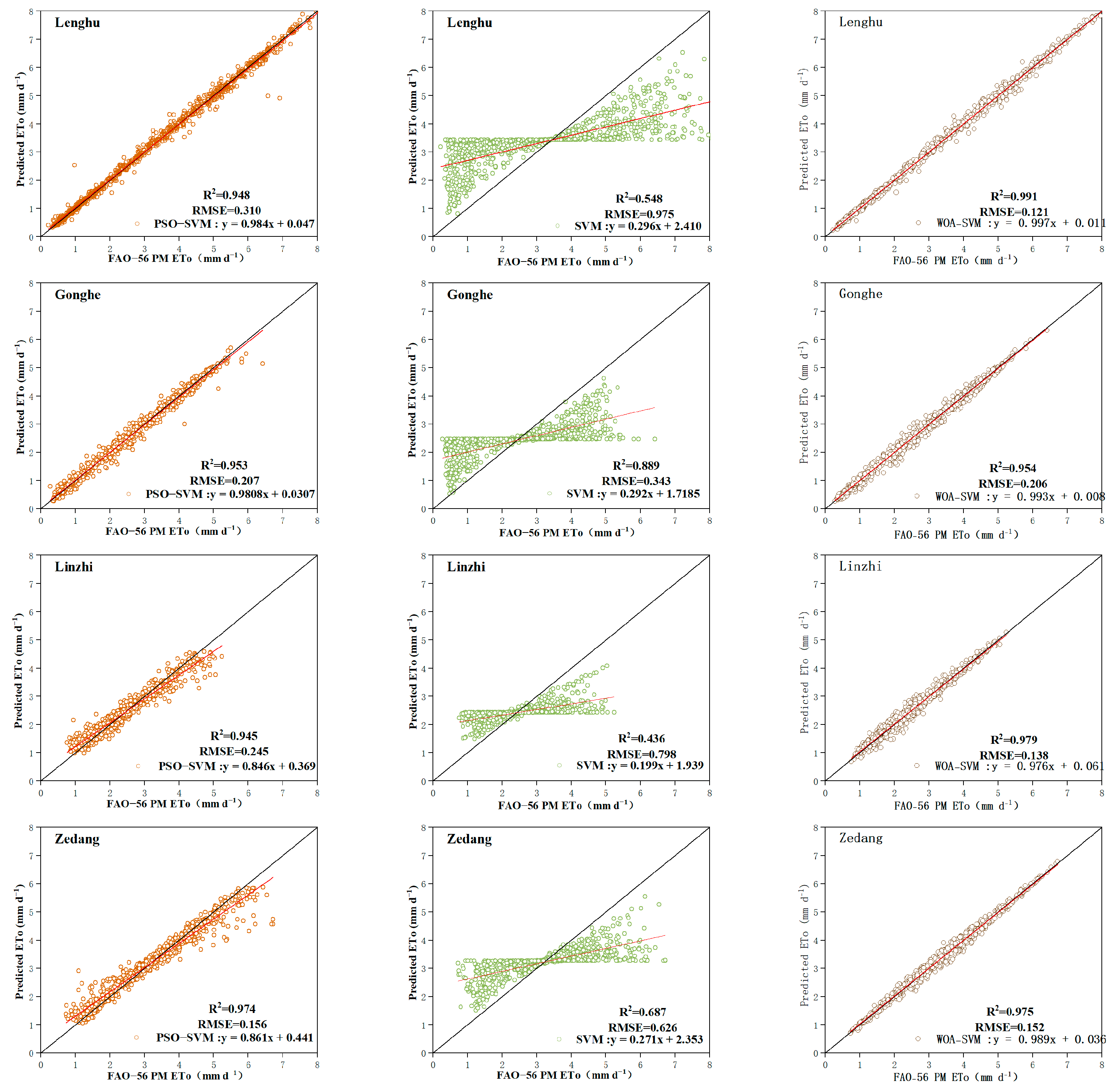
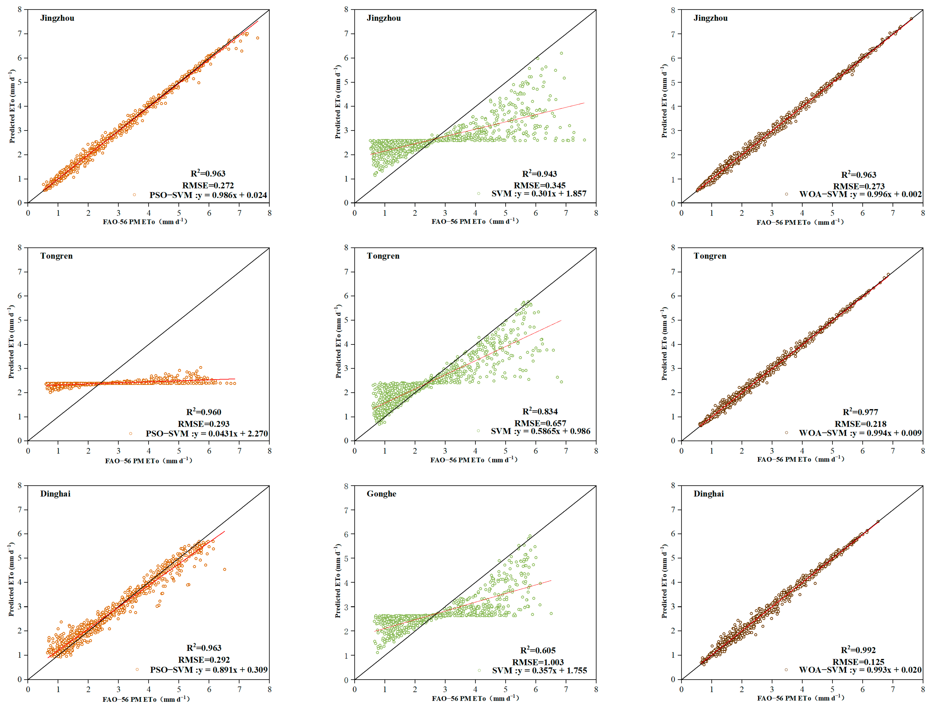
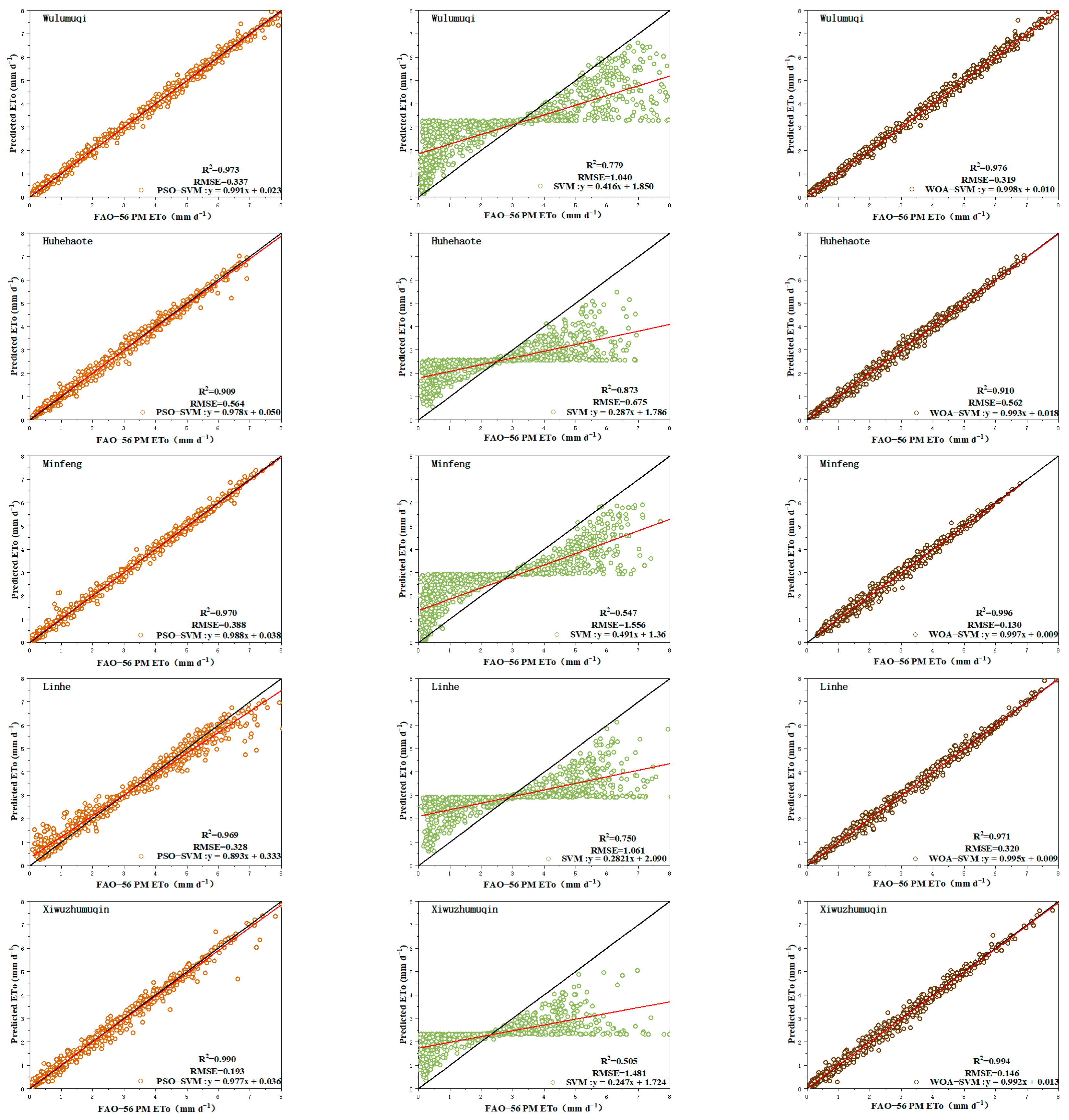
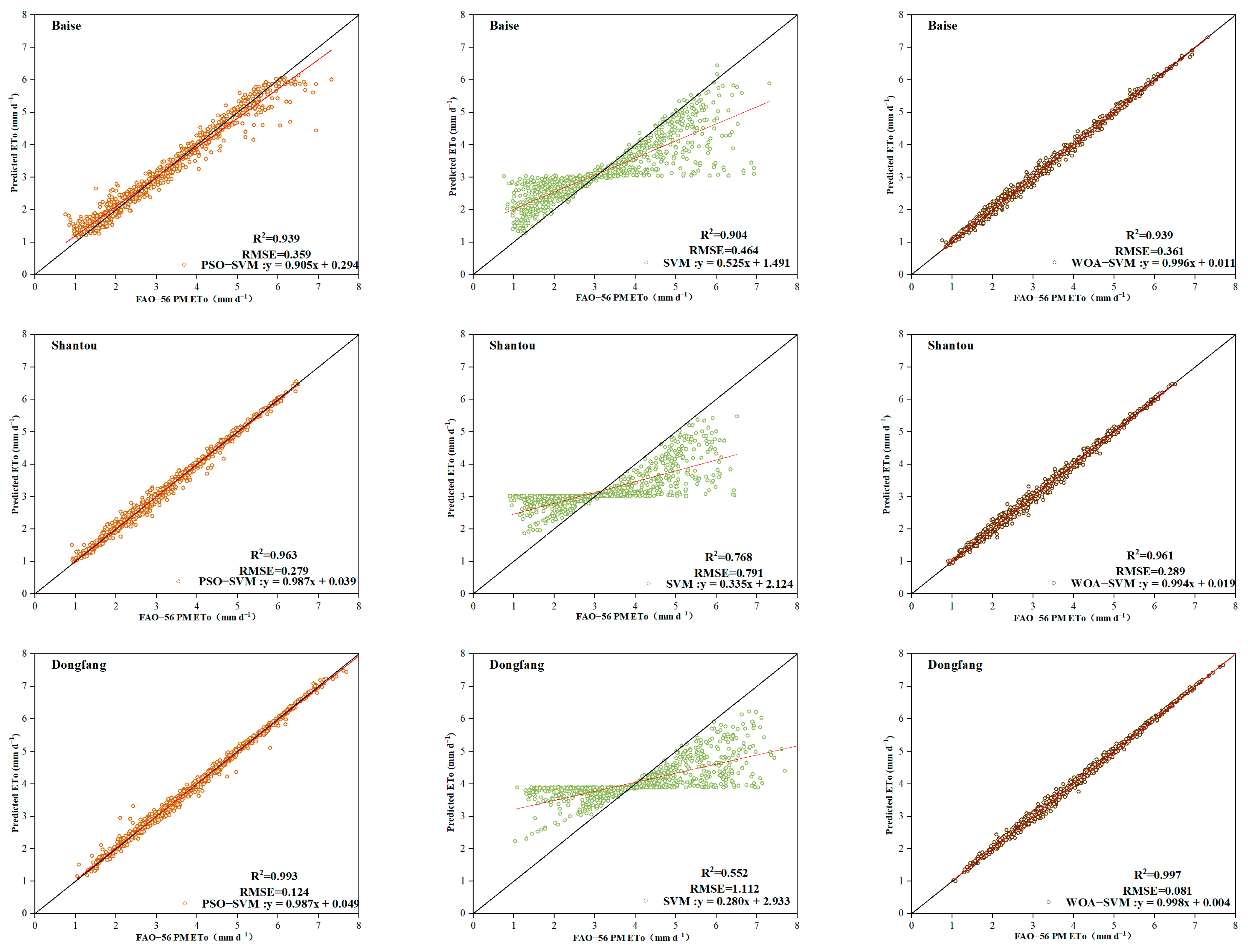
• The WOA-SVM model, which incorporates the WOA for feature selection and parameter tuning, demonstrated the highest accuracy in estimating daily ET₀ across all climatic zones. It outperformed both the PSO-SVM and the standalone SVM models, with the highest R² values observed in the testing phase.
• The PSO-SVM model showed a significant improvement in accuracy compared to the standalone SVM model, indicating the beneficial effect of PSO in enhancing the SVM’s performance. However, it was consistently surpassed by the WOA-SVM model, suggesting the WOA’s potential superiority in optimizing SVM parameters.
• The standalone SVM model, while providing competent results, exhibited comparatively higher RMSE and MAE values and lower R² and NSE values across the training and testing phases, indicating its performance was less accurate than the hybrid models.
• When limited meteorological factors are used to construct the estimation model of ET₀, the model still performs well.

In conclusion, the WOA-SVM model’s consistent outperformance across different climatic zones, its enhanced accuracy through the WOA, and its robust predictive capabilities, even with limited meteorological data, make it a valuable tool for daily ET₀ estimation. The results underscore the potential of machine learning models, particularly when coupled with sophisticated optimization techniques, for advancing water resource management and climate modeling in various climatic contexts. In recent years, the use of drones equipped with multispectral cameras for inverting agricultural parameters in research areas has become a prevalent research topic. Future studies will entail combining multispectral remote sensing and machine learning models to establish a more accurate estimation model. We will also calculate crop water needs and assess the effectiveness of various ET₀ estimation models in optimizing agricultural irrigation systems in subsequent research.

References

1. Gao, H.; Guo, R.; Shi, K.; Yue, H.; Zu, S.; Li, Z.; Zhang, X. Effect of different water treatments in soil-plant-atmosphere continuum based on intelligent weighing systems. Water 2022, 14, 673. [Google Scholar] [CrossRef]
2. Ahmad, L.; Parvaze, S.; Parvaze, S.; Kanth, R. Reference evapotranspiration and crop water requirement of apple (Malus pumila) in Kashmir valley. J. Agrometeorol. 2017, 19, 262–264. [Google Scholar] [CrossRef]
3. Maček, U.; Bezak, N.; Šraj, M. Reference evapotranspiration changes in Slovenia, Europe. Agric. For. Meteorol. 2018, 260, 183–192. [Google Scholar] [CrossRef]
4. Zhao, L.; Zhao, X.; Zhou, H.; Wang, X.; Xing, X. Prediction model for daily reference crop evapotranspiration based on hybrid algorithm and principal components analysis in Southwest China. Comput. Electron. Agric. 2021, 190, 106424. [Google Scholar] [CrossRef]
5. Jeon, M.-G.; Nam, W.-H.; Mun, Y.-S.; Yoon, D.-H.; Yang, M.-H.; Lee, H.-J.; Shin, J.-H.; Hong, E.-M.; Zhang, X. Climate change impacts on reference evapotranspiration in South Korea over the recent 100 years. Theor. Appl. Climatol. 2022, 150, 309–326. [Google Scholar] [CrossRef]
6. Rahman, M.A.; Ali, M.; Mojid, M.A.; Anjum, N.; Haq, M.E.; Kainose, A.; Dissanayaka, K. Crop coefficient, reference crop evapotranspiration and water demand of dry-season Boro rice as affected by climate variability: A case study from northeast Bangladesh. Irrig. Drain. 2023, 72, 148–165. [Google Scholar] [CrossRef]
7. Su, L.; Wang, Q.; Bai, Y. An analysis of yearly trends in growing degree days and the relationship between growing degree day values and reference evapotranspiration in Turpan area, China. Theor. Appl. Clim. 2013, 113, 711–724. [Google Scholar] [CrossRef]
8. El-Kenawy, E.-S.M.; Zerouali, B.; Bailek, N.; Bouchouich, K.; Hassan, M.A.; Almorox, J.; Kuriqi, A.; Eid, M.; Ibrahim, A. Improved weighted ensemble learning for predicting the daily reference evapotranspiration under the semi-arid climate conditions. Environ. Sci. Pollut. Res. 2022, 29, 81279–81299. [Google Scholar] [CrossRef] [PubMed]
9. Gowda, P.H.; Howell, T.A.; Baumhardt, R.L.; Porter, D.O.; Marek, T.H.; Nangia, V. A user-friendly interactive tool for estimating reference ET using ASCE standardized Penman-Monteith equation. Appl. Eng. Agric. 2016, 32, 383–390. [Google Scholar]
10. Zhao, L.; Qing, S.; Bai, J.; Hao, H.; Li, H.; Shi, Y.; Xing, X.; Yang, R. A hybrid optimized model for predicting evapotranspiration in early and late rice based on a categorical regression tree combination of key influencing factors. Comput. Electron. Agric. 2023, 211, 108031. [Google Scholar] [CrossRef]
11. Tao, H.; Diop, L.; Bodian, A.; Djaman, K.; Ndiaye, P.M.; Yaseen, Z.M. Reference evapotranspiration prediction using hybridized fuzzy model with firefly algorithm: Regional case study in Burkina Faso. Agric. Water Manag. 2018, 208, 140–151. [Google Scholar] [CrossRef]
12. Dong, J.; Liu, X.; Huang, G.; Fan, J.; Wu, L.; Wu, J. Comparison of four bio-inspired algorithms to optimize KNEA for predicting monthly reference evapotranspiration in different climate zones of China. Comput. Electron. Agric. 2021, 186, 106211. [Google Scholar] [CrossRef]
13. Gao, L.; Gong, D.; Cui, N.; Lv, M.; Feng, Y. Evaluation of bio-inspired optimization algorithms hybrid with artificial neural network for reference crop evapotranspiration estimation. Comput. Electron. Agric. 2021, 190, 106466. [Google Scholar] [CrossRef]
14. Nagappan, M.; Gopalakrishnan, V.; Alagappan, M. Prediction of reference evapotranspiration for irrigation scheduling using machine learning. Hydrol. Sci. J. 2020, 65, 2669–2677. [Google Scholar] [CrossRef]
15. Ruiming, F.; Shijie, S. Daily reference evapotranspiration prediction of Tieguanyin tea plants based on mathematical morphology clustering and improved generalized regression neural network. Agric. Water Manag. 2020, 236, 106177. [Google Scholar] [CrossRef]
16. Ferreira, L.B.; da Cunha, F.F.; de Oliveira, R.A.; Fernandes Filho, E.I. Estimation of reference evapotranspiration in Brazil with limited meteorological data using ANN and SVM—A new approach. J. Hydrol. 2019, 572, 556–570. [Google Scholar] [CrossRef]
17. Lu, Y.; Li, T.; Hu, H.; Zeng, X. Short-term prediction of reference crop evapotranspiration based on machine learning with different decomposition methods in arid areas of China. Agric. Water Manag. 2023, 279, 108175. [Google Scholar] [CrossRef]
18. Spontoni, T.A.; Ventura, T.M.; Palácios, R.S.; Curado, L.F.; Fernandes, W.A.; Capistrano, V.B.; Fritzen, C.L.; Pavão, H.G.; Rodrigues, T.R. Evaluation and modelling of reference evapotranspiration using different machine learning techniques for a brazilian tropical savanna. Agronomy 2023, 13, 2056. [Google Scholar] [CrossRef]
19. Zhao, Z.; Feng, G.; Zhang, J. The simplified hybrid model based on BP to predict the reference crop evapotranspiration in Southwest China. PLoS ONE 2022, 17, e0269746. [Google Scholar] [CrossRef] [PubMed]
20. Chia, M.Y.; Huang, Y.F.; Koo, C.H. Swarm-based optimization as stochastic training strategy for estimation of reference evapotranspiration using extreme learning machine. Agric. Water Manag. 2021, 243, 106447. [Google Scholar] [CrossRef]
21. Shaloo; Kumar, B.; Bisht, H.; Rajput, J.; Mishra, A.K.; TM, K.K.; Brahmanand, P.S. Reference evapotranspiration prediction using machine learning models: An empirical study from minimal climate data. Agron. J. 2024, 116, 956–972. [Google Scholar] [CrossRef]
22. Youssef, M.A.; Peters, R.T.; El-Shirbeny, M.; Abd-ElGawad, A.M.; Rashad, Y.M.; Hafez, M.; Arafa, Y. Enhancing irrigation water management based on ETo prediction using machine learning to mitigate climate change. Cogent Food Agric. 2024, 10, 2348697. [Google Scholar] [CrossRef]
23. Gupta, S.; Kumar, P.; Kishore, G.; Ali, R.; Al-Ansari, N.; Vishwakarma, D.K.; Kuriqi, A.; Pham, Q.B.; Kisi, O.; Heddam, S. Sensitivity of daily reference evapotranspiration to weather variables in tropical savanna: A modelling framework based on neural network. Appl. Water Sci. 2024, 14, 138. [Google Scholar] [CrossRef]
24. Abdullah, S.S.; Malek, M.A.; Abdullah, N.S.; Kisi, O.; Yap, K.S. Extreme learning machines: A new approach for prediction of reference evapotranspiration. J. Hydrol. 2015, 527, 184–195. [Google Scholar] [CrossRef]
25. Zhu, B.; Feng, Y.; Gong, D.; Jiang, S.; Zhao, L.; Cui, N. Hybrid particle swarm optimization with extreme learning machine for daily reference evapotranspiration prediction from limited climatic data. Comput. Electron. Agric. 2020, 173, 105430. [Google Scholar] [CrossRef]
26. Gatera, A.; Kuradusenge, M.; Bajpai, G.; Mikeka, C.; Shrivastava, S. Comparison of random forest and support vector machine regression models for forecasting road accidents. Sci. Afr. 2023, 21, e01739. [Google Scholar] [CrossRef]
27. Nourani, V.; Elkiran, G.; Abdullahi, J. Multi-step ahead modeling of reference evapotranspiration using a multi-model approach. J. Hydrol. 2020, 581, 124434. [Google Scholar] [CrossRef]
28. Guo, X.; Sun, X.; Ma, J. Prediction of daily crop reference evapotranspiration (ET0) values through a least-squares support vector machine model. Hydrol. Res. 2011, 42, 268–274. [Google Scholar] [CrossRef]
29. Khairan, H.E.; Zubaidi, S.L.; Raza, S.F.; Hameed, M.; Al-Ansari, N.; Ridha, H.M. Examination of Single-and Hybrid-Based Metaheuristic Algorithms in ANN Reference Evapotranspiration Estimating. Sustainability 2023, 15, 14222. [Google Scholar] [CrossRef]
30. Roy, D.K.; Sarkar, T.K.; Biswas, S.K.; Datta, B. Generalized daily reference evapotranspiration models based on a hybrid optimization algorithm tuned fuzzy tree approach. Water Resour. Manag. 2023, 37, 193–218. [Google Scholar] [CrossRef]
31. Ikram, R.M.A.; Mostafa, R.R.; Chen, Z.; Islam, A.R.M.T.; Kisi, O.; Kuriqi, A.; Zounemat-Kermani, M. Advanced hybrid metaheuristic machine learning models application for reference crop evapotranspiration prediction. Agronomy 2022, 13, 98. [Google Scholar] [CrossRef]
32. Zheng, Y.; Zhang, L.; Hu, X.; Zhao, J.; Dong, W.; Zhu, F.; Wang, H. Multi-Algorithm Hybrid Optimization of Back Propagation (BP) Neural Networks for Reference Crop Evapotranspiration Prediction Models. Water 2023, 15, 3718. [Google Scholar] [CrossRef]
33. He, H.; Liu, L.; Zhu, X. Optimization of extreme learning machine model with biological heuristic algorithms to estimate daily reference evapotranspiration in Hetao Irrigation District of China. Eng. Appl. Comput. Fluid Mech. 2022, 16, 1939–1956. [Google Scholar] [CrossRef]
34. Jia, W.; Zhang, Y.; Wei, Z.; Zheng, Z.; Xie, P. Daily reference evapotranspiration prediction for irrigation scheduling decisions based on the hybrid PSO-LSTM model. PLoS ONE 2023, 18, e0281478. [Google Scholar] [CrossRef] [PubMed]
35. Wu, Z.; Chen, X.; Cui, N.; Zhu, B.; Gong, D.; Han, L.; Xing, L.; Zhen, S.; Li, Q.; Liu, Q.; et al. Optimized empirical model based on whale optimization algorithm for simulate daily reference crop evapotranspiration in different climatic regions of China. J. Hydrol. 2022, 612, 128084. [Google Scholar] [CrossRef]
36. Wu, L.; Huang, G.; Fan, J.; Ma, X.; Zhou, H.; Zeng, W. Hybrid extreme learning machine with meta-heuristic algorithms for monthly pan evaporation prediction. Comput. Electron. Agric. 2020, 168, 105115. [Google Scholar] [CrossRef]
37. Long, Z.; Xinbo, Z.; Yuanze, L.; Yi, S.; Hanmi, Z.; Xiuzhen, L.; Xiaodong, W.; Xuguang, X. Applicability of hybrid bionic optimization models with kernel-based extreme learning machine algorithm for predicting daily reference evapotranspiration: A case study in arid and semiarid regions, China. Environ. Sci. Pollut. Res. Int. 2022, 30, 22396–22412. [Google Scholar]
38. Xing, X.; Liu, Y.; Zhao, W.G.; Kang, D.G.; Yu, M.; Ma, X. Determination of dominant weather parameters on reference evapotranspiration by path analysis theory. Comput. Electron. Agric. 2016, 120, 10–16. [Google Scholar] [CrossRef]
39. Pijush Samui, P.S.; Dixon, B. Application of support vector machine and relevance vector machine to determine evaporative losses in reservoirs. Hydrol. Process. 2012, 26, 1361–1369. [Google Scholar] [CrossRef]
40. Pal, M. Support vector machines-based modelling of seismic liquefaction potential. Int. J. Numer. Anal. Methods Geomech. 2006, 30, 983–996. [Google Scholar] [CrossRef]
41. Qiu, Y.; Zhou, J.; Khandelwal, M.; Yang, H.; Yang, P.; Li, C. Performance evaluation of hybrid WOA-XGBoost, GWO-XGBoost and BO-XGBoost models to predict blast-induced ground vibration. Eng. Comput. 2022, 38, 4145–4162. [Google Scholar] [CrossRef]
42. Deghfel, N.; Badoud, A.E.; Merahi, F.; Bajaj, M.; Zaitsev, I. A new intelligently optimized model reference adaptive controller using GA and WOA-based MPPT techniques for photovoltaic systems. Sci. Rep. 2024, 14, 6827. [Google Scholar] [CrossRef] [PubMed]
43. Tikhamarine, Y.; Malik, A.; Pandey, K.; Sammen, S.S.; Souag-Gamane, D.; Heddam, S.; Kisi, O. Monthly evapotranspiration estimation using optimal climatic parameters: Efficacy of hybrid support vector regression integrated with whale optimization algorithm. Environ. Monit. Assess. 2020, 192, 696. [Google Scholar] [CrossRef] [PubMed]
44. Feng, Y.; Cui, N.; Zhao, L.; Hu, X.; Gong, D. Comparison of ELM, GANN, WNN and empirical models for estimating reference evapotranspiration in humid region of Southwest China. J. Hydrol. 2016, 536, 376–383. [Google Scholar] [CrossRef]
45. Yong, S.L.S.; Ng, J.L.; Huang, Y.F.; Ang, C.K.; Ahmad Kamal, N.; Mirzaei, M.; Najah Ahmed, A. Enhanced daily reference evapotranspiration estimation using optimized hybrid support vector regression models. Water Resour. Manag. 2024, 1–29. [Google Scholar] [CrossRef]
46. Li, S.; Fan, Z. Evaluation of urban green space landscape planning scheme based on PSO-BP neural network model. Alex. Eng. J. 2022, 61, 7141–7153. [Google Scholar] [CrossRef]
47. Liang, F.; Sun, L.; Zeng, Z.; Kang, J. Treatment of surfactant wastewater by foam separation: Combining the RSM method and WOA-BP neural network to explore optimal process conditions. Chem. Eng. Res. Des. 2023, 193, 85–98. [Google Scholar] [CrossRef]
48. Lian, Z.; Duan, L.; Qiao, Y.; Chen, J.; Miao, J.; Li, M. The improved ELM algorithms optimized by bionic WOA for EEG classification of brain computer interface. IEEE Access 2021, 9, 67405–67416. [Google Scholar] [CrossRef]
49. Figueiredo, E.M.; Ludermir, T.B. Investigating the use of alternative topologies on performance of the PSO-ELM. Neurocomputing 2014, 127, 4–12. [Google Scholar] [CrossRef]
50. Mohammadi, B.; Mehdizadeh, S. Modeling daily reference evapotranspiration via a novel approach based on support vector regression coupled with whale optimization algorithm. Agric. Water Manag. 2020, 237, 106145. [Google Scholar] [CrossRef]
51. Feng, Y.; Gong, D.; Zhang, Q.; Jiang, S.; Zhao, L.; Cui, N. Evaluation of temperature-based machine learning and empirical models for predicting daily global solar radiation. Energy Convers. Manag. 2019, 198, 111780. [Google Scholar] [CrossRef]
52. Shiri, J.; Nazemi, A.H.; Sadraddini, A.A.; Landeras, G.; Kisi, O.; Fard, A.F.; Marti, P. Comparison of heuristic and empirical approaches for estimating reference evapotranspiration from limited inputs in Iran. Comput. Electron. Agric. 2014, 108, 230–241. [Google Scholar] [CrossRef]
Figure 1. Geographical locations of the 18 weather stations across the different climatic zones of China.
Agronomy 14 01780 g001
Figure 2. Technical route in this study.
Agronomy 14 01780 g002
Figure 3. Fitting performance of the daily ET0 estimation models in MPZ.
Agronomy 14 01780 g003
Figure 4. Fitting performance of the daily ET0 estimation models in SMZ.
Agronomy 14 01780 g004
Figure 5. Fitting performance of the daily ET0 estimation models in TCZ.
Agronomy 14 01780 g005
Figure 6. Fitting performance of the daily ET0 estimation models in TMZ.
Agronomy 14 01780 g006
Figure 7. Fitting performance of the daily ET0 estimation models in TMPZ.
Agronomy 14 01780 g007