Article

A Hybrid Synthetic Minority Oversampling Technique and Deep Neural Network Framework for Improving Rice Yield Estimation in an Open Environment

1
College of Information Science & Technology, Hebei Agricultural University, Baoding 071001, China
2
Academy of National Food and Strategic Reserves Administration, Beijing 100037, China
3
Agricultural Technology Promotion Center of Beidahuang Agriculture Co., Ltd. 290 Branch, Suihua 156202, China
4
Big Data Development Center, Ministry of Agriculture and Rural Affairs, Beijing 100125, China
5
Agriculture Information Institute, Chinese Academy of Agriculture Science, Beijing 100086, China
*
Author to whom correspondence should be addressed.
Agronomy 2024, 14(9), 1890; https://doi.org/10.3390/agronomy14091890
Submission received: 7 August 2024 / Revised: 20 August 2024 / Accepted: 23 August 2024 / Published: 24 August 2024
(This article belongs to the Section Precision and Digital Agriculture)

Abstract

:
Quick and accurate prediction of crop yields is beneficial for guiding crop field management and genetic breeding. This paper utilizes the fast and non-destructive advantages of an unmanned aerial vehicle equipped with a multispectral camera to acquire spatial characteristics of rice and conducts research on yield estimation in an open environment. The study proposes a yield estimation framework that hybrids synthetic minority oversampling technique (SMOTE) and deep neural network (DNN). Firstly, the framework used the Pearson correlation coefficient to select 10 key vegetation indices and determine the optimal feature combination. Secondly, it created a dataset for data augmentation through SMOTE, addressing the challenge of long data collection cycles and small sample sizes caused by long growth cycles. Then, based on this dataset, a yield estimation model was trained using DNN and compared with partial least squares regression (PLSR), support vector regression (SVR), and random forest (RF). The experimental results indicate that the hybrid framework proposed in this study performs the best (R2 = 0.810, RMSE = 0.69 t/ha), significantly improving the accuracy of yield estimation compared to other methods, with an R2 improvement of at least 0.191. It demonstrates that the framework proposed in this study can be used for rice yield estimation. Additionally, it provides a new approach for future yield estimation with small sample sizes for other crops or for predicting numerical crop indicators.

1. Introduction

China is a major agricultural country in the world. The growing population leads to a continuous increase in the demand for food. As one of the primary food crops, rice plays an essential role in ensuring the supply of food. Rapid and accurate estimation of rice yield can effectively guide field management and genetic breeding, further enhancing rice productivity and ensuring food security. Therefore, conducting research on rice yield estimation is of great significance.
Traditional rice yield estimation requires the determination of panicle number, grain number per panicle, and thousand-grain weight, which is time-consuming and labor-intensive and also requires destructive sampling. In response, researchers have developed crop growth models such as WOFOST [1], DSSAT [2], and APSIM [3]. To achieve better yield estimation results, these models require a large amount of crop growth parameters, soil data, and meteorological data, which undoubtedly increases the complexity and cost of yield estimation.
Remote sensing, as a non-contact technology for detecting targets, has been widely applied in the field of agriculture. Models for estimating aboveground biomass [4] and leaf area index [5] have been established based on satellite remote sensing data, enabling the monitoring of crop growth in the field. Yuan et al. [6] utilized the spatial continuity characteristic of satellite remote sensing to obtain crop disease features, thereby enhancing disease monitoring capabilities. Of course, research has also been conducted in the field of yield estimation. For example, Gómez et al. [7] combined satellite remote sensing with climate data to achieve regional wheat yield estimation by inverting soil moisture, leaf area index, and other related parameters from satellite remote sensing data and assimilating them into crop growth models, improving the accuracy of winter wheat yield estimation [8,9]. However, the acquisition of satellite remote sensing data is greatly affected by weather conditions, and due to high costs and low spatial resolution, there are significant difficulties in the continuous acquisition of data [10,11].
In recent years, unmanned aerial vehicles (UAVs) have been widely applied in the fields of geology [12], transportation [13], and agriculture [14] thanks to their advantages such as speed, non-destructiveness, and low cost. By carrying sensors, UAVs can quickly acquire spatial, temporal, and spectral characteristics of the research targets, providing more reliable data support for studies. In terms of yield estimation, Yang et al. [15] utilized hyperspectral cameras mounted on UAVs to capture images and models by integrating spectral information with spatial image information. Compared to single types of features, multiple types of features can effectively enhance the performance of corn yield estimation. During the rice ripening period, Tanaka et al. [16] used digital cameras mounted on UAVs under different lighting conditions and different shooting angles to obtain RGB images, achieving rapid yield estimation (R2 = 0.686, rRMSE = 0.22). However, the acquisition of RGB images is greatly affected by the growth time of crops and shooting angles, and the cost of acquiring hyperspectral images is relatively high. In contrast, multispectral images are more conveniently obtained, allowing data collection throughout the entire growth period of crops with lower costs, overcoming the difficulties and deficiencies in the acquisition of RGB and hyperspectral images; thus, it has been favored in yield estimation research. For example, Fu et al. [17] used multispectral vegetation indices (VIs) and established a wheat yield prediction model with six machine learning algorithms, achieving the best performance with R2 = 0.78 and rRMSE = 0.103. Marques Ramos et al. [18] ranked the importance of multispectral Vis, selected the top three index features as model inputs, and built a corn yield estimation model based on the random forest algorithm, with an estimation accuracy of R2 = 0.78 and MAE = 853.11 kg/ha. Of course, in order to obtain more accurate yield estimation results, multimodal features have received widespread attention. Pukrongta et al. [19], Ma et al. [20], and Mia et al. [21] have all used the multimodal concept to carry out crop yield prediction and achieved good results, proving that multimodal data has greater advantages than single-modal data.
Crop yield prediction is an emerging topic in the field of precision agriculture research. However, the data collection cycle is long, and generally, data can only be collected once a year, leading to a limited number of data samples. In response to this issue, few researchers have proposed solutions, and the size of the dataset is crucial for modeling based on machine learning algorithms. Therefore, in this study, rice experiments were set up in an open environment with multiple varieties, planting densities, and base fertilizer amounts. Rice yield estimation research was conducted based on the multispectral information for the experimental fields. The main contributions are as follows:
  • A combination of rice yield estimation features was established using the Pearson correlation coefficient.
  • SMOTE was introduced to address the issue of insufficient data samples, fully leveraging the advantages of machine learning algorithms and enhancing the accuracy of yield estimation.
  • A hybrid SMOTE and DNN framework for rice yield estimation was established.
The rest of this paper is structured as follows. Section 2 describes the research area and settings and provides a detailed introduction to the process of data acquisition and processing, as well as the methods used in the study. In Section 3, the experimental results are presented and discussed. Finally, in Section 4, the results of this study are summarized.

2. Materials and Methods

2.1. Study Area

The experimental fields are located in Heilongjiang Province, China (132°08′ E, 47°57′ N), with three gradients of different varieties, planting densities, and base fertilizer amounts, in a total of 10 plots. (For specific information, see Table 1). Since the experimental fields are for rice growing in an open environment, they are not the standard experimental fields in the traditional sense. Therefore, the plot sizes are not completely identical. During the crop growth process, field management is maintained at the best level according to the local agricultural operation standards. The basic situation of the study area is shown in Figure 1.

2.2. UAV Image Collection

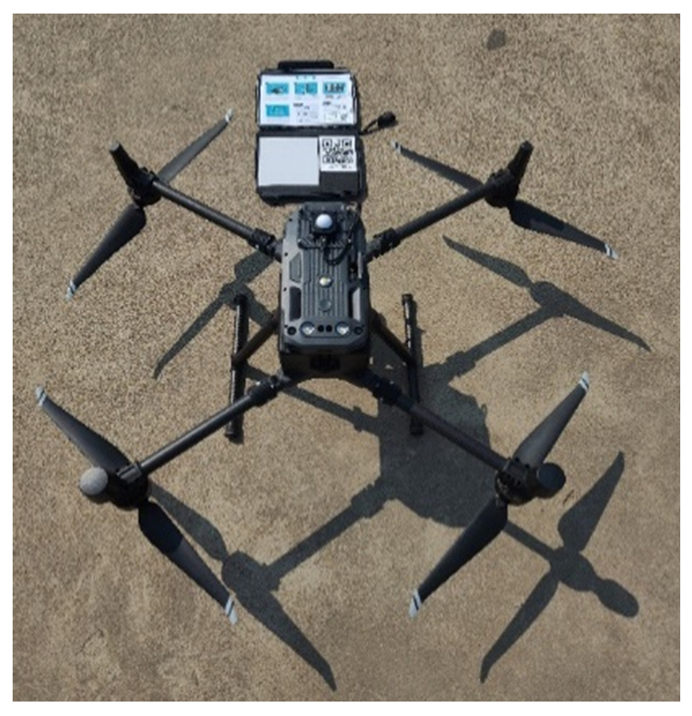
This paper uses the DJI M300 RTK (SZ DJI Technology Co., Ltd., Guangdong, China) equipped with a multispectral sensor (MS600 Pro (SZ DJI Technology Co., Ltd., Guangdong, China)) and an RGB sensor (Zenmuse P1 (SZ DJI Technology Co., Ltd., Guangdong, China)) to collect experimental field image data, as shown in Figure 2. The MS600 Pro includes 6 spectral channels: Blue, Green, Red, Red Edge 1, Red Edge 2, and Near-Infrared, with detailed information provided in Table 2.

2.2.1. Multispectral Image

During the milk ripening stage of rice, multispectral images are collected using the MS600 Pro mounted on a UAV to obtain the spectral reflectance of the rice canopy. The UAV flies at an altitude of 30 m, with a heading overlap rate of 80% and a lateral overlap rate of 70%, and the camera takes photos in a mode with equal time intervals perpendicular to the ground. To accurately acquire the spectral reflectance, we pay more attention to two points:
  • Before data collection, reflectance calibration is carried out using a calibration plate, as shown in Figure 3.
  • The flight is conducted under cloudless and well-lit conditions (from 10:00 to 14:00 Beijing time in China).

2.2.2. RGB Images

The RGB images are collected after the rice has matured and the sample points have been manually harvested. The main purpose is to accurately locate the area of study to facilitate the extraction of spectral reflectance. Specifically, RGB images are captured using a Zenith P1 camera mounted on a UAV, with the same parameters and shooting time as for multispectral image acquisition.

2.3. Yield Data Collection

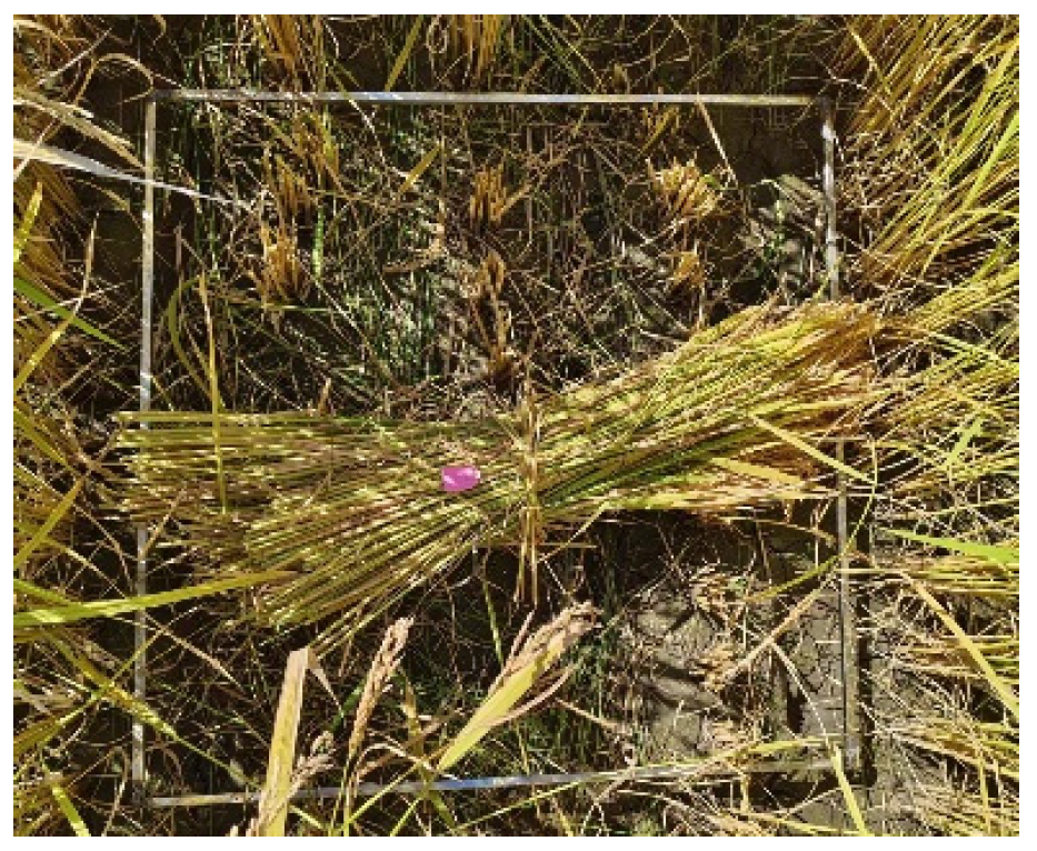
After the rice matures, we use a standard of 1 m2 (1 m × 1 m) as sample points, randomly selecting sample points in the experimental fields for manual harvesting and sampling. Each sample point is used as a unit for drying, threshing, and weighing to obtain yield data, with a total of 293 sample areas collected. Figure 4 shows the situation when harvesting a sample point, with each sample point’s rice bundled and marked with a tag.

2.4. Image Processing

After completing data collection using the UAV, (1) Pix 4D (Pix4D SA, Lausanne, Switzerland) is used to stitch the images to obtain orthophotos. (2) QGIS is used to delineate the regions of interest (ROI) on the RGB images, a process that is based on establishing shapefile vector files while also assigning an ID to represent different sample points. (3) After matching the sample area markings with multispectral images, spectral reflectance extraction and VI calculations are conducted (the spectral reflectance values in this paper are taken as the average value of each pixel at each sample point).

2.5. Method

This study has established a rice yield estimation framework based on SMOTE and DNN, as shown in Figure 5. (1) Data acquisition and preprocessing. (2) Data augmentation and model training. (3) Model evaluation and instance verification.
The section on data acquisition and preprocessing has been introduced in detail in the previous chapters. It is worth noting that we divided the data into training data and testing data for easy fusion with the data augmentation later on. In the data augmentation part, we introduced the SMOTE to expand the samples of the minority class, obtaining an augmented dataset. To ensure the applicability of SMOTE, this study divides the data into three categories to create the original dataset based on the amount of rice yield for each sample point, as shown in Table 3. The augmented dataset was divided into training data and test data. The divided dataset was then merged with the original data to form the training and test data required for modeling, ensuring a uniform distribution of samples. Subsequently, a yield estimation model was established using DNN, and the entire original dataset was used to test the model to verify the effectiveness of data augmentation. After the model is established, we can estimate the yield by inputting new feature data.

2.5.1. Selection of VIs

By reviewing a large amount of literature, we extracted 53 VIs from multispectral reflectance (for details, see Appendix A). We conducted feature analysis using the Pearson correlation coefficient, and the correlation of each index with yield is shown in Figure 6.
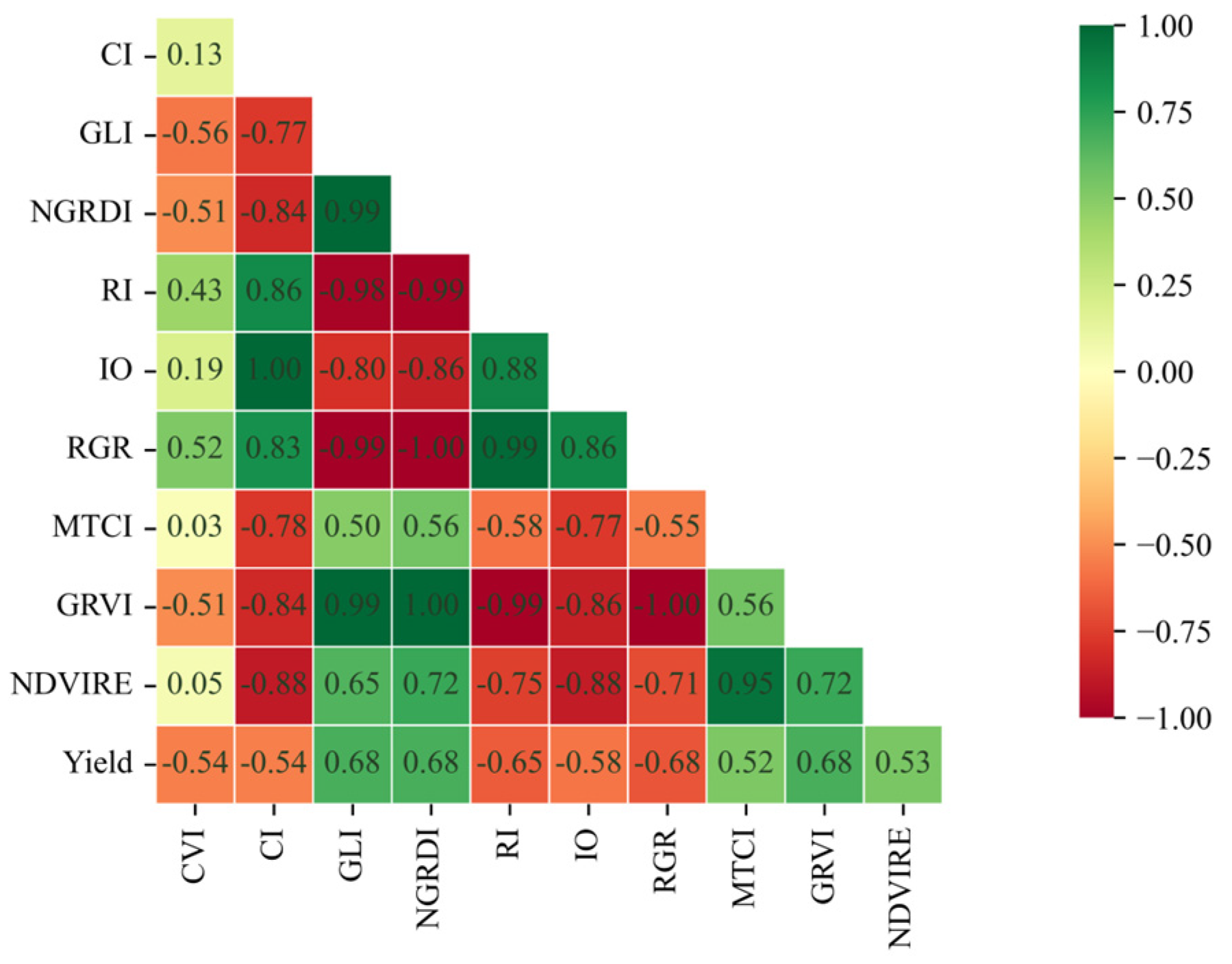
We selected 10 vegetation indices with strong correlations with yield as input features for the yield estimation model. The correlation heatmap is shown in Figure 7, with all correlation coefficients having absolute values greater than 0.5. Table 4 describes each VI we used and its calculation formula.

2.5.2. Data Augmentation

For machine learning modeling, the size of the dataset is crucial to the quality of the model; the more data points available, the better the model performs and the stronger its generalization capability. Conversely, a lack of data can lead to poor generalization. Therefore, in situations with limited data, it is necessary to augment the dataset. In the field of image recognition, data augmentation is often achieved through methods such as image rotation, scaling, and color transformation. In this study, we introduce SMOTE to perform data augmentation, addressing the issue of insufficient data samples caused by long data collection cycles. This technique reduces the model’s over-reliance on certain features and enhances the learning of characteristics from minority classes, thereby improving the model’s generalization and accuracy.
SMOTE [22], introduced by Chawla in 2002, has been extensively applied in various fields such as clinical data classification [23], earthquake risk assessment [24], and air quality forecasting [25]. The fundamental concept involves selecting a sample from the minority class, denoted as x , identifying k nearest neighbor samples within that class, and then randomly selecting one of those nearest neighbors, denoted as x ~ . A new sample is generated using the following formula, where a is a random number between 0 and 1.
x n e w = x + a x ~ x
Using SMOTE, we performed data augmentation on the original dataset, setting the imbalance rate (IR) to 1.03, which represents the ratio of the number of samples in the majority class to the number of samples in the minority class. In this study, Category II is considered as the positive sample, i.e., the majority class, while Category I and Category III are considered as negative samples I and negative samples II, respectively, i.e., the minority classes, and data augmentation is completed for each. Ultimately, the data increased from the original 293 data points to 424 data points. The dataset obtained after enhancement is shown in Table 5.

2.5.3. DNN Architecture

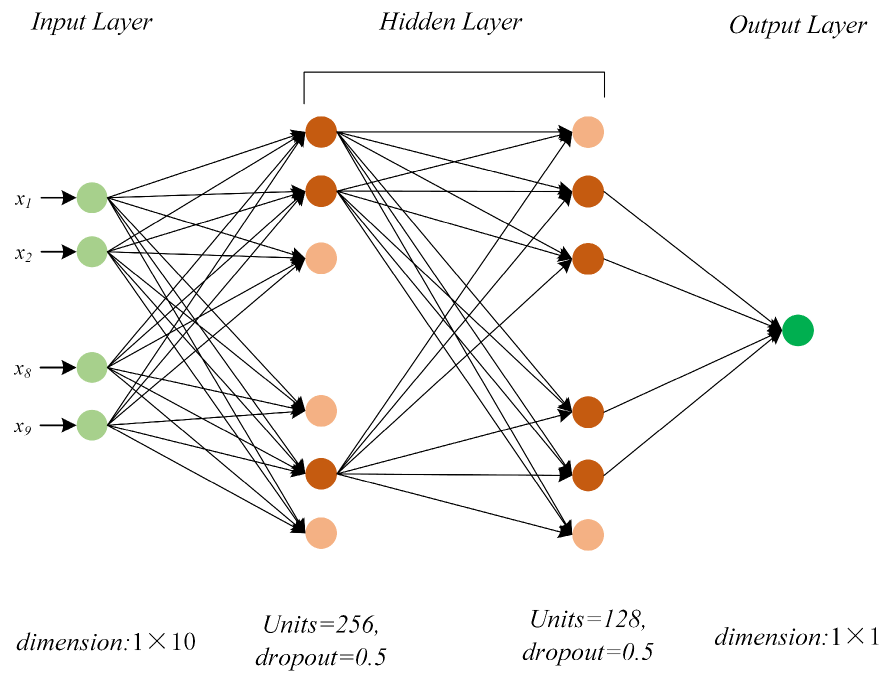
DNN is a type of neural network that has multiple hidden layers, specifically designed to model the complex nonlinear relationships between inputs and outputs. It has achieved significant success in numerous fields such as computer vision, natural language processing, and speech recognition. Figure 8 describes the DNN architecture constructed in this study, which consists of one input layer, two hidden layers, and one output layer. The input layer has a data dimension of 1 × 10, corresponding to the standard values of the features. The neurons in the hidden layers are 256 and 128, respectively, and a Dropout layer is added after each layer, both set to 0.5 (All parameters are determined through an ablation study). The dimension of the output layer is 1, which is the yield value corresponding to the feature.
At the same time, Adam is used as the optimizer, with the learning rate lr = 0.01. The mean squared error (MSE) loss function calculates the error between the network’s predicted values and the actual sample values, as shown in the following formula.
M S E = 1 n i = 1 n ( y i y i ^ ) 2
n represents the number of samples, y i represents the actual value of sample i , and y i ^ represents the predicted value of sample i .

2.5.4. Model Evaluation Criteria

This paper uses the coefficient of determination (R2) and the Root Mean Square Error (RMSE) as model evaluation metrics. The larger the R2, the better the model fits the data, indicating higher prediction accuracy. The smaller the RMSE, the smaller the difference between the predicted values and the actual values, indicating higher prediction accuracy of the model. To prevent overfitting and enhance the generalizability of the model, this paper employs a 5-fold cross-validation, taking the average as the final metric for evaluation.
R 2 = 1 i = 1 n y i ^ y i 2 i = 1 n y i ¯ y i 2
R M S E = 1 n i = 1 n ( y i y i ^ ) 2
n represents the number of samples, y i represents the actual value of sample i , y i ^ represents the predicted value of sample i , and y i ¯ represents the mean of all the measured yield values.

3. Results

This section introduces the experimental results and summarizes the yield estimation results under different treatments.

3.1. Model Results

Before training the model, we conducted a correlation test on the multispectral VIs. On one hand, this was to further refine feature selection and reduce the feature dimensionality. On the other hand, it was to mitigate the impact of highly correlated indices on the model. In this paper, we calculated the correlations between 53 VIs and yield and selected the top 10 VIs with the highest correlation to yield as inputs for the model, as depicted in Figure 7.
In previous yield estimation studies, the random forest has been proven to have a significant advantage. Therefore, in this study, we used partial least squares regression (PLSR), support vector machine (SVR), random forest (RF), and deep neural networks (DNNs) as four machine learning algorithms to establish a rice yield prediction model in an open environment.
Table 6 presents the yield estimation results for each model without feature selection and data augmentation. It can be seen that DNNs perform the best (R2 = 0.619, RMSE = 0.95 t/ha), followed by RF, PLSR, and SVR.
Table 7 shows the yield estimation results without feature selection but with data augmentation. The result is still that DNNs perform the best (R2 = 0.770, RMSE = 0.73 t/ha), followed by RF, SVR, and PLSR. Comparing the results in Table 6 and Table 7, regardless of the model, shows that the accuracy of yield estimation is improved after data augmentation, with the most significant improvement being in SVR, which is about 33.4%; its results exceed PLSR. This also verifies the importance of data size in machine learning algorithms.
Table 8 shows the yield estimation results without data augmentation after feature selection, with DNN still performing the best (R2 = 0.634, RMSE = 0.93 t/ha). Next come RF, PLSR, and SVR. It has been proven that feature selection not only achieves data dimensionality reduction and algorithm complexity reduction but also maximizes the advantages of features and improves the accuracy of the model. After feature screening, the accuracy is also improved to a certain extent, but the improvement is not significant. The most obvious improvement is SVR, with an increase of about 4.2%, which is significantly different from the improvement in data augmentation.
Table 9 shows the experimental results of feature selection and data augmentation (i.e., within the research framework proposed in this study), with DNN performing the best (R2 = 0.810, RMSE = 0.69 t/ha), followed by RF, SVR, and PLSR. Compared with the results in Table 6, the accuracy of each model is significantly improved, with an increase of over 30%.
In summary, from the above experimental results, we can see that feature selection can also have a positive effect on estimation accuracy, and data augmentation has a greater impact on estimation accuracy, which is consistent with the high dependence of machine learning on datasets. Meanwhile, in traditional machine learning methods, RF performance is indeed the best, consistent with previous research results. Certainly, the prediction performance based on DNN is the best after feature selection and data augmentation, which is the hybrid SMOTE and DNN framework proposed in this study.

3.2. Oversampling Analysis

This article uses 5-fold cross-validation and takes the average as the experimental result to reduce the risk of overfitting and obtain a more reliable yield estimation model. We also compared the DNN results using the training and testing sets, as shown in Table 10. R2 values were all greater than 0.83, but not very close to 1, and the corresponding test set results did not show extreme deviation from the training set results. Therefore, we believe that there was no overfitting phenomenon in this study.

4. Discussion

This section discusses the impact of feature selection, data augmentation, and modeling algorithms on the estimation of rice yield.

4.1. The Impact of Feature Selection on Yield Estimation

Comparing the model performance before and after feature selection, it can be observed that the predictive performance of all models has been improved to varying degrees. Before data augmentation, the R2 increased by 0.015–0.021, and after data augmentation, the R2 increased by 0.029–0.047. This demonstrates that feature selection effectively eliminated redundant features, reduced the complexity of the algorithms, and enhanced algorithm performance while ensuring the accuracy of the predictions. Many studies have also used similar methods for feature selection and achieved good results. For example, Shen et al. [26] used recursive feature elimination (RFE) to determine the optimal feature set for the model, which improved the predictive performance. The results showed that PLSR performed best under the selected features, and extreme gradient boosting (XGBoost) performed best with all features, with R2 both at 0.827. Their results are superior to the results of this study (R2 = 0.810), which we believe is due to the use of hyperspectral data with more bands and richer features. However, the optimal model in their study changed before and after feature selection, and a high-performance yield estimation method was not determined. In contrast, in this study, DNN consistently showed the best performance. Another point worth noting is that their study ultimately selected 15 features, while our study only used 10 features. Another example is Marques Ramos et al. using RF to rank the importance of Vis and selecting the top three features from 33 VIs as inputs, successfully enhancing the yield prediction effect of corn [18]. We also attempted to use RF to replace the Pearson correlation coefficient for feature selection; the results are shown in Table 11. There was an improvement compared with the results before feature selection, and the overall performance was not significantly different from the Pearson correlation coefficient used in this paper. We believe that the feature selection method is strongly correlated with the dataset itself. Therefore, in the research process, it is necessary to try multiple feature selection methods and select the best method for different applications.

4.2. The Impact of Data Augmentation on Yield Estimation

One of the most important aspects of this study is the adoption of data augmentation techniques, which addressed the issue of limited data due to the long growth cycle of crops. It can be clearly seen from Table 6 that the accuracy of yield estimation is significantly improved after SMOTE data augmentation. With all features, the R2 was increased by at least 0.13 (PLSR) and by up to 0.17 (SVR). After feature selection, the R2 was improved by at least 0.16 (PLSR) and by up to 0.18 (SVR and DNN).
SMOTE has been applied in research across various fields [27,28], demonstrating its ability to address the issue of imbalanced datasets, and modeling performance was significantly enhanced after data augmentation using SMOTE. However, these studies are mostly aimed at classification tasks. In studies targeting prediction tasks, it is necessary to appropriately transform the prediction problem into a classification problem and then apply SMOTE to solve the data imbalance issue, thereby improving the prediction effect. For example, in the study of air quality prediction, Ke et al. divided the data into two categories: one is high pollution (minority category) and the other is normal (majority category) [25]. In this study, data are categorized into three classes based on the amount of yield, with Category II as the majority class, and Category I and Category III as the minority classes, achieving data augmentation through SMOTE.

4.3. Study Limitations and Future Work

In this study, we mainly achieved data augmentation through SMOTE to improve the accuracy of rice yield estimation. However, our research also has certain limitations. Firstly, only data from a single growth stage (milk ripening stage) of rice was used, lacking the application of multi-temporal data. Studies [29,30,31] demonstrated that multi-temporal feature yield estimation is superior to single-temporal feature estimation. Secondly, the feature source is singular. The characteristic of this study is the multispectral VIs, and multiple studies have shown that multimodal data are more beneficial for improving the robustness and accuracy of the model. In the research on yield estimation, Mia et al. [21] and Sun et al. [32] conducted research using multimodal features and pointed out that the estimation effect of multimodal features is better than that of single-modal features. Thirdly, feature selection is crucial for machine learning modeling. Although this study compared the Pearson correlation coefficient and RF methods, it did not conduct a comparative analysis of RFE and recursive feature elimination with cross-validation (RFECV), which have also been applied in this field.
In summary, the application of multimodal features and multi-temporal data is the future development trend. In subsequent research, we will collect multispectral and RGB data on rice throughout its growth period, and synchronously collect relevant environmental parameters (such as meteorological data, soil data, etc.) in order to carry out yield estimation using multi-temporal and multimodal data. At the same time, in order to further leverage the optimal features, we will conduct yield estimation research on different growth stages to determine the optimal features for that period, and then use feature weight fusion to achieve multi-temporal and multimodal yield estimation. We believe that this method can effectively improve the accuracy of yield estimation. Of course, SMOTE data augmentation will also be continuously applied.

5. Conclusions

This study proposes a framework for rice yield estimation in an open environment. First, based on previous research, 53 commonly used VIs were selected and 10 features with strong correlations (all correlation coefficients greater than 0.5) were extracted as input features using the Pearson correlation coefficient. Second, the data were categorized into three classes based on the amount of rice yield, and data augmentation was achieved using SMOTE to address the issue of insufficient samples. Finally, the enhanced dataset was used to train a DNN model and compared with PLSR, SVR, and RF. The experimental results demonstrate that (1) regardless of whether feature selection or data augmentation is applied, the yield estimation model established based on DNN outperforms other models. (2) After feature selection, the model’s performance is enhanced, proving that the Pearson correlation coefficient method can effectively eliminate redundant features and reduce algorithmic complexity. (3) The model’s performance is significantly improved after data augmentation (R2 = 0.810, RMSE = 0.69 t/ha), and different baseline algorithms show substantial improvements when modeled based on the augmented dataset, proving that models trained with SMOTE-enhanced data can effectively enhance the accuracy of rice yield estimation, highlighting the advantages of SMOTE data augmentation. The research findings provide strong support for yield estimation and offer new perspectives for future yield estimation of other crops using small sample sizes or for predicting numerical crop indicators.

Author Contributions

Conceptualization, L.G. and J.Y.; methodology, J.Y.; validation, J.Y. and Z.Z.; formal analysis, J.Y.; data curation, Z.Z. and C.C.; writing—original draft preparation, J.Y.; writing—review and editing, L.G. and W.W.; project administration, L.G.; funding acquisition, L.G. All authors have read and agreed to the published version of the manuscript.

Funding

This research was funded by the National Key R&D Program of China, grant number 2021ZD0110901.

Data Availability Statement

The data presented in this study are available upon request from the corresponding author.

Conflicts of Interest

Author Changming Chu was employed by the company Agricultural Technology Promotion Center of Beidahuang Agriculture Co., Ltd. The remaining authors declare that the research was conducted in the absence of any commercial or financial relationships that could be construed as a potential conflict of interest.

Appendix A. Vegetation Indices Extracted in This Paper

Serial NumberVegetation IndexFormulaReference
1ATSAVI (Adjusted Transformed Soil-adjusted Vegetation Index) 1.22 × R n i r 1.22 × R r e d 0.03 1.22 × R n i r + R r e d 1.22 × 0.03 + 0.08 × 1 + 1.22 2 [33]
2ARVI2 (Atmospherically Resistant Vegetation Index2) 0.18 + 1.17 × R n i r R r e d / R n i r + R r e d [33]
3BWDRVI (Blue-wide Dynamic Range Vegetation Index) 0.1 × R n i r R b l u e 0.1 × R n i r + R b l u e [34]
4CCCI (Canopy Chlorophyll Content Index) R n i r R r e d e d g e R n i r + R r e d e d g e / R n i r R r e d R n i r + R r e d [33]
5CIgreen (Chlorophyll Index Green) R n i r / R g r e e n 1 [35]
6CIrededge (Chlorophyll Index RedEdge) R n i r / R r e d e d g e 1 [35]
7CVI (Chlorophyll Vegetation Index) R n i r × R r e d / R g r e e n 2 [33]
8CI (Coloration Index) R r e d R b l u e R r e d [36]
9NDVI (Normalized Difference Vegetation Index) R n i r R r e d R n i r + R r e d [37]
10CTVI (Corrected Transformed Vegetation Index) R n i r R r e d R n i r + R r e d + 0.5 R n i r R r e d R n i r + R r e d + 0.5 [38]
11GDVI (Difference NIR/Green Difference Vegetation Index) R n i r R g r e e n [33]
12EVI (Enhanced Vegetation Index) R n i r R r e d R n i r + 6 × R r e d 7.5 × R b l u e + 1 [39]
13EVI2 (2-band Enhanced Vegetation Index) 2.5 × R n i r R r e d 1 + R n i r + 2.4 × R r e d [40]
14GEMI (Global Environmental Monitoring Index) R n i r 2 R r e d 2 × 2 + R n i r × 1.5 + R r e d 0.5 R n i r + R r e d + 0.5 × 1 0.25 × R n i r 2 R r e d 2 × 2 + R n i r 1.5 + R r e d 0.5 R n i r + R r e d + 0.5 R r e d 0.125 1 R r e d [41]
15GARI (Green Atmospherically Resistant Vegetation Index) R n i r R g r e e n R b l u e R r e d R n i r R g r e e n + R b l u e R r e d [36]
16GLI (Greater or Less Ratio Index) 2 × R g r e e n R r e d R b l u e 2 × R g r e e n + R r e d + R b l u e [42]
17GSAVI (Green Soil Adjusted Vegetation Index) 1.5 × R n i r R g r e e n R n i r + R g r e e n + 0.5 [33]
18GBNDVI (Green–Blue NDVI) R n i r R g r e e n + R b l u e R n i r + R g r e e n + R b l u e [36]
19GRNDVI (Green–Red NDVI) R n i r R g r e e n + R r e d R n i r + R g r e e n + R r e d [33]
20IPVI (Infrared Percentage Vegetation Index) R n i r R n i r + R r e d 2 × N D V I + 1 [33]
21MSRNir/Red (Modified Simple Ratio Nir/Red) R n i r / R r e d 1 R n i r / R r e d + 1 [33]
22MSAVI (Modified Soil Adjusted Vegetation Index) 2 × R n i r + 1 2 × R n i r + 1 2 8 × R n i r R r e d 2 [43]
23NGRDI (Normalized Green–red Difference Index) R g r e e n R r e d R g r e e n + R r e d [44]
24BNDVI (Normalized Difference NIR/Blue NDVI) R n i r R b l u e R n i r + R b l u e [36]
25GNDVI (Green NDVI) R n i r R g r e e n R n i r + R g r e e n [35]
26NDVIRE (Normalized Difference Vegetation Index Red edge) R n i r R r e d e d g e R n i r + R r e d e d g e [45]
27RI (Redness Index) R r e d R g r e e n R r e d + R g r e e n [33]
28NDVIrededge (Normalized Difference Rededge/Red Index) R r e d e d g e R r e d R r e d e d g e + R r e d [46]
29PNDVI (Pan NDVI) R n i r R g r e e n + R r e d + R b l u e R n i r + R g r e e n + R r e d + R b l u e [36]
30RBNDVI (Red–Blue NDVI) R n i r R g r e e n + R b l u e R n i r + R g r e e n + R b l u e [36]
31GRVI (Green–Red Vegetation Index) R g r e e n R r e d R g r e e n + R r e d [33]
32DVI (Difference Vegetation Index) R n i r R r e d [47]
33RRI1 (Simple Ratio NIR/Rededge Rededge Ratio Index 1) R n i r R r e d e d g e [33]
34IO (Simple Ratio Red/Blue Iron Oxide) R r e d / R b l u e [36]
35RGR (Red Green Ratio Index) R r e d / R g r e e n [33]
36SRRed/Nir (Simple Ratio Red/NIR Ratio Vegetation Inde) R r e d / R n i r [33]
37RRI2 (Simple Ratio Rededge/Red Rededge Ratio Index2) R r e d e d g e / R r e d [36]
38TNDVI (Transformed NDVI) N D V I + 0.5 [33]
39WDRVI (Wide Dynamic Range Vegetation Index) 0.1 × R n i r R r e d 0.1 × R n i r + R r e d [48]
40SAVI (Soil Adjusted Vegetation Index) 1.5 × R n i r R r e d R n i r + R r e d + 0.5 [49]
41OSAVI (Optimized Soil-adjusted Vegetation Index) 1.16 × R n i r R r e d R n i r + R r e d + 0.16 [50]
42RDVI (Renormalized Difference Vegetation Index) R n i r R r e d R n i r + R r e d [51]
43RVI (Ratio Vegetation Index) R n i r R r e d [52]
44NLI (Non-Linear Index) R n i r 2 R r e d R n i r 2 + R r e d [47]
45MSR (Modified Simple Ratio) R n i r R r e d 1 R n i r R r e d + 1 [53]
46MNVI (Modified Nonlinear Vegetation Index) 1.5 × R n i r 2 R r e d R n i r 2 + R r e d + 0.5 [53]
47TVI (Triangular Vegetation Index) 60 × R n i r R g r e e n 100 × R r e d R g r e e n [53]
48PPR (Plant Pigment Ratio) R g r e e n R b l u e R g r e e n + R b l u e [54]
49SIPI (Structure-Intensive Pigment Index) R n i r R b l u e R n i r R r e d [55]
50MCARI (Modified Chlorophyll Absorption Ratio Index) R r e d e d g e R r e d 0.2 × R r e d e d g e R g r e e n × R r e d e d g e R r e d [53]
51TCARI (Transformed Chlorophyll Absorption in Reflectance Index) 3 × R r e d e d g e R r e d 0.2 × R r e d e d g e R g r e e n × R r e d e d g e R r e d [56]
52MTVI2 (Modified Triangular Vegetation Index2) 1.5 × 1.2 × R n i r R r e d 2.5 × R r e d R g r e e n 2 × R n i r + 1 2 6 × R n i r + 5 × R r e d 0.5 [57]
53MTCI (Modified Triangular Chlorophyll Index) R n i r R r e d e d g e R r e d e d g e R r e d [58]

References

  1. De Wit, A.; Boogaard, H.; Fumagalli, D.; Janssen, S.; Knapen, R.; Van Kraalingen, D.; Supit, I.; Van Der Wijngaart, R.; Van Diepen, K. 25 years of the WOFOST cropping systems model. Agric. Syst. 2019, 168, 154–167. [Google Scholar] [CrossRef]
  2. Jones, J.W.; Hoogenboom, G.; Porter, C.H.; Boote, K.J.; Batchelor, W.D.; Hunt, L.A.; Wilkens, P.W.; Singh, U.; Gijsman, A.J.; Ritchie, J.T. The DSSAT cropping system model. Eur. J. Agron. 2003, 18, 235–265. [Google Scholar] [CrossRef]
  3. McCown, R.L.; Hammer, G.L.; Hargreaves, J.N.G.; Holzworth, D.P.; Freebairn, D.M. APSIM: A novel software system for model development, model testing and simulation in agricultural systems research. Agric. Syst. 1996, 50, 255–271. [Google Scholar] [CrossRef]
  4. Sibanda, M.; Mutanga, O.; Rouget, M.; Kumar, L. Estimating Biomass of Native Grass Grown under Complex Management Treatments Using WorldView-3 Spectral Derivatives. Remote Sens. 2017, 9, 55. [Google Scholar] [CrossRef]
  5. Wei, C.; Huang, J.; Mansaray, L.R.; Li, Z.; Liu, W.; Han, J. Estimation and Mapping of Winter Oilseed Rape LAI from High Spatial Resolution Satellite Data Based on a Hybrid Method. Remote Sens. 2017, 9, 488. [Google Scholar] [CrossRef]
  6. Yuan, L.; Pu, R.; Zhang, J.; Wang, J.; Yang, H. Using high spatial resolution satellite imagery for mapping powdery mildew at a regional scale. Precis. Agric. 2016, 17, 332–348. [Google Scholar] [CrossRef]
  7. Gómez, D.; Salvador, P.; Sanz, J.; Casanova, J. Modelling wheat yield with antecedent information, satellite and climate data using machine learning methods in Mexico. Agric. For. Meteorol. 2021, 300, 108317. [Google Scholar] [CrossRef]
  8. Zhuo, W.; Huang, J.; Li, L.; Zhang, X.; Ma, H.; Gao, X.; Huang, H.; Xu, B.; Xiao, X. Assimilating Soil Moisture Retrieved from Sentinel-1 and Sentinel-2 Data into WOFOST Model to Improve Winter Wheat Yield Estimation. Remote Sens. 2019, 11, 1618. [Google Scholar] [CrossRef]
  9. Xie, Y.; Wang, P.; Bai, X.; Khan, J.; Zhang, S.; Li, L.; Wang, L. Assimilation of the leaf area index and vegetation temperature condition index for winter wheat yield estimation using Landsat imagery and the CERES-Wheat model. Agric. For. Meteorol. 2017, 246, 194–206. [Google Scholar] [CrossRef]
  10. Zhang, C.; Marzougui, A.; Sankaran, S. High-resolution satellite imagery applications in crop phenotyping: An overview. Comput. Electron. Agric. 2020, 175, 105584. [Google Scholar] [CrossRef]
  11. Bu, H.; Sharma, L.K.; Denton, A.; Franzen, D.W. Comparison of Satellite Imagery and Ground-Based Active Optical Sensors as Yield Predictors in Sugar Beet, Spring Wheat, Corn, and Sunflower. Agron. J. 2017, 109, 299–308. [Google Scholar] [CrossRef]
  12. Stöcker, C.; Eltner, A.; Karrasch, P. Measuring gullies by synergetic application of UAV and close range photogrammetry—A case study from Andalusia, Spain. CATENA 2015, 132, 1–11. [Google Scholar] [CrossRef]
  13. Ammour, N.; Alhichri, H.; Bazi, Y.; Benjdira, B.; Alajlan, N.; Zuair, M. Deep Learning Approach for Car Detection in UAV Imagery. Remote Sens. 2017, 9, 312. [Google Scholar] [CrossRef]
  14. Kerkech, M.; Hafiane, A.; Canals, R. Vine disease detection in UAV multispectral images using optimized image registration and deep learning segmentation approach. Comput. Electron. Agric. 2020, 174, 105446. [Google Scholar] [CrossRef]
  15. Yang, W.; Nigon, T.; Hao, Z.; Dias Paiao, G.; Fernández, F.; Mulla, D.; Yang, C. Estimation of corn yield based on hyperspectral imagery and convolutional neural network. Comput. Electron. Agric. 2021, 184, 106092. [Google Scholar] [CrossRef]
  16. Tanaka, Y.; Watanabe, T.; Katsura, K.; Tsujimoto, Y.; Takai, T.; Tanaka, T.; Kawamura, K.; Saito, H.; Homma, K.; Mairoua, S.G.; et al. Deep Learning Enables Instant and Versatile Estimation of Rice Yield Using Ground-Based RGB Images. Plant Phenomics 2023, 5, 0073. [Google Scholar] [CrossRef]
  17. Fu, Z.; Jiang, J.; Gao, Y.; Krienke, B.; Wang, M.; Zhong, K.; Cao, Q.; Tian, Y.; Zhu, Y.; Cao, W.; et al. Wheat Growth Monitoring and Yield Estimation based on Multi-Rotor Unmanned Aerial Vehicle. Remote Sens. 2020, 12, 508. [Google Scholar] [CrossRef]
  18. Marques Ramos, A.P.; Prado Osco, L.; Elis Garcia Furuya, D.; Nunes Gonçalves, W.; Cordeiro Santana, D.; Pereira Ribeiro Teodoro, L.; Antonio da Silva Junior, C.; Fernando Capristo-Silva, G.; Li, J.; Henrique Rojo Baio, F.; et al. A random forest ranking approach to predict yield in maize with uav-based vegetation spectral indices. Comput. Electron. Agric. 2020, 178, 105791. [Google Scholar] [CrossRef]
  19. Pukrongta, N.; Taparugssanagorn, A.; Sangpradit, K. Enhancing Crop Yield Predictions with PEnsemble 4: IoT and ML-Driven for Precision Agriculture. Appl. Sci. 2024, 14, 3313. [Google Scholar] [CrossRef]
  20. Ma, J.; Liu, B.; Ji, L.; Zhu, Z.; Wu, Y.; Jiao, W. Field-scale yield prediction of winter wheat under different irrigation regimes based on dynamic fusion of multimodal UAV imagery. Int. J. Appl. Earth Obs. Geoinf. 2023, 118, 103292. [Google Scholar] [CrossRef]
  21. Mia, M.S.; Tanabe, R.; Habibi, L.N.; Hashimoto, N.; Homma, K.; Maki, M.; Matsui, T.; Tanaka, T. Multimodal Deep Learning for Rice Yield Prediction Using UAV-Based Multispectral Imagery and Weather Data. Remote Sens. 2023, 15, 2511. [Google Scholar] [CrossRef]
  22. Chawla, N.V.; Bowyer, K.W.; Hall, L.O.; Kegelmeyer, W.P. SMOTE: Synthetic Minority Over-sampling Technique. J. Artif. Intell. Res. 2002, 16, 321–357. [Google Scholar] [CrossRef]
  23. Sreejith, S.; Nehemiah, H.K.; Kannan, A. Clinical data classification using an enhanced SMOTE and chaotic evolutionary feature selection. Comput. Biol. Med. 2020, 126, 103991. [Google Scholar] [CrossRef] [PubMed]
  24. Kourehpaz, P.; Hutt, C.M. Machine Learning for Enhanced Regional Seismic Risk Assessments. J. Struct. Eng. 2022, 148, 04022126. [Google Scholar] [CrossRef]
  25. Ke, H.; Gong, S.; He, J.; Zhang, L.; Mo, J. A hybrid XGBoost-SMOTE model for optimization of operational air quality numerical model forecasts. Front. Environ. Sci. 2022, 10, 1007530. [Google Scholar] [CrossRef]
  26. Shen, Y.; Yan, Z.; Yang, Y.; Tang, W.; Sun, J.; Zhang, Y. Application of UAV-Borne Visible-Infared Pushbroom Imaging Hyperspectral for Rice Yield Estimation Using Feature Selection Regression Methods. Sustainability 2024, 16, 632. [Google Scholar] [CrossRef]
  27. Jiang, J.; Wang, F.; Wang, Y.; Jiang, W.; Qiao, Y.; Bai, W.; Zheng, X. An Urban Road Risk Assessment Framework Based on Convolutional Neural Networks. Int. J. Disaster Risk Sci. 2023, 14, 475–487. [Google Scholar] [CrossRef]
  28. Wang, S.; Liu, S.; Zhang, J.; Che, X.; Yuan, Y.; Wang, Z.; Kong, D. A new method of diesel fuel brands identification: SMOTE oversampling combined with XGBoost ensemble learning. Fuel 2020, 282, 118848. [Google Scholar] [CrossRef]
  29. Nevavuori, P.; Narra, N.; Linna, P.; Lipping, T. Crop Yield Prediction Using Multitemporal UAV Data and Spatio-Temporal Deep Learning Models. Remote Sens. 2020, 12, 4000. [Google Scholar] [CrossRef]
  30. Yang, G.; Li, Y.; Yuan, S.; Zhou, C.; Xiang, H.; Zhao, Z.; Wei, Q.; Chen, Q.; Peng, S.; Xu, L. Enhancing direct-seeded rice yield prediction using UAV-derived features acquired during the reproductive phase. Precis. Agric. 2024, 25, 834–864. [Google Scholar] [CrossRef]
  31. Fan, J.; Zhou, J.; Wang, B.; Leon, N.; Kaeppler, S.; Lima, D.; Zhang, Z. Estimation of Maize Yield and Flowering Time Using Multi-Temporal UAV-Based Hyperspectral Data. Remote Sens. 2022, 14, 3052. [Google Scholar] [CrossRef]
  32. Sun, G.; Zhang, Y.; Chen, H.; Wang, L.; Li, M.; Sun, X.; Fei, S.; Xiao, S.; Yan, L.; Li, Y.; et al. Improving soybean yield prediction by integrating UAV nadir and cross-circling oblique imaging. Eur. J. Agron. 2024, 155, 127134. [Google Scholar] [CrossRef]
  33. Teodoro, P.E.; Teodoro, L.P.R.; Baio, F.H.R.; da Silva Junior, C.A.; dos Santos, R.G.; Ramos, A.P.M.; Pinheiro, M.M.F.; Osco, L.P.; Goncalves, W.N.; Carneiro, A.M.; et al. Predicting Days to Maturity, Plant Height, and Grain Yield in Soybean: A Machine and Deep Learning Approach Using Multispectral Data. Remote Sens. 2021, 13, 4632. [Google Scholar] [CrossRef]
  34. Hancock, D.W.; Dougherty, C.T. Relationships between Blue- and Red-based Vegetation Indices and Leaf Area and Yield of Alfalfa. Crop Sci. 2007, 47, 2547–2556. [Google Scholar] [CrossRef]
  35. Gitelson, A.A.; Kaufman, Y.J.; Merzlyak, M.N. Use of a green channel in remote sensing of global vegetation from EOS-MODIS. Remote Sens. Environ. 1996, 58, 289–298. [Google Scholar] [CrossRef]
  36. Index DataBase—A Database for Remote Sensing Indices. Available online: https://www.indexdatabase.de/db/i.php (accessed on 23 July 2024).
  37. Rouse, J.W.; Haas, R.H.; Schell, J.A.; Deering, D.W. Monitoring vegetation systems in the Great Plains with ERTS. NASA Spec. Publ. 1974, 351, 309. [Google Scholar]
  38. Perry, C.R.; Lautenschlager, L.F. Functional equivalence of spectral vegetation indices. Remote Sens. Environ. 1984, 14, 169–182. [Google Scholar] [CrossRef]
  39. Huete, A.; Didan, K.; Miura, T.; Rodriguez, E.P.; Gao, X.; Ferreira, L.G. Overview of the radiometric and biophysical performance of the MODIS vegetation indices. Remote Sens. Environ. 2002, 83, 195–213. [Google Scholar] [CrossRef]
  40. Jiang, Z.; Huete, A.; Didan, K.; Miura, T. Development of a two-band enhanced vegetation index without a blue band. Remote Sens. Environ. 2008, 112, 3833–3845. [Google Scholar] [CrossRef]
  41. Pinty, B.; Verstraete, M.M. GEMI: A Non-Linear Index to Monitor Global Vegetation from Satellites. Vegetatio 1992, 101, 15–20. [Google Scholar] [CrossRef]
  42. Louhaichi, M.; Borman, M.M.; Johnson, D.E. Spatially Located Platform and Aerial Photography for Documentation of Grazing Impacts on Wheat. Geocarto Int. 2001, 16, 65–70. [Google Scholar] [CrossRef]
  43. Qi, J.; Chehbouni, A.; Huete, A.R.; Kerr, Y.H.; Sorooshian, S. A modified soil adjusted vegetation index. Remote Sens. Environ. 1994, 48, 119–126. [Google Scholar] [CrossRef]
  44. Barrero, O.; Perdomo, S.A. RGB and multispectral UAV image fusion for Gramineae weed detection in rice fields. Precis. Agric. 2018, 19, 809–822. [Google Scholar] [CrossRef]
  45. Elsayed, S.; Rischbeck, P.; Schmidhalter, U. Comparing the performance of active and passive reflectance sensors to assess the normalized relative canopy temperature and grain yield of drought-stressed barley cultivars. Field Crops Res. 2015, 177, 148–160. [Google Scholar] [CrossRef]
  46. Robson, A.; Rahman, M.M.; Muir, J. Using Worldview Satellite Imagery to Map Yield in Avocado (Persea americana): A Case Study in Bundaberg, Australia. Remote Sens. 2017, 9, 1223. [Google Scholar] [CrossRef]
  47. Hadizadeh, M.; Rahnama, M.; Poor, H.A.; Behnam, H.; Mona, K. The comparison between remotely-sensed vegetation indices of Meteosat second generation satellite and temperature-based agrometeorological indices for monitoring of main crops in the northeast of Iran. Arab. J. Geosci. 2020, 13, 509. [Google Scholar] [CrossRef]
  48. Gitelson, A.A. Wide Dynamic Range Vegetation Index for Remote Quantification of Biophysical Characteristics of Vegetation. J. Plant Physiol. 2004, 161, 165–173. [Google Scholar] [CrossRef] [PubMed]
  49. Suárez, L.; Zarco-Tejada, P.J.; Sepulcre-Cantó, G.; Pérez-Priego, O.; Miller, J.R.; Jiménez-Muñoz, J.C.; Sobrino, J. Assessing canopy PRI for water stress detection with diurnal airborne imagery. Remote Sens. Environ. 2008, 112, 560–575. [Google Scholar] [CrossRef]
  50. Rondeaux, G.; Steven, M.; Baret, F. Optimization of soil-adjusted vegetation indices. Remote Sens. Environ. 1996, 55, 95–107. [Google Scholar] [CrossRef]
  51. Cao, Q.; Miao, Y.; Wang, H.; Huang, S.; Cheng, S.; Khosla, R.; Jiang, R. Non-destructive estimation of rice plant nitrogen status with Crop Circle multispectral active canopy sensor. Field Crops Res. 2013, 154, 133–144. [Google Scholar] [CrossRef]
  52. Jordan, C.F. Derivation of Leaf-Area Index from Quality of Light on the Forest Floor. Ecology 1969, 50, 663–666. [Google Scholar] [CrossRef]
  53. Chen, J.M. Evaluation of Vegetation Indices and a Modified Simple Ratio for Boreal Applications. Can. J. Remote Sens. 1996, 22, 229–242. [Google Scholar] [CrossRef]
  54. Metternicht, G. Vegetation indices derived from high-resolution airborne videography for precision crop management. Int. J. Remote Sens. 2003, 24, 2855–2877. [Google Scholar] [CrossRef]
  55. Akuraju, V.R.; Ryu, D.; George, B.J.G. Estimation of root-zone soil moisture using crop water stress index (CWSI) in agricultural fields. GIScience Remote Sens. 2021, 58, 340–353. [Google Scholar] [CrossRef]
  56. Haboudane, D.; Miller, J.R.; Tremblay, N.; Zarco-Tejada, P.; Dextraze, L. Integrated narrow-band vegetation indices for prediction of crop chlorophyll content for application to precision agriculture. Remote Sens. Environ. 2002, 81, 416–426. [Google Scholar] [CrossRef]
  57. Nguy-Robertson, A.L. The mathematical identity of two vegetation indices: MCARI2 and MTVI2. Int. J. Remote Sens. 2013, 34, 7504–7507. [Google Scholar] [CrossRef]
  58. Dash, J.; Curran, P.J. Evaluation of the MERIS terrestrial chlorophyll index. Adv. Space Res. 2006, 1, 100–104. [Google Scholar] [CrossRef]
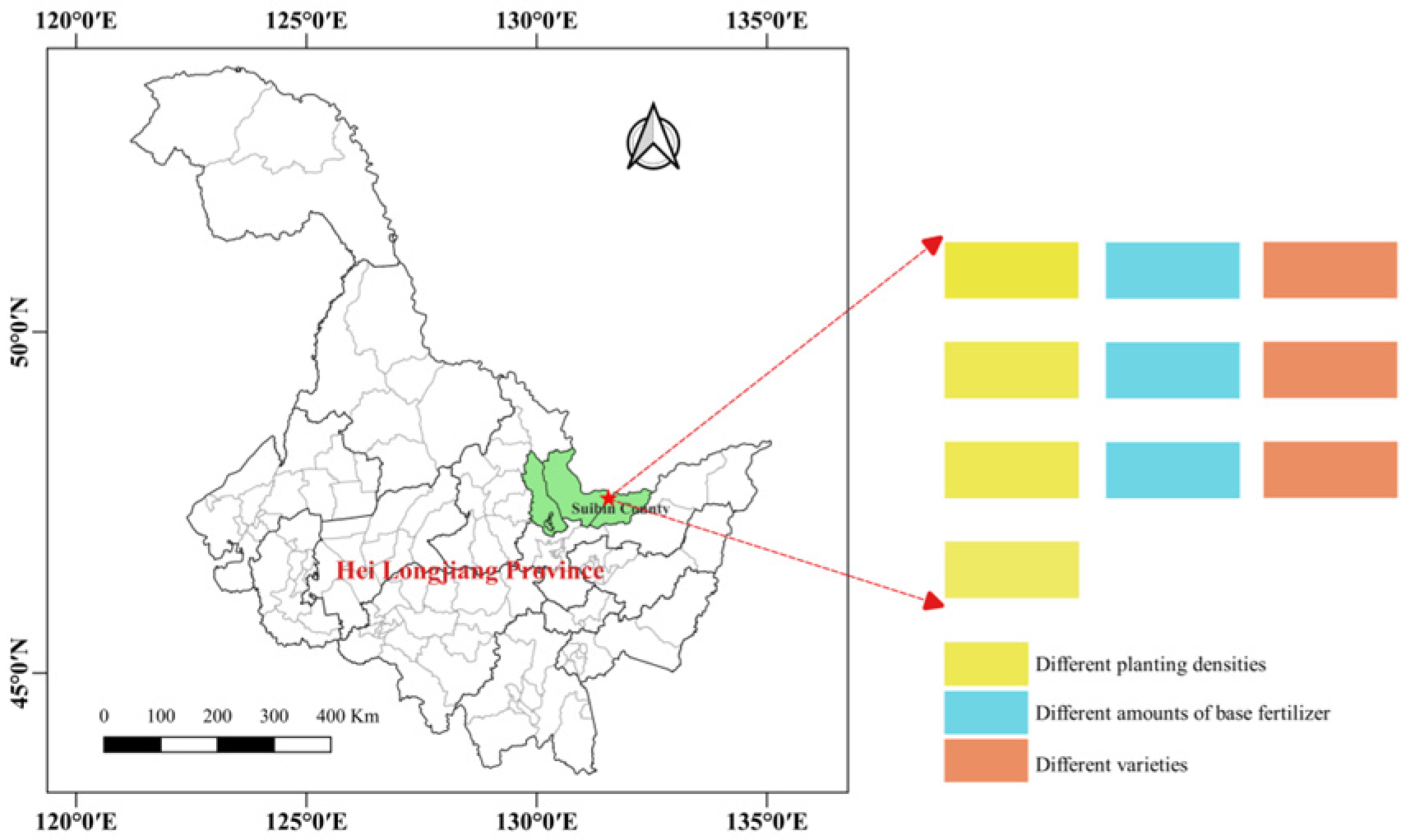
Figure 1. Location of the study area and experimental setup. There are 4 plots with different planting densities and 3 plots with different base fertilizer amounts and varieties, which correspond one-on-one with the information in Table 1.
Agronomy 14 01890 g001
Figure 2. Image acquisition equipment. (a) DJ M300RTK, UAV used in the experiment; (b) MS600 Pro, the multispectral camera installed; (c) Zenmuse P1, the RGB camera installed.
Agronomy 14 01890 g002
Figure 3. Calibration of the UAV calibration board.
Agronomy 14 01890 g003
Figure 4. Field sampling site for manual collection.
Agronomy 14 01890 g004
Figure 5. Framework for rice yield estimation. The framework consists of three parts, namely, data acquisition and preprocessing, data augmentation and model training, and model evaluation and validation.
Agronomy 14 01890 g005
Figure 6. Correlations of various multispectral VIs with yield. Red indicates a strong negative correlation and green indicates a strong positive correlation.
Agronomy 14 01890 g006
Figure 7. Correlation matrix diagram.
Agronomy 14 01890 g007
Figure 8. DNN architecture. Light green circles represent input features, while brown circles represent neurons in the hidden layer, where light brown represents neurons discarded by dropout and dark brown represents neurons preserved. The dark green circle represents the output.
Agronomy 14 01890 g008
Table 1. Information on experimental field plots.
PlotRice VarietiesPlanting Density (cm)Basal Fertilizer Amount (kg/ha)
1Songjing 53530 × 1225
2Suijing 18
3Kendao 94
4Longjing 3130 × 1226.25
527.5
628.75
7Longjing 3125 × 1225
825 × 14
930 × 10
1030 × 12
Table 2. MS600 Pro multispectral camera parameters.
ChannelChannel NameCenter Wavelength (nm)Spectral Bandwidth (nm)
1Blue45035
2Green55525
3Red66020
4Red edge 172010
5Red edge 275015
6Near Infrared84035
Table 3. Original data.
DatasetCategory I
Yield: 6000–8250 kg/ha
Category II
Yield: 8250–10,500 kg/ha
Category III
Yield: 10,500–12,750 kg/ha
Total
Original Data8014469293
Original Training Data6411555234
Original Test Data16291459
Table 4. VIs used in this study.
Serial NumberVIFormula
1CVI (Chlorophyll Vegetation Index) R n i r × R r e d / R g r e e n 2
2CI (Coloration Index) R r e d R b l u e R r e d
3GLI (Greater or Less Ratio Index) 2 × R g r e e n R r e d R b l u e 2 × R g r e e n + R r e d + R b l u e
4NGRDI (Normalized Green–Red Difference Index) R g r e e n R r e d R g r e e n + R r e d
5NDVIRE (Normalized Difference Vegetation Index Red edge) R n i r R r e d e d g e R n i r + R r e d e d g e
6RI (Redness Index) R r e d R g r e e n R r e d + R g r e e n
7GRVI (Green–Red Vegetation Index) R g r e e n R r e d R g r e e n + R r e d
8IO (Simple Ratio Red/Blue Iron Oxide) R r e d / R b l u e
9RGR (Red/Green Ratio Index) R r e d / R g r e e n
10MTCI (Modified Triangular Chlorophyll Index) R n i r R r e d e d g e R r e d e d g e R r e d
Table 5. Dataset after data augmentation.
DatasetData ComponentsNegative Samples IPositive SamplesNegative Samples IITotal
Training DataOriginal6411555234
Augmented48/57105
Test DataOriginal16291459
Augmented12/1426
TotalOriginal8014469293
Augmented60/71131
Original + Augmented140144140424
Table 6. Experimental modeling results without feature selection and data augmentation.
ModelR2RMSE (t/ha)
PLSR0.5141.07
SVR0.5031.08
RF0.5890.98
DNN0.6190.95
Table 7. Experimental modeling results without feature selection but with data augmentation.
ModelR2RMSE (t/ha)
PLSR0.6410.92
SVR0.6710.89
RF0.7520.74
DNN0.7700.73
Table 8. Experimental modeling results without data augmentation after feature selection.
ModelR2RMSE (t/ha)
PLSR0.5291.05
SVR0.5241.06
RF0.6080.96
DNN0.6340.93
Table 9. Experimental modeling results of feature selection and data augmentation.
ModelR2RMSE (t/ha)
PLSR0.6880.89
SVR0.7000.87
RF0.7820.73
DNN0.8100.69
Table 10. DNN results using the training and testing sets.
Feature Selection MethodData AugmentationTraining DataTest Data
R2RMSE (t/ha)R2RMSE (t/ha)
PearsonNo0.8330.650.6190.95
Yes0.8740.550.8100.69
Table 11. Results of yield estimation under different feature selection methods.
Feature Selection MethodData AugmentationR2RMSE (t/ha)
RFNo0.6270.94
Yes0.7970.74
PearsonNo0.6340.93
Yes0.8100.69
Disclaimer/Publisher’s Note: The statements, opinions and data contained in all publications are solely those of the individual author(s) and contributor(s) and not of MDPI and/or the editor(s). MDPI and/or the editor(s) disclaim responsibility for any injury to people or property resulting from any ideas, methods, instructions or products referred to in the content.