From Field to Model: Determining EROSION 3D Model Parameters for the Emerging Biomass Plant Silphium perfoliatum L. to Predict Effects on Water Erosion Processes

Abstract

The agricultural production of maize (Zea mays L.) increases the risk of water erosion. Perennial crops like cup plant (Silphium perfoliatum L.) offer a sustainable alternative to produce biomass for biogas plants. The assessment of soil conservation measures requires calibrated soil erosion models that spatially identify soil erosion processes. These support decision-making by farmers and policymakers. Input parameters for the physically based soil erosion model EROSION 3D for cup plant cultivation were established in a field study. Rainfall simulation experiments were conducted to determine the model input parameter’s skinfactor and surface roughness. The results showed a reduction of soil erosion and higher infiltration rates for cup plant resulting in higher skinfactors of 11.5 in June and 0.75 post-harvest (cup plant) compared to 1.2 in June and 0.21 post-harvest (maize). With the extended parameter catalogue of EROSION 3D for cup plant cultivation model simulations were conducted for a rainfall event in June (64 mm). The sediment budget would have been reduced by 92.6% through the growth of cup plant in comparison to conventionally grown maize. Perennial cup plant can, therefore, contribute to achieving the targets outlined in the European Green Deal by reducing soil erosion and enhancing soil health.

1. Introduction

The European Green Deal represents a comprehensive strategy to combat climate change and environmental challenges, with soil protection playing a central role in achieving sustainable development goals by 2030 [1,2]. Minimizing soil erosion is one of ten of the FAO-defined voluntary guidelines for sustainable soil management and was endorsed by all FAO Members, including the EU Member States [1,3]. Agriculture, as the largest land user of the European Union, plays a vital role in achieving these goals, including the production of biomass for renewable energy plants [4]. In Germany, the commitment to increasing the share of renewable energies to 80% by 2030, as legislated by the German Renewable Energy Act [5], underscores the nation’s dedication to sustainable energy practices. In 2020, energy crops for biogas production were cultivated on approximately 1.5 million hectares of arable land in Germany [6]. The proportion of maize (Zea mays L.) in this area is around 65% [6]. Maize exhibits high water-use efficiency, established cultivation methods, and provides substantial biogas yields [7]. However, annual row crops have led to a series of environmental concerns due to loss of biodiversity or land degradation through soil erosion [8]. In particular, maize cultivation on slopes increases the risk of water erosion [9,10]. A study conducted in a low mountain range region in Western Germany found that about 30% of maize is grown on fields with high soil erosion potential, and about 10% of maize is cultivated on fields with an increased risk of soil compaction [11]. Soil and nutrient losses due to water erosion can result in surface water eutrophication and the loss of fertile soil for crop production. Predicted climate change scenarios further aggravate the risk of water erosion. Higher winter precipitation and more frequent extreme summer precipitation raise concerns regarding conventional cultivation on slopes or soils with low water infiltration capacity [12,13,14]. Soil cover during these vulnerable periods is crucial for soil erosion prevention [15].

The anticipated increase in soil erosion on arable land poses a threat to food supply and human well-being [16,17] and widely exceeds the rates of soil formation [18]. Soil erosion can cause high ecological and economic costs [19,20]. In addition to water eutrophication, other ecological consequences encompass the loss of soil organic carbon, intensifying global warming [21]. However, by fostering sustainable agricultural practices, it is also recognized that soils can be a significant component in fulfilling the objectives of the European Green Deal [22].

In order to increase sustainable biomass production, stakeholders develop various strategies to reduce water erosion. On the one hand, technical solutions like strip-till, mulching, intercropping, direct seeding, or contour seeding are implemented. On the other hand, the cultivation of crops that are less prone to soil erosion is discussed, with perennial crops being of particular interest [23,24]. The advantage of perennial crops is that soil tillage will only be conducted during the establishment of the crop. Root systems of such crops remain undisturbed afterward. It could be demonstrated that perennial crops present promising solutions to reduce soil erosion and nutrient losses and can protect surface water bodies from sediment and nutrient loads [25,26,27,28,29]. Cup plant(Silphium perfoliatum L.) emerge as a promising bioenergy crop among these alternatives. Next to high biomass yield, cup plant provide additional ecological benefits, e.g., soil protection and pollinator support [30,31,32]. Thus, cup plant add more diversity to rural areas than most common annual crops [33], addressing more than one of the environmental challenges defined by the EU and FAO [1,3]. Cup plant have the potential for high biomass yield on soils with high water availability, albeit with lower methane yields than silage maize [7,34]. It has been shown that cup plant can be harvested for at least ten years with minimal pesticide use [30]. Cup plant harvest takes place once a year between late August and September, after which cup plant continue to grow, acting as a catch crop and positively affecting soil fauna [35,36,37]. Therefore, the potential to reduce soil erosion by cup plant should be quantified in a field study.

Erosion models have been used for decades to assess erosion risk on arable land, providing a systematic basis for soil erosion estimates [38,39]. For example, Wang et al. [28] demonstrated with a modeling study on switch grass that strategic placement of perennial bioenergy crops in the field or watershed can have a positive ecological impact. A reduction of soil erosion while providing the required feedstock for the biofuel industry was calculated [28]. The commonly assumed notion that small areas of a field (hotspot areas) contribute predominantly to the overall soil erosion was supported by a time-series soil erosion model analysis by Höfler et al. [40].

Soil erosion models can be classified into empirical, physically based, or conceptual models, which describe and formalize the influence of soil, climate, land cover, topography, and vegetation parameters on soil erosion risk [41]. Physically based models, such as the EROSION 3D model [42], have gained prominence since these describe the phases of the erosion process mathematically, taking into account the fundamental concepts of physics [43]. Thus, these models consist of multiple algorithms and a large number of parameters to predict the dynamics of soil erosion [41]. Physically based models have great explanatory power, but their predictive accuracy depends on calibrating the input parameters [44].

The EROSION 3D model, employed in several federal states in Germany, is used to assess the soil erosion risk on arable land and to develop mitigation strategies for sustainable agricultural landscapes [45]. It operates on an event-oriented basis and has also been used to evaluate the erosion mitigation potential of future cropping system designs [46]. Vogel et al. [9] used Erosion 3D to design various field layouts to reduce erosion in bioenergy crop production, integrating strategies such as buffer strips and vegetated waterways. EROSION 3D needs, besides rainfall and topographic data, a further eight soil parameters [42]. Five soil parameters can be acquired with standard methods of soil analyses or estimated from soil maps [47]. The other three soil parameters (surface roughness, resistance to erosion, and skinfactor) can be determined from rainfall simulator experiments or estimated based on an existing parameter catalogue of EROSION 3D. This allows the application of EROSION 3D with moderate calibration effort [47]. The model has undergone international validation [48,49,50,51,52,53,54,55,56,57,58,59] and has been utilized in numerous international soil erosion studies [46,47,50,51].

However, the model’s parameter catalogue (mean calibrated input parameters) of EROSION 3D relies on findings from heavy rainfall simulations conducted under field conditions, primarily during the mid-1990s [52]. The parameter catalogue was supplemented by the results of a study applying a small-scale rainfall simulator by Schindewolf and Schmidt [53]. Updating the model’s parameter catalogue is necessary to adapt EROSION 3D for evolving agricultural practices. For example, introducing perennial crops like cup plant or changes in direct seeding techniques like strip-till requires the extension of the parameter catalogue. Additionally, climate change’s effects on soil erosion must be considered [15].

Therefore, the main aim of this study is to determine the input parameters that are lacking for the EROSION 3D model for cup plant cultivation. Rainfall simulation experiments were used to calibrate the model input parameters for the skinfactor and surface roughness of cup plant. These parameters were validated with recorded data of natural precipitation events of a field trial, as a control of the used methods and to compare parameters obtained for maize from this field trial with parameters provided by the parameter catalogue of EROSION 3D. These newly calibrated input parameters for cup plant were used to demonstrate the potential reduction of soil erosion by the calculation of erosion scenarios for different agricultural management practices. Farmers and decision-makers will be able to model the effects of cup plant cultivation in comparison to annual row crops with EROSION 3D. Successful implementation of input parameters for cup plant can support farmers’ decision-making process toward more sustainable perennial biomass production in the future.

2. Materials and Methods

2.1. Site Characteristics and Site Management

The presented study is based on a field experiment, which was established in the low mountain area at Elm Mountain close to Erkerode, Germany (52.203019° N, 10.714348° E) in spring 2021. The experimental site has a 13% northwest exposed slope (Figure 1(1)).

The soil at the field was classified as a Luvisol, according to the World Reference Base for Soil Resources [54]. The soil texture was characterized by 13% sand, 70% silt, and 17% clay in 0–30 cm topsoil and did not vary much up to 90 cm depth. The soil had an organic carbon content of 1.1% at 0–30 cm depth. The soil bulk density ranged from 1.42 g/cm³ in 3–8 cm depth to 1.62 g/cm³ in 30 cm depth. The annual precipitation was 711 mm, and the average daily temperature was 9.1 °C (1991–2020) [55]. The main focus of the experiment was to quantify soil erosion of cup plant, conventionally grown maize (annual plowing to a depth of 25 cm and seedbed preparation with a rotary harrow) and maize directly seeded (no-tillage) in a completely randomized block experiment with three replicates (Figure 1(1)). The resulting nine plots were placed along the slope with an erosive slope length of 45 m. All plots were 6 m wide. Crops were drilled in the slope’s direction. Rainfall data during the research period were collected using an automated weather station (Vantage Pro2, Davis Instruments, Hayward, CA, USA) installed close to the experimental plots (Figure 1(1)).

Each rainfall event was characterized by the maximum rainfall intensity in 30 min (I30) and rainfall erosivity (EI30) calculated according to the algorithms given in DIN 19708:2017-08 [56]. Soil cover was measured weekly across all plots. Three photos were taken per plot at three locations and analyzed using image processing software by Riegler-Nurscher et al. [57]. The field experiment aimed to (1) quantify the erosion mitigation potential of cup plant in comparison to maize on slopes and (2) determine the necessary input parameters for the physically based soil erosion model EROSION 3D for cup plant. The latter was the subject of the present study, which started in the spring of 2022 after the cup plant was established in 2021.

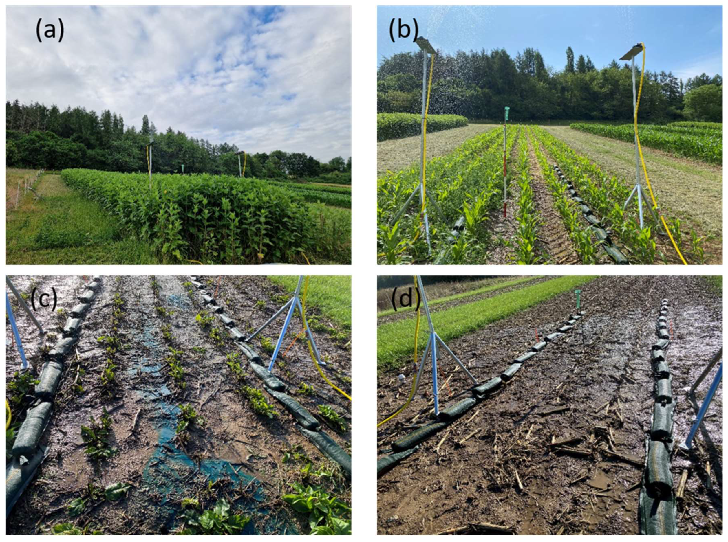
2.2. Rainfall Simulator Experiment for Model Calibration

Heavy rainfall was simulated to calibrate specific EROSION 3D model input parameters [42,52,53] for cup plant in September 2022 and June 2023. For the validation process (Section 2.6), rainfall simulations were also conducted on the conventionally tilled and no-till maize plots. The rainfall simulation experiments were conducted on subplots of 12.5 m² size (2.5 m width × 5 m length) at the lower end of the main plots of Block 1 of the experimental field (Figure 1(1); one plot per treatment). A rainfall simulator was designed based on Nielsen et al. [58]. The rainfall simulator (Figure 2) was modified in such a way that the water stream was directed upwards so that drops were formed (semi-)gravitationally and achieved terminal velocity through free fall. The rainfall simulator consisted of two rainfall modules, allowing the irrigation of the subplot from both sites. Four main components can be distinguished:

• an automated sprinkler to generate and distribute water droplets;
• a tripod to elevate the sprinkler with an adjustable height of up to 3 m;
• a pump to supply the system with water from a tank;
• a water tank supplying the system with water.

The sprinkler was a commercially available Gardena Aquazoom^® oscillation sprinkler (Gardena Deutschland GmbH, Ulm, Germany) that formed a one-dimensional arc boom. In order to counteract the oscillating effect and, thus, an interruption of the irrigation on the plot, two oscillating sprinklers with opposite oscillation cycles were placed opposite each other. Nielsen et al. [58] elaborated on drop size distribution (DSD) and applied kinetic energy of the Gardena Aquazoom^® sprinkler (kinetic energy of 34.9 J m⁻² mm¹ for one sprinkler). A water pump (Cleancraft FWP 50, Stuermer Maschinen GmbH, Hallstadt, Germany) was used for constant water supply from an 8000 L mobile water tank. Rainfall intensity and spatial rainfall distribution for this study were calibrated during the construction phase of the rainfall simulator. A target rainfall intensity of 60 mm/h and uniformity of at least 80% was calibrated. The rainfall intensity was measured via a rain gauge, and spatial uniformity was elaborated on using the Christiansen coefficient of uniformity (CU) [59]. The calibration procedure was conducted as described by Koch et al. [60] and falls 80% in the range of other European rainfall simulators [61]. Prior to each rainfall simulation, soil water content at 0–15 and 15–30 cm depth was measured gravimetrically near the subplot (n = 5).

During the rainfall simulation, constant rainfall was applied to soil with natural moisture conditions. Due to uncontrollable effects, the rainfall intensity may vary slightly. To determine the actual rainfall intensity, a rain gauge (TFA 47.1013, TFA Dostmann GmbH & Co. KG, Wertheim-Reichholzheim, Germany) was installed in the plot area (Figure 2b). Runoff was measured continually via the soil erosion measurement system (SEMS; see Section 2.3) until nearly constant runoff occurred. Runoff sampling was conducted every five minutes to measure sediment concentration [62]. Runoff velocity of each treatment was measured by adding brilliant blue (Brilliantblau FCF EG-Nr. 233-339-8, Carl Roth GmbH & Co. KG, Karlsruhe, Germany) as a tracer to the runoff at the top of the slope when constant runoff was reached at the end of the rainfall simulation. The time the tracer needed from the top to the bottom of the slope was used to calculate surface roughness according to Manning’ equation (Equation (2)).

Rainfall simulations were carried out in September 2022 and June 2023 under typically high-risking conditions for water erosion in crop production. In September, most summer crops have been harvested, leaving bare soil prone to erosion. Contrary to these, cup plant stands are characterized by regrowth after harvest and a permanent living root system. All treatments (maize and cup plant) were mulched after harvest in September 2022, three weeks before the rainfall simulation took place. In June, low soil cover of late-sown summer crops and high rain erosivity are critical factors contributing to erosion processes [9,12,13,15]. Other than late-sown summer crops, cup plant covered the soil to 90% in June, preventing direct splash erosion.

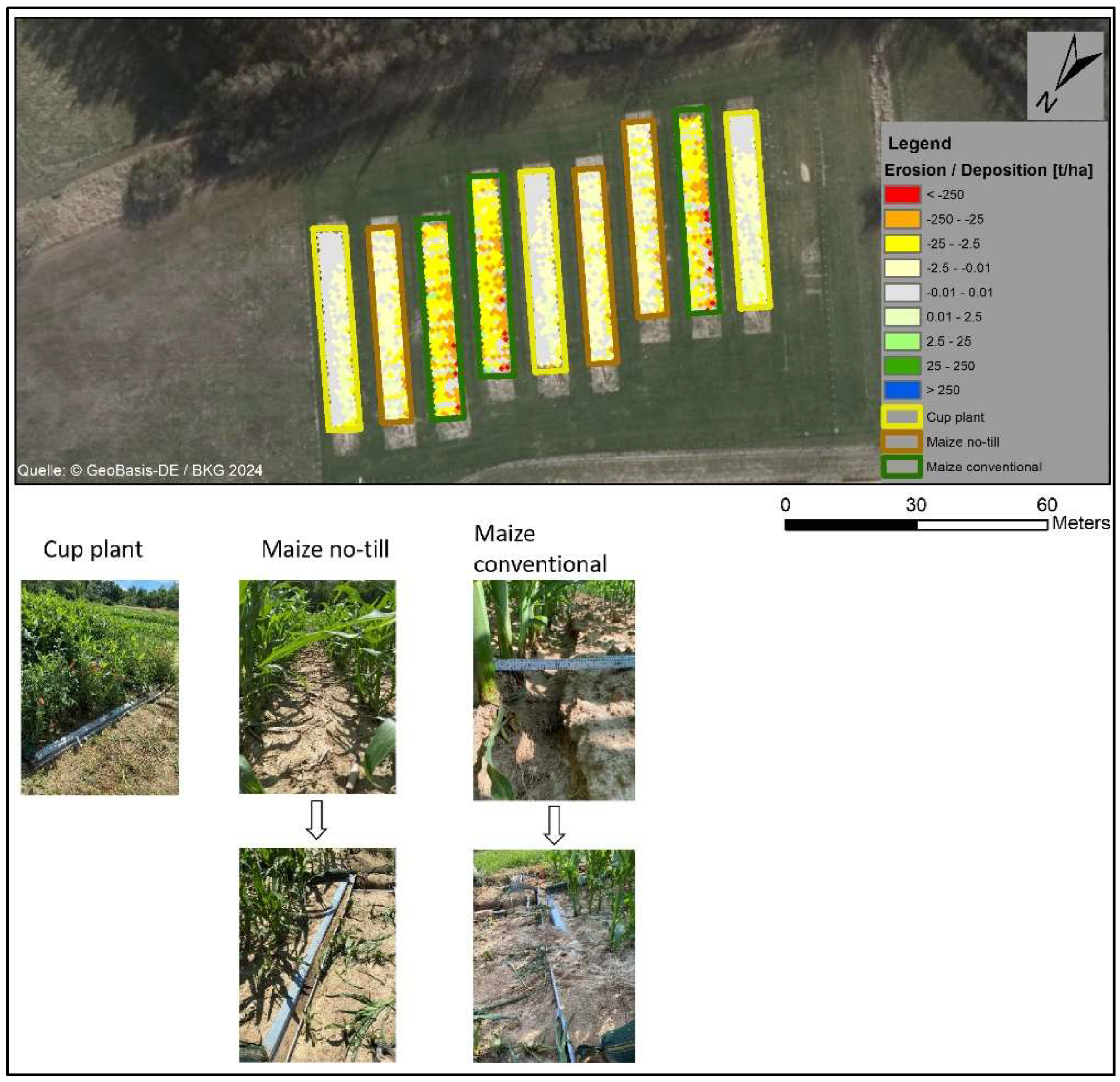
2.3. Natural Runoff and Soil Erosion Measurement

Runoff and soil erosion were measured for a partition of each plot during natural precipitation events. The hillslope length multiplied by the width of the SEMS of 2.5 m inside the 6 m wide plots (Figure 1(2a)) contributed to the SEMs of each plot. Three crop rows (row width 0.75 m) were covered by the 2.5 m, including one single traffic line. Customized SEMSs collected runoff and suspended soil in a flume in case of erosive events and routed the suspension into tipping buckets (UP GmbH, Ibbenbueren, Germany). A proportional sample of this suspension was collected for further analysis. In detail, the flume system consisted of an inflow metal sheet overlapping the PVC flume (3 m PVC flume with bypass and weir at 2.5 m) (Figure 1(2b)) with an open outlet to a modified Gerlach trough [63]. To ensure that runoff and sediment from the plot area flowed into the flume system, inflow metal sheets were installed at the bottom end of the plot (Figure 1(2b)). Figure 1(2c) shows the profile view of the inflow of metal sheets into the soil. The inflow metal sheets provided a vertical drop at the boundary between the slope and the flume at the bottom end of the plot. The flume was orthogonally installed to the slope gradient. A weir ensured the flow through the bypass up to a flow rate of 30 L/min. In cases of rain events resulting in more than 30 L surface runoff per minute towards the PVC flume, the runoff suspension overflowed the weir behind the bypass further down the flume to the modified Gerlach troughs (Figure 1(2a)). The amount of eroded soil material settling in the flume was quantified after rain events. In case of overflows, soil particles settled in the modified Gerlach troughs were recovered and quantified. The size of the flume and Gerlach trough determined the maximum soil loss to be quantified.

Before installing the tipping buckets in the field, each tipping bucket was calibrated on the tipping rate and tipping volume (1800 L/h with an error of 0.03%). The tipping buckets were customized with a sampling divider (UP GmbH, Ibbenbueren, Germany); about 1% of each tip (one tip is 1 L) was diverted to a sampling bottle. The sampling bottles were emptied after each erosion event, and samples were taken to the lab for further analysis. The suspended sediments were separated from runoff by filtration (Grade 132, Sartorius AG, Göttingen, Germany), and the sediments were oven-dried at 40 °C. The sediment concentration of the runoff of the plot was calculated by multiplying the weight of oven-dried sediment samples with the total volume of runoff suspension and this was added to the settled sediments in the flume system.

2.4. Model Background

EROSION 3D (Version 3.3.2.0, Geognostics, Berlin, Germany) was developed as a physically based soil erosion model that calculates soil particles’ detachment, transport, and deposition initiated by single-rainfall events or event sequences in small watersheds [42,64].

EROSION 3D uses a momentum flux-based model approach in which particle detachment occurs when the combined momentum flux of surface runoff and raindrop impact exceeds soil-specific erosion resistance [42]. To characterize the soil’s resistance to erosion, the model expresses the critical momentum flux φ_crit according to:

φ_crit = (q_crit × p_q × v_q)/∆x

(1)

where q_crit is the volume rate of flow (m³/(m × s)) at initial erosion, which depends on soil texture, organic carbon, tillage, etc.; p_q is the fluid density (kg/m³), ∆x is the slope segment (m), and v_q is the flow velocity according to Manning’s equation:

v_q = 1/n × δ^2/3 × S^1/2

(2)

where n is the roughness coefficient (s/m^1/3), δ is the layer thickness of runoff (m), and S is the slope inclination (%).

Infiltration is calculated according to a modified Green and Ampt approach, which assumes a rigid soil matrix [42]. Temporal soil structure changes caused by, e.g., tillage or biological activities are considered by the empirical parameter skinfactor [42,53]. The skinfactor allows the calibration of saturated hydraulic conductivity through soil- and management-specific infiltration experiments [54]. This is defined as:

k_s = k_sat × skin

(3)

where k_s is saturated hydraulic conductivity adjusted by skinfactor (kg × s/m³), k_sat is saturated hydraulic conductivity (kg × s/m³), as calculated by Campbell [65]; and skin is skinfactor (−).

Hence, values of skinfactor < 1 reduce the simulated infiltration rate in order to take the effects of soil slaking and sealing, as well as the soil compaction, into account. Values of skinfactor > 1 cause a positive correction of infiltration rate to consider increased infiltration due to, e.g., tillage impact [53].

After the detachment process, soil particles were transported in suspension. The deposition was calculated using hydraulic conductivity and Stokes law, respectively. As a grid-based model, slope angle and aspect were determined for each grid element. Flow distribution was calculated using either the D8 algorithm, which directs runoff to the lowest grid neighbor, or the FD8 algorithm, which proportionally distributes runoff to all lower grid neighbors based on the altitude difference [64]. For sheet flow conditions, the FD8 algorithm exhibited superior and more natural flow distribution compared to the D8 algorithm [66] and was chosen in this study. A detailed description of the modeling algorithm and main equations implemented in the model can be found in Schmidt et al. [42]. EROSION 3D was initially calibrated and validated through 116 rainfall simulation studies on agricultural fields in Saxony, Germany, conducted from 1992 to 1996 [52].

2.5. Determining Input Parameters from Experimental Data

In order to determine the model-specific parameter skinfactor, the R package toolbox E3D (Available online: https://github.com/jonaslenz/toolbox.e3d (accessed on 6 September 2024)) [67], and EROSION 3D (Version 3.3.2.0, Geognostics, Berlin, Germany) was used. All parameters are listed in

Table 1. EROSION 3D model input parameters.

Input Parameter	Unit	Data Source
Altitude DEM	(m)	Digital elevation model with a resolution of 1 m (Landesamt für Geoinformation und Landesvermessung Niedersachsen LGLN © 2024)
Soil cover	%	Field measurement
Bulk density	kg/m3	Field measurement according to DIN ISO 11272 (available online: https://www.dinmedia.de/de/norm/din-en-iso-11272/263368180 (accessed 2 September 2024))
Soil organic carbon content	%	Field measurement according to DIN ISO 10694 (available online: https://www.dinmedia.de/de/norm/din-iso-10694/2799936 (accessed 2 September 2024))
Grain size distribution	%	Field measurement according to DIN ISO 11277 (available online: https://www.dinmedia.de/de/norm/din-iso-11277/53934894 (accessed 2 September 2024))
Skinfactor	-	Rainfall experiment
Surface roughness	s/m1/3	Rainfall experiment
Initial soil moisture *	%	Field measurement/Parameter catalogue EROSION 3D
Erosion resistance	N/m2	Parameter catalogue EROSION 3D
Rainfall intensity	mm/min	Field measurement (rain gauge)

* For model validation and model application’s initial soil moisture data were derived from the parameter catalogue EROSION 3D.

. The skinfactor was iteratively adjusted to the amount of cumulative runoff from the plot area [52]. The erosion rates calculated with EROSION 3D depend on the transport capacity of the surface runoff, which in turn is influenced by the slope length (Equation (1); [53]). Slope lengths ranging from 20 to 150 m most commonly achieve maximal transport capacity [53]. Consequently, the plot length in our rainfall simulation experiment was not sufficient to ensure adequate surface runoff for maximal transport capacity rates. As a result, this study did not calculate the resistance to erosion factor; instead, this factor was derived using the parameter catalogue of EROSION 3D.

2.6. Validation of the Model Performance

The experimentally obtained input parameters for EROSION 3D were validated using field observations. Single storm simulations were conducted using natural rainfall data measured during the summer of 2022 (

Table 2. Observed natural rainfall characteristics at the study site were used to validate the parameterized model EROSION 3D.

Erosion Event	Date	Rainfall Erosivity * (EI30, N/h−1)	Rainfall Intensity (I30, mm/h)	Duration (min)	Rainfall (mm)	Soil Cover (%)
						Cup Plant	Maize No-Till	Maize Conv.
E1	24 June 2022	180.0	124.8	260	64.6	95	66	70
E2	8 September 2022	8.2	15.2	405	27.6	5	5	5

* Rainfall erosivity, a measure of soil erosion potential, is the ability of rain to cause erosion. It depends on the amount and intensity of rain [68].

). The results of the simulations were compared to erosion measurements in the field. Due to the spatial resolution of the pixels and the chosen FD8 algorithm, the sum of two pixels at the bottom of the plot was selected to compare the modeled results with observed values.

The measured precipitation events can be classified according to the recurrence interval, i.e., the average period of time in which an event reaches or exceeds a value once. This was done using the KOSTRA data set provided by the German Weather Service (DWD; available online: https://www.openko.de/kostra-dwd-2020-rasterfeld-nr-113153/ (accessed on 6 September 2024)). The exceptional heavy rainfall event E1 exceeded the threshold value for a 100-year event at this location, with an erosivity value of 180 N/h⁻¹. In North-Eastern Germany, a 100–year event is characterized by an erosivity value of 71 N/h⁻¹ [12]. The second event E2 had a probability of recurrence of two years.

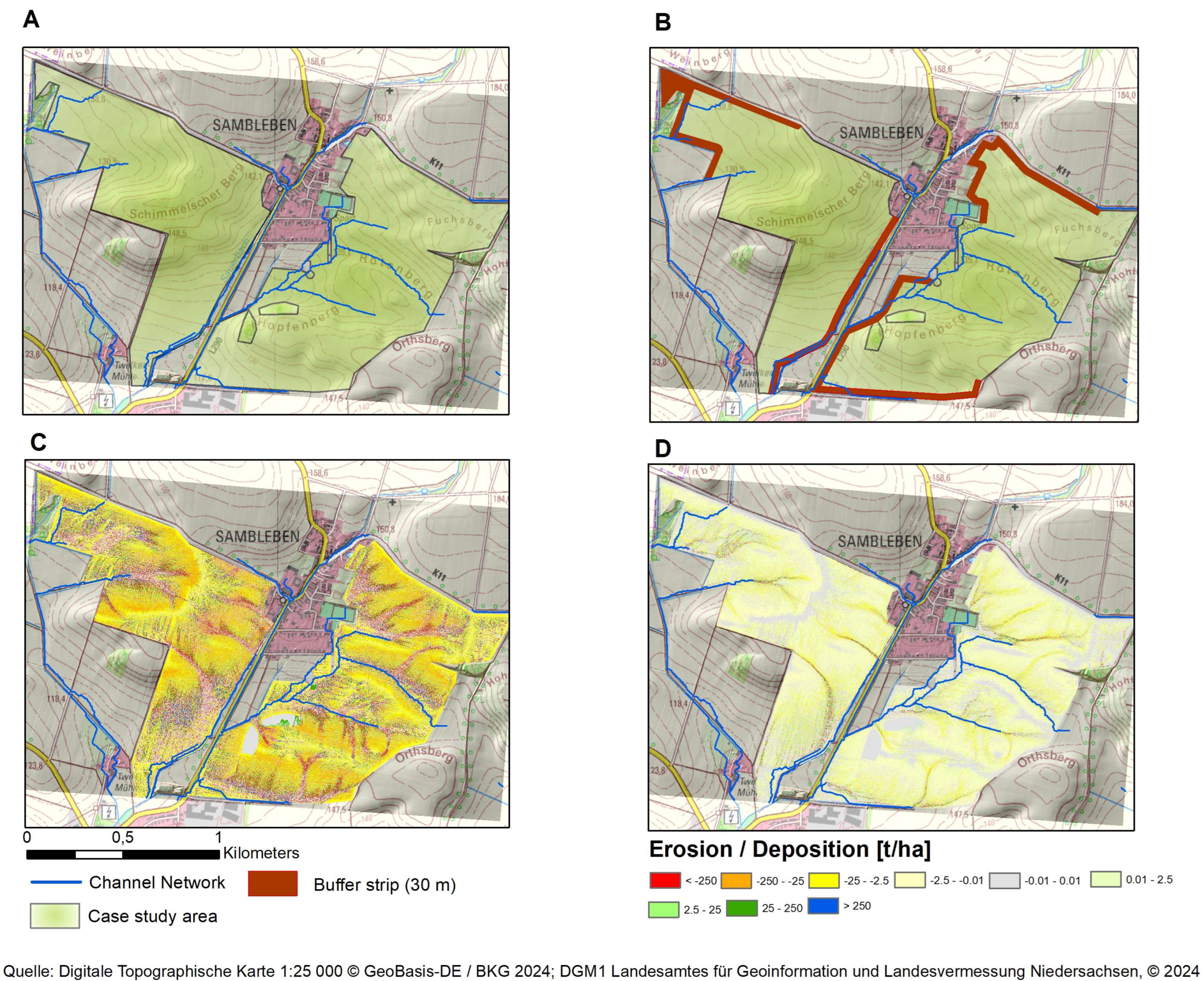
2.7. Model Simulation to Explore Management Effects on Soil Erosion Using Experimentally Determined Parameters

Using the calibrated parameters, EROSION 3D was applied in a case study to demonstrate the potential reduction of soil loss through water erosion. For this application of the model, field blocks close to the experimental field at Elm Mountain were chosen. Soil data were assumed to be similar to the soil data of the experimental field (Section 2.1). A recorded rainfall event in June 2022 (E1) with a total of 64 mm rainfall in 260 min and an erosivity of 180 N/h was used in time steps of 5 min for the simulation. Five scenarios were modeled:

• The first “worst case” scenario represents conventional maize cultivation across the entire field. This scenario serves as a baseline for comparison, reflecting typical farming practices for bioenergy cropping.
• In the second scenario, maize would be cultivated without tillage (no-till).
• In a third scenario, established cup plant stands would grow on the test sites.
• The fourth scenario combines conventional maize cultivation with a buffer strip (30 m width) cultivated with cup plant for water retention and soil protection.
• Lastly, the fifth scenario combines no-till maize with the same buffer strip.

3. Results

The presented results were divided into three sections. First, the experimental parameterization of skinfactor and surface roughness of cup plant. Second, the evaluation of the performance of the model. Third, the presentation of erosion scenarios.

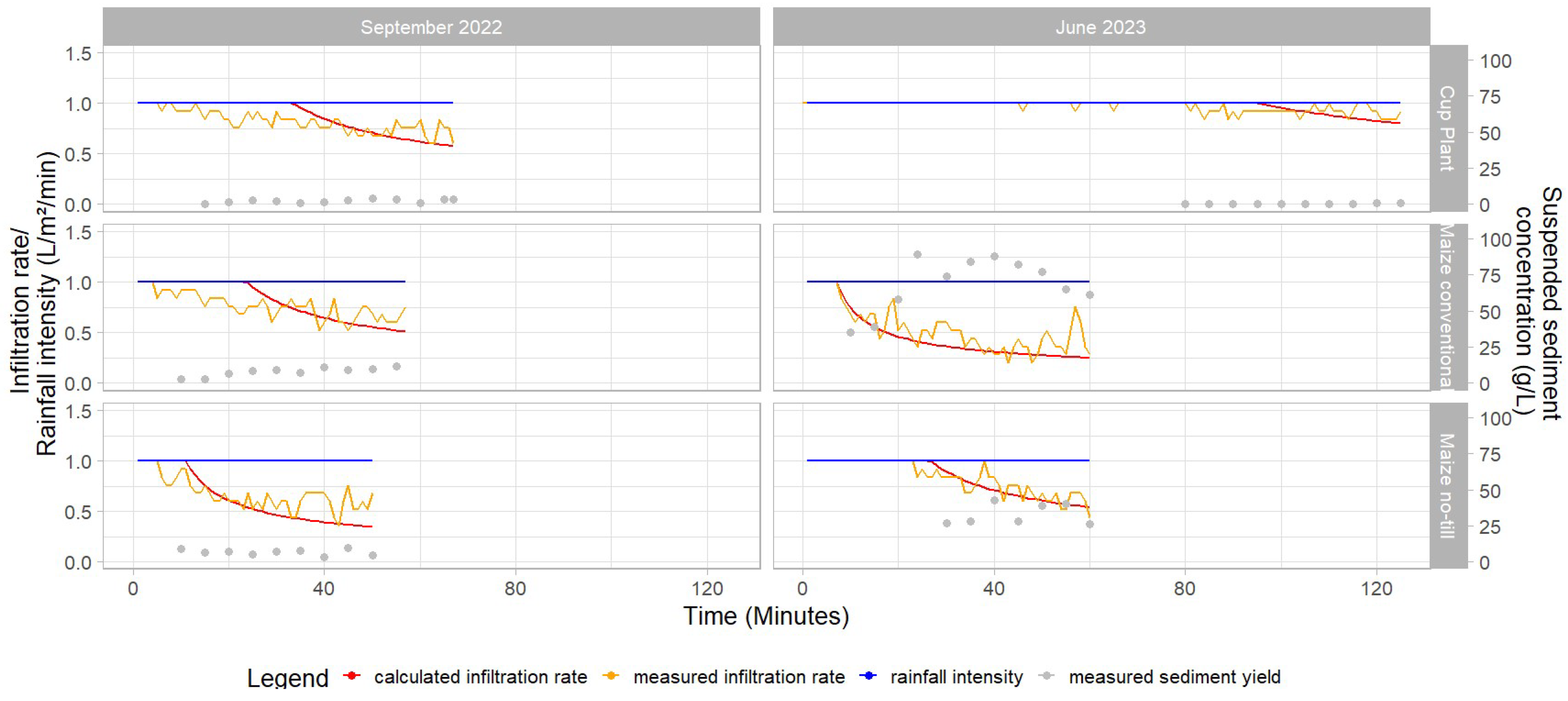
3.1. Rainfall Simulation for Model Calibration

Table 3. Calibrated skinfactor and surface roughness values were calculated for the rainfall simulation experiments in September 2022 and June 2023.

	September 2022 *		June 2023
Treatment	Skinfactor (-)	Surface Roughness (s/m1/3)	Skinfactor (-)	Surface Roughness (s/m1/3)
Cup plant	0.72	0.431495	11.5	0.491129
Maize conv.	0.16	0.144314	1.2	0.091000
Maize no-till	0.21	0.319425	3.6	0.120144

* Stubble of all treatments were mulched post-harvest.

shows skinfactors gained through the simulated rainfall experiments. Cup plant resulted in significantly higher skinfactors than both maize tillage practices, which was expected. No-till maize resulted in higher skinfactors than conventionally tilled maize, indicating more macro pores open to the soil surface and less soil sealing (Table 3). In September 2022, after harvesting and mulching all three treatments, the re-growth of cup plant and the living rooting systems resulted in a 3–4 times higher skinfactor than the maize treatments. An even more pronounced difference between conventionally tilled maize and cup plant cultivation could be observed in June 2023, when the skinfactor was ten times higher. Replacing conventional tillage with a no-till soil management increased the skinfactor three times in June.

Figure 3 compares the calculated infiltration rate from EROSION 3D with measured infiltration rates during rainfall simulations in September 2022 and June 2023 for all three treatments. It can be seen that on the conventionally tilled maize plots, in contrast to the cup plant and no-till maize plots, infiltration decreased substantially over time and eventually leveled off, especially in June. High infiltration rates were recorded for the cup plant from the rainfall simulation’s start, decreasing only slightly over time. Infiltration rates of no-till maize were higher than of conventionally seeded maize. The sediment concentration of the runoff suspension also varied substantially between the three treatments (Figure 3). While the cup plant exhibited very low sediment concentrations in both rainfall simulation experiments, the maize treatments differed considerably, especially in June. The conventional maize treatment had a higher and earlier onset of soil erosion, whereas the no-till treatment showed soil erosion later and to a lesser extent (Figure 3).

Experimentally assessed surface roughness values are presented for the different treatments for both dates of rainfall simulations in Table 3. Surface roughness increased from conventionally tilled maize to no-till maize and further to cup plant at both times, with the highest surface roughness values for cup plant in June 2023.

With the calibrated values for skinfactor and surface roughness, the study’s main aim was achieved. To increase the confidence in these values, records of natural precipitation events were used for validation in the next step.

3.2. Natural Precipitation Events for Model Validation

The validation of the model parameters for the cup plant used data from two natural rainfall events occurring during the study period (Table 2).

Table 4. Observed and modeled (EROSION 3D) runoff and sediment yield for cup plant. E1 = natural precipitation event in June 2022; E2 = natural precipitation event in September 2022.

		E1		E2
Crop	Replication	(Runoff (L); Sediment (kg))
		Observed	Modeled	Observed	Modeled
	1	(455; - *)	(580; 0.2)	(15; 0)	(17; 0)
Cup plant	2	(413; - *)	(488; 0.3)	(18; 0.012)	(16; 0)
	3	(-; - *)	(1280; 5.1)	(16; 0.028)	(15; 0)

* SEMS failed to record data; we were not able to measure the amount of sediment loss in runoff suspension because all the water samples were lost due to the severity of the event.

presents the comparison of observed and modeled runoff and soil loss for cup plant for all experimental plot replications and two natural rainfall events (E1 and E2).

The model accurately predicted runoff and soil loss for the E2 event, closely matching the observed measurements. However, discrepancies between the model predictions and observations were evident for the E1 event. Notably, the measuring system in replication three broke down during this exceptional heavy rainfall event E1, affecting the data collection process. All SEMSs of the maize plots failed to produce reliable data during the event E1 as well.

Visual inspections of the SEMS after the June event (E1) reflected the modeled erosion maps by EROSION 3D (Figure 4). Experimentally calculated skinfactor and surface roughness parameters were used (Table 3). Distinct signs of erosion were evident in the maize plots conventionally plowed. Figure 4 compares the erosion maps of all three treatments with the visually observed erosion in the experimental field after event E1. Notably, dark red-colored pixels are modeled only in maize plots conventionally plowed. These plots recorded erosion rills up to 20 cm wide and 3–5 cm deep.

3.3. Case Study on the Application of Cup Plant Parameters to Model Cultivation Strategies and Their Impact on Soil Erosion

Table 5. Statistical parameters of sediment budget per pixel cell for each scenario. A recorded rainfall event in June 2022 (Event 1, Table 2 with a total of 64 mm rainfall in 260 min) was used for model simulation.

Scenario	Sediment Budget per Pixel Cell (kg/m2)
	Median	Mean	Standard Deviation	Erosion Reduction (%)
Maize conv.	−0.4	−10.5	68.2	-
Maize no-till	0.0	−5.1	153.7	51.6
Cup plant	0.0	−0.7	23.6	92.6
Maize conv. + buffer strip cup plant	−0.2	−9.5	68.8	9.7
Maize no-till + buffer strip cup plant	0.0	−4.4	131.2	58.3

presents the main statistical parameters for each simulated scenario and the difference in mean sediment budget per pixel cell (1 × 1 m) between each scenario. Cup plant cultivation exhibited the most substantial decrease in mean erosion values, with a reduction of about 93% in comparison to the conventional maize scenario. Additionally, the no-till maize scenario demonstrated a decrease in mean erosion values, with a reduction of about 52%. Introducing buffer strips (Figure 5B) of cup plant into the conventional maize scenario reduced erosion by 9.7%. Adding buffer strips of cup plant to the no-till maize scenario reduced the erosion further by 6.7%. For a detailed examination of the impact of cup plant cultivation, the sediment budgets for conventional maize and cup plant scenarios were illustrated in Figure 5C,D.

4. Discussion

The primary objective of this study was to determine the necessary input parameters for EROSION 3D for cup plant, an emerging bioenergy crop. Exceptional characteristics of cup plant cultivation are the early canopy closure in spring and the regrowth after harvest [37]. Climate change is altering precipitation patterns and intensity, increasing erosion potential in spring and autumn [14,15,69,70]. Consequently, the total erosion potential is expected to change depending on whether bare soil between two consecutive crops occurs in the winter half-year (e.g., winter crops) or in the summer half-year (e.g., root crops). Strategically placed perennial biomass crops have the potential to reduce erosion. This emphasizes the importance of well-parameterized, physically based erosion models, such as EROSION 3D, as a tool for decision-making.

4.1. Rainfall Simulation for Skinfactor Calibration

Previous rainfall experiments by Grunwald et al. [27] demonstrated a notable reduction in runoff and soil erosion associated with cup plant cultivation. Likewise, infiltration measurements by Grunwald et al. [27] at the beginning of the vegetation period resulted in high infiltration rates of cup plant (1.9–5.0 mm/min). These were attributed to higher abundances or activity of earthworms [71,72,73], root systems, and litter [37]. Our rainfall experiments, particularly those conducted in June (Figure 3), corroborate these findings as we could not force erosion processes with a 1 mm/min rainfall intensity. High water retention (interception) and infiltration rates of cup plant led to near-zero runoff and soil erosion, while under conventional maize, high runoff and soil erosion were observed (Figure 3). In addition to the reported high number of earthworms in soils under cup plant, Wöhl et al. [37] discussed that ground cover, like litter layers, can considerably increase infiltration and decrease erosion in cup plant cultivation. Particularly during the early stages of heavy rainfall, plant interception decreases the share of raindrops falling through the canopy, whilst at a later stage, the share of raindrops falling through increases, albeit with less kinetic energy [28]. These raindrops, combined with water falling from the leaves, create high runoff velocities, leading to surface and rill erosion if the soil lacks cover from litter or mulch residues [15], as we observed in maize plots during the natural rain event in June 2022 (Figure 4). In light of our findings, higher infiltration rates indicated a higher skinfactor of cup plant than that of maize, reflecting the presence of ground cover and more bio pores. This assumption turned out to be true, as the skinfactor of cup plant was higher in all simulated conditions (Table 2). Jarvis et al. [74] found that intensive cultivation of arable land significantly diminished topsoil hydraulic conductivity compared to perennial agriculture, natural vegetation, and forests by approximately 2–3 times. This reduction was attributed to the disruptive effects of tillage on macro pores, including faunal and root bio pores, as also discussed by Wardak et al. [75]. Our findings align with this, showing a 3–4 times increased skinfactor in September and 10 times increased skinfactor in June for cup plant compared to maize.

Beitlerová et al. [51] emphasized the critical role of initial soil moisture conditions in determining skinfactor values and model outcomes, also demonstrated by Schmidt et al. [76] in a sensitivity analysis. Altering initial soil moisture (Vol %) by plus or minus 10% resulted in changes of modeled runoff ranging between +43% and +216% in cases of a 10% increase. A 10% decrease resulted in changes between −43 and −84% [76]. Similarly, changes in sediment yield ranged from +143 to +238%, with 10% higher and from −39 to −77% with 10% lower initial soil moisture [76]. Additionally, Beitlerová et al. [51] argued that the determination of skinfactors would be influenced by further topsoil conditions than soil moisture. Rainfall experiments on dry topsoil conditions may be affected by air entrapped and compressed by infiltration water, which can result in lower infiltration rates [47]. In contrast, rainfall experiments on wet soil simulate soil conditions following previous rainfall, which includes effects such as soil aggregate destruction, crust formation, and water repellence. Calculations of skinfactor values from rainfall simulations in this study were based on actual measured initial soil moisture conditions.

4.2. Validation of Skinfactor Values

A major shortcoming of the presented rainfall simulations is the lack of replications on different sites and in additional years. Therefore, field data from runoff plots under natural rainfall were used to validate the gained skinfactors for EROSION 3D. For this validation, mean initial soil moisture conditions from the parameter catalogue were used, which may introduce uncertainties, as highlighted by Lenz et al. [47]. Despite these uncertainties, the calibrated EROSION 3D model predicted satisfactory runoff and soil loss values for cup plant for the natural events E1 and E2 (Table 4). Comparison with reported skinfactors from earlier studies on conventionally tilled and no-till maize plots provided further validation of the method used in this study. Although, a direct comparison between the experimental results and the parameter catalogue of EROSION 3D [52] is challenging due to the different rainfall simulators used. Because of the considerable time lag, it is almost impossible to reproduce identical soil surface conditions, crops, and cultivation practices. Nevertheless, to estimate the reliability of the results gained by the conducted rainfall experiments, expected skinfactors of the parameter catalogue of EROSION 3D can be used [47]. This parameter catalogue uses a skinfactor range of 0.1–1.5 for conventional maize cultivation in June under similar soil conditions and crop stages. Schindewolf and Schmidt [53] calculated a mean skinfactor of 2.0 (0.7–5.3) for a range of other row crops grown after conventional tillage. For the post-harvest conditions, skinfactors in the range of 0.1–0.3 were reported in the parameter catalogue [52]. The determined skinfactors of this study for conventional maize of 1.2 in June and 0.21 post-harvest (Table 3) aligned, therefore, well with previously reported values. A comparison of reported values for no-till practices to the values of this study posed the difficulty of a variety of soil cultivation practices referred to as no-till as well as changes in soil cultivation practices over time. The parameter catalogue of EROSION 3D refers to conservation tillage, with mean values from 1.0–6.0 for maize grown under similar soil and crop conditions. Schindewolf and Schmidt [53] reported a skinfactor of 1.2 for no-till maize cultivation in May. These findings were comparable to the values calculated from our rainfall simulations (3.6 in June; Table 3). Both conventionally tilled and no-till maize comparisons provide evidence that the skinfactors calculated for cup plant were reliable. In addition, parameters such as bulk density and organic carbon content influence the skinfactor [42,52]. It is expected that perennial cropping systems will positively influence these over time [77,78,79]. Therefore, it can be expected that cup plant that stand older than in our experiment will have even higher skin factors. However, this could not be tested in the timeframe of this study. This limitation could be overcome with a subsequent study including more sites of different crop age and on a variety of erosion-prone soils. Additionally, further perennial and permanent crops could also be included in the EROSION 3D parameter catalogue to increase the suitability of this model and develop the best management practice of agricultural fields, thus supporting the sustainability goals of the FAO and EU [1,3].

When designing the SEMS, a trade-off was made between capturing runoff and soil loss. The intention was that soil loss and runoff would be recorded simultaneously up to a flow rate of 30 L. Anything beyond this would exceed the runoff capacity, and only the soil loss would be quantified by SEMS. This approach reduced measuring and construction costs, enabling the establishment of multiple plots to favor repetitions. However, insufficient volume to measure runoff and soil loss for conventional and no-till seeded maize did not allow using this data to validate the experimental setup for maize during the natural rainfall event E1 in June 2022 (Figure 5). Nonetheless, conventional maize’s observed runoff and erosion volumes compared to no-till maize and cup plant are consistent with recently published field-plot observations [27,80]. Hinsberger [81] used observed erosion rills in the field to calibrate EROSION 3D for natural rainfall events. In this study, the model’s plausibility could also be confirmed by the comparison of modeled erosion rates and observed rills in the field (Figure 4).

Considering both natural rainfall events (Table 2), an alternative SEMS with a coarser resolution and higher measurement capacity would have been more appropriate. The SEMS design should align with the largest possible event and expected soil loss, as discussed by Stroosnijder [62] and Kinnell [82]. An alternative measurement system described by Fiener et al. [83] captures the temporal resolution of soil loss during individual rainfall events, offering insights beyond quantitative recording. A further method for the temporally resolved recording of surface runoff and soil loss from erosion plots during erosive events was developed by Deumlich et al. [80] and recently implemented by Ellerbrock et al. [84]. The split of precipitation events addressed the lack of plot replications and thus reduced the cost of plot replication [84]. Nonetheless, in order to capture the high spatial variability of soil erosion processes, plot replications are essential [85]. However, the chosen capacity in the present study was able to determine plausible runoff and soil loss data for cup plant and, therefore, to determine the necessary input data for EROSION 3D. Nonetheless, further studies on cup plant infiltration and erosion should consider a higher rainfall simulation rate than 60 mm/h. This would probably shorten the measurement time and thus might open up time for replication measurements or measurements on more sites. On the other hand, even more water supply would be needed. If direct comparisons to other annual crops were planned, it would be useful to have an easy adjustable water pump to decrease the rainfall rate for these. Otherwise, the SEMS will not be able to record runoff from these treatments.

4.3. Case Study

Applying the validated parameters in a case study demonstrated the potential reduction of soil loss through the establishment of cup plant (Table 5). Such simulations can support farmers or public decision-makers in finding sustainable soil management practices. Knowing that the complete transformation of erosion-prone arable land to perennial crops will not be feasible, the option to reduce soil erosion through buffer strips planted with cup plant was also predicted (Table 5). It was known that buffer strips adjacent to water bodies at the foot of slopes exert minimal influence on slope erosion processes [86]. Consequently, their impact on the erosion process itself was inherently limited. In a SWAT modeling study, Sahu and Gu [87] illustrated that buffer strips planted mid-slope on a contour were much more effective in reducing sediment export than those planted along the waterbody. However, the placement of buffer strips will need to keep in mind local circumstances, like the possibility of accessing the buffer strip for machine harvesting and the reliable establishment of the main crop. Buffer strips along the water body were anticipated to effectively retain sediment and nutrients before reaching the water body [88]. Many studies emphasized the importance of buffer strips to enhance water quality. Efroymson and Langholtz [89] modeled a 50-m buffer strip across the entire stream network within the Iowa River Basin, resulting in a notable reduction in sediment export by 80%. In our case study, buffer strips of 30 m planted with cup plant reduced the total erosion of all pixels by 9.6% and 6.7% in scenarios 4 and 5, but might also additionally reduce sediment export from other areas into the water bodies, which was not assessed. Wang et al. [28] suggested replacing row crops on slopes of ≥10%. However, while slope classification schemes provide valuable insights [90], they serve mainly as indicators. Only physical soil erosion models can simulate highly site-specific erosion processes and risk areas within the field (waterways, sinks) [46]. The presented skin factor and surface roughness for cup plant will be valuable for planners, especially considering the reduction of sediment loads into surface waters, and can help design locally feasible erosion reduction strategies. Introducing perennial crops like cup plant into agricultural landscapes will additionally increase the biodiversity of agricultural landscapes and soil fauna and provide pollinator support [30,31,32,33].

5. Conclusions

Using erosion models, like EROSION 3D, for environmental planning is essential to develop strategies against soil erosion and subsequent environmental burdens, e.g., water eutrophication. They can support decision-makers through modeling of soil management scenarios to find the best practice for a certain field or small watershed. The presented input parameters of skinfactor and surface roughness for the emerging biomass crop cup plant extend the parameter catalogue of EROSION 3D. These were calibrated for two critical time points in biomass production for bioenergy, June and September. The scenarios presented in this study showed a potential reduction in runoff and soil erosion by cup plant of approx. 90% in a single storm simulation in June. In order to combat declining soil health worldwide, strategic plans for sustainable soil management will need to be used more often in the future. With the validated input parameters, farmers, planners, and decision-makers can now use EROSION 3D as a planning tool and demonstrate strategies to reduce soil erosion, including cup plant cultivation. However, further research is necessary to explore the effects of aging cup plant stands, other soil conditions, and time points. Therefore, it is recommended to conduct further rainfall simulations on cup plant cultivations. These can confirm and adjust the presented skinfactors and surface roughness parameters and extend the EROSION 3D parameter catalogue. To enforce sustainable soil management, the extension of the EROSION 3D parameter catalogue with the most common and emerging perennial cropping systems, like, e.g., miscanthus or agroforestry, would also be useful. With such extensions, erosion modeling can be an important tool for enforcing sustainable practices in agriculture and, as such, combatting climate change, soil degradation, and environmental challenges.

References

1. Montanarella, L.; Panagos, P. The relevance of sustainable soil management within the European Green Deal. Land Use Policy 2021, 100, 104950. [Google Scholar] [CrossRef]
2. Di Stefano, C.; Nicosia, A.; Pampalone, V.; Ferro, V. Soil loss tolerance in the context of the European Green Deal. Heliyon 2023, 9, e12869. [Google Scholar] [CrossRef] [PubMed]
3. FAO. Voluntary Guidlines for Sustainable Soil Management; FAO: Rome, Italy, 2017; Available online: https://openknowledge.fao.org/server/api/core/bitstreams/9a5b9373-3558-43b3-b732-f69326a7314d/content (accessed on 2 September 2024).
4. Sims, R.E.H.; Hastings, A.; Schlamadinger, B.; Taylor, G.; Smith, P. Energy crops: Current status and future prospects. Glob. Chang. Biol. 2006, 12, 2054–2076. [Google Scholar] [CrossRef]
5. Bundesministerium für Justiz. Gesetz für den Ausbau Erneuerbarar Energien: EEG; Bundesministerium für Justiz: Berlin, Germany, 2023; Available online: https://www.gesetze-im-internet.de/eeg_2014/EEG_2023.pdf (accessed on 2 August 2024).
6. FNR. Anbau und Verwendung Nachwachsender Rohstoffe in Deutschland. Fachagentur Nachwachsende Rohstoffe e. V.: Gülzow, Germany, 2022; Available online: https://www.fnr.de/ftp/pdf/berichte/22004416.pdf (accessed on 2 August 2024).
7. Schoo, B.; Wittich, K.P.; Böttcher, U.; Kage, H.; Schittenhelm, S. Drought Tolerance and Water-Use Efficiency of Biogas Crops: A Comparison of Cup Plant, Maize and Lucerne-Grass. J. Agron. Crop Sci. 2017, 203, 117–130. [Google Scholar] [CrossRef]
8. Foley, J.A.; Ramankutty, N.; Brauman, K.A.; Cassidy, E.S.; Gerber, J.S.; Johnston, M.; Mueller, N.D.; O’Connell, C.; Ray, D.K.; West, P.C.; et al. Solutions for a cultivated planet. Nature 2011, 478, 337–342. [Google Scholar] [CrossRef] [PubMed]
9. Vogel, E.; Deumlich, D.; Kaupenjohann, M. Bioenergy maize and soil erosion—Risk assessment and erosion control concepts. Geoderma 2016, 261, 80–92. [Google Scholar] [CrossRef]
10. Boardman, J.; Vandaele, K. Soil erosion and runoff: The need to rethink mitigation strategies for sustainable agricultural landscapes in western Europe. Soil Use Manag. 2023, 39, 673–685. [Google Scholar] [CrossRef]
11. Ruf, T.; Gilcher, M.; Udelhoven, T.; Emmerling, C. Implications of Bioenergy Cropping for Soil: Remote Sensing Identification of Silage Maize Cultivation and Risk Assessment Concerning Soil Erosion and Compaction. Land 2021, 10, 128. [Google Scholar] [CrossRef]
12. Deumlich, D. Erosive Niederschläge und ihre Eintrittswahrscheinlichkeit im Nordosten Deutschlands. Meteorol. Z. 1999, 8, 155–161. [Google Scholar] [CrossRef]
13. Gericke, A.; Kiesel, J.; Deumlich, D.; Venohr, M. Recent and Future Changes in Rainfall Erosivity and Implications for the Soil Erosion Risk in Brandenburg, NE Germany. Water 2019, 11, 904. [Google Scholar] [CrossRef]
14. Panagos, P.; Borrelli, P.; Matthews, F.; Liakos, L.; Bezak, N.; Diodato, N.; Ballabio, C. Global rainfall erosivity projections for 2050 and 2070. J. Hydrol. 2022, 610, 127865. [Google Scholar] [CrossRef]
15. Auerswald, K.; Menzel, A. Change in erosion potential of crops due to climate change. Agric. For. Meteorol. 2021, 300, 108338. [Google Scholar] [CrossRef]
16. Pimentel, D. Soil Erosion: A Food and Environmental Threat. Environ. Dev. Sustain 2006, 8, 119–137. [Google Scholar] [CrossRef]
17. Panagos, P.; Imeson, A.; Meusburger, K.; Borrelli, P.; Poesen, J.; Alewell, C. Soil Conservation in Europe: Wish or Reality? Land Degrad. Dev. 2016, 27, 1547–1551. [Google Scholar] [CrossRef]
18. Evans, D.L.; Quinton, J.N.; Davies, J.A.C.; Zhao, J.; Govers, G. Soil lifespans and how they can be extended by land use and management change. Environ. Res. Lett. 2020, 15, 0940b2. [Google Scholar] [CrossRef]
19. Patault, E.; Ledun, J.; Landemaine, V.; Soulignac, A.; Richet, J.-B.; Fournier, M.; Ouvry, J.-F.; Cerdan, O.; Laignel, B. Analysis of off-site economic costs induced by runoff and soil erosion: Example of two areas in the northwestern European loess belt for the last two decades (Normandy, France). Land Use Policy 2021, 108, 105541. [Google Scholar] [CrossRef]
20. Panagos, P.; Matthews, F.; Patault, E.; de Michele, C.; Quaranta, E.; Bezak, N.; Kaffas, K.; Patro, E.R.; Auel, C.; Schleiss, A.J.; et al. Understanding the cost of soil erosion: An assessment of the sediment removal costs from the reservoirs of the European Union. J. Clean. Prod. 2024, 434, 140183. [Google Scholar] [CrossRef]
21. Lal, R. Soil Erosion and Gaseous Emissions. Appl. Sci. 2020, 10, 2784. [Google Scholar] [CrossRef]
22. Friedlingstein, P.; O’Sullivan, M.; Jones, M.W.; Andrew, R.M.; Bakker, D.C.E.; Hauck, J.; Landschützer, P.; Le Quéré, C.; Luijkx, I.T.; Peters, G.P.; et al. Global Carbon Budget 2023. Earth Syst. Sci. Data 2023, 15, 5301–5369. [Google Scholar] [CrossRef]
23. Mattia, C.; Lovell, S.T.; Fraterrigo, J. Identifying marginal land for Multifunctional Perennial Cropping Systems in the Upper Sangamon River watershed, Illinois. J. Soil Water Conserv. 2018, 73, 669–681. [Google Scholar] [CrossRef]
24. Næss, J.S.; Hu, X.; Gvein, M.H.; Iordan, C.-M.; Cavalett, O.; Dorber, M.; Giroux, B.; Cherubini, F. Climate change mitigation potentials of biofuels produced from perennial crops and natural regrowth on abandoned and degraded cropland in Nordic countries. J. Environ. Manag. 2023, 325, 116474. [Google Scholar] [CrossRef] [PubMed]
25. Gyssels, G.; Poesen, J.; Bochet, E.; Li, Y. Impact of plant roots on the resistance of soils to erosion by water: A review. Prog. Phys. Geogr. Earth Environ. 2005, 29, 189–217. [Google Scholar] [CrossRef]
26. Deng, L.; Liu, G.-B.; Shangguan, Z.-P. Land-use conversion and changing soil carbon stocks in China’s ‘Grain-for-Green’ Program: A synthesis. Glob. Chang. Biol. 2014, 20, 3544–3556. [Google Scholar] [CrossRef]
27. Grunwald, D.; Panten, K.; Schwarz, A.; Bischoff, W.-A.; Schittenhelm, S. Comparison of maize, permanent cup plant and a perennial grass mixture with regard to soil and water protection. Glob. Chang. Biol. Bioenergy 2020, 12, 694–705. [Google Scholar] [CrossRef]
28. Wang, E.; Cruse, R.M.; Sharma-Acharya, B.; Herzmann, D.E.; Gelder, B.K.; James, D.E.; Flanagan, D.C.; Blanco-Canqui, H.; Mitchell, R.B.; Laird, D.A. Strategic switchgrass (Panicum virgatum) production within row cropping systems: Regional-scale assessment of soil erosion loss and water runoff impacts. Glob. Chang. Biol. Bioenergy 2020, 12, 955–967. [Google Scholar] [CrossRef]
29. Milazzo, F.; Francksen, R.M.; Zavattaro, L.; Abdalla, M.; Hejduk, S.; Enri, S.R.; Pittarello, M.; Price, P.N.; Schils, R.L.; Smith, P.; et al. The role of grassland for erosion and flood mitigation in Europe: A meta-analysis. Agric. Ecosyst. Environ. 2023, 348, 108443. [Google Scholar] [CrossRef]
30. Gansberger, M.; Montgomery, L.F.; Liebhard, P. Botanical characteristics, crop management and potential of Silphium perfoliatum L. as a renewable resource for biogas production: A review. Ind. Crops Prod. 2015, 63, 362–372. [Google Scholar] [CrossRef]
31. von Cossel, M. Renewable Energy from Wildflowers—Perennial Wild Plant Mixtures as a Social-Ecologically Sustainable Biomass Supply System. Adv. Sustain. Syst. 2020, 4, 2000037. [Google Scholar] [CrossRef]
32. Häfner, B.; Dauber, J.; Schittenhelm, S.; Böning, L.M.; Darnauer, M.; Wenkebach, L.L.; Nürnberger, F. The perennial biogas crops cup plant (Silphium perfoliatum L.) and field grass pose better autumn and overwintering habitats for arthropods than silage maize (Zea mays L.). Glob. Chang. Biol. Bioenergy 2023, 15, 346–364. [Google Scholar] [CrossRef]
33. Kemmann, B.; Ruf, T.; Well, R.; Emmerling, C.; Fuß, R. Greenhouse gas emissions from Silphium perfoliatum and silage maize cropping on Stagnosols. J. Plant Nutr. Soil Sci. 2022, 186, 79–94. [Google Scholar] [CrossRef]
34. Ruf, T.; Emmerling, C. The effects of periodically stagnant soil water conditions on biomass and methane yields of Silphium perfoliatum. Biomass Bioenergy 2022, 160, 106438. [Google Scholar] [CrossRef]
35. Burmeister, J.; Panassiti, B.; Heine, F.; Wolfrum, S.; Moriniere, J. Perennial alternative crops for biogas production increase arthropod abundance and diversity after harvest—Results of suction sampling and metabarcoding. Eur. J. Entomol. 2023, 120, 59–69. [Google Scholar] [CrossRef]
36. Wöhl, L.; Ruf, T.; Emmerling, C.; Thiele, J.; Schrader, S. Assessment of Earthworm Services on Litter Mineralisation and Nutrient Release in Annual and Perennial Energy Crops (Zea mays vs. Silphium perfoliatum). Agriculture 2023, 13, 494. [Google Scholar] [CrossRef]
37. Wöhl, L.; Ruf, T.; Emmerling, C.; Schrader, S. Earthworm communities and their relation to above-ground organic residues and water infiltration in perennial cup plant (Silphium perfoliatum) and annual silage maize (Zea mays) energy plants. Soil Use Manag. 2024, 40, e13041. [Google Scholar] [CrossRef]
38. Bezak, N.; Mikoš, M.; Borrelli, P.; Alewell, C.; Alvarez, P.; Anache, J.A.A.; Baartman, J.; Ballabio, C.; Biddoccu, M.; Cerdà, A.; et al. Soil erosion modelling: A bibliometric analysis. Environ. Res. 2021, 197, 111087. [Google Scholar] [CrossRef]
39. Borrelli, P.; Alewell, C.; Alvarez, P.; Anache, J.A.A.; Baartman, J.; Ballabio, C.; Bezak, N.; Biddoccu, M.; Cerdà, A.; Chalise, D.; et al. Soil erosion modelling: A global review and statistical analysis. Sci. Total Environ. 2021, 780, 146494. [Google Scholar] [CrossRef]
40. Höfler, S.; Ringler, G.; Gumpinger, C.; Reebs, F.; Schnell, J.; Hauer, C. Landscape Changes in the Bavarian Foothills since the 1960s and the Effects on Predicted Erosion Processes and Control. Water 2024, 16, 417. [Google Scholar] [CrossRef]
41. Raza, A.; Ahrends, H.; Habib-Ur-Rahman, M.; Gaiser, T. Modeling Approaches to Assess Soil Erosion by Water at the Field Scale with Special Emphasis on Heterogeneity of Soils and Crops. Land 2021, 10, 422. [Google Scholar] [CrossRef]
42. Schmidt, J.; von Werner, M.; Michael, A.; Schmidt, W. Erosion-2D/3D: Ein Computermodell zur Simulation der Bodenerosion durch Wasser; Sächsische Landesanstalt für Landwirtschaft: Dresden/Freiberg, Germany, 1996. [Google Scholar]
43. Morgan, R.; Nearing, M.A. Handbook of Erosion Modelling; Wiley-Blackwell: Chichester, UK, 2011; ISBN 978-1-4051-9010-7. [Google Scholar]
44. Environmental Modelling: Finding Simplicity in Complexity, 2nd ed.; Wainwright, J.; Mulligan, M. (Eds.) Wiley-Blackwell: Chicester, UK, 2013; ISBN 0470749113. [Google Scholar]
45. Schindewolf, M.; Schmidt, W. Erosion 3D Sachsen: Flächendeckende Abbildung der Bodenerosion durch Wasser für Sachsen unter Anwendung des Modells Erosion 3D; Sächsisches Landesamt für Umwelt, Landwirtschaft und Geologie: Dresden, Germany, 2010; Available online: https://publikationen.sachsen.de/bdb/artikel/15139 (accessed on 7 August 2024).
46. Koch, T.; Deumlich, D.; Chifflard, P.; Panten, K.; Grahmann, K. Using model simulation to evaluate soil loss potential in diversified agricultural landscapes. Eur. J Soil Sci. 2023, 74, e13332. [Google Scholar] [CrossRef]
47. Lenz, J.; Yousuf, A.; Schindewolf, M.; von Werner, M.; Hartsch, K.; Singh, M.; Schmidt, J. Parameterization for EROSION-3D Model under Simulated Rainfall Conditions in Lower Shivaliks of India. Geosciences 2018, 8, 396. [Google Scholar] [CrossRef]
48. Jetten, V.; de Roo, A.; Favis-Mortlock, D. Evaluation of field-scale and catchment-scale soil erosion models. CATENA 1999, 37, 521–541. [Google Scholar] [CrossRef]
49. Hebel, B. Validierung Numerischer Erosionsmodelle in Einzelhang- und Einzugsgebiet-Dimension; Basler Beiträge zur Physiogeographie; Universität Basel: Basel, Switzerland, 2003. [Google Scholar]
50. Németová, Z.; Honek, D.; Kohnová, S.; Hlavčová, K.; Šulc Michalková, M.; Sočuvka, V.; Velísková, Y. Validation of the EROSION-3D Model through Measured Bathymetric Sediments. Water 2020, 12, 1082. [Google Scholar] [CrossRef]
51. Beitlerová, H.; Lenz, J.; Devátý, J.; Mistr, M.; Kapička, J.; Buchholz, A.; Gerndtová, I.; Routschek, A. Improved calibration of the Green–Ampt infiltration module in the EROSION-2D/3D model using a rainfall-runoff experiment database. SOIL 2021, 7, 241–253. [Google Scholar] [CrossRef]
52. Michael, A. Anwendung des physikalisch Begründeten Erosionsprognosemodells EROSION 2D/3D—Empirische Ansätze zur Ableitung der Modellparameter. Ph.D. Dissertation, Technische Universität Bergakademie Freiberg, Freiberg, Germany, 2000. [Google Scholar]
53. Schindewolf, M.; Schmidt, J. Parameterization of the EROSION 2D/3D soil erosion model using a small-scale rainfall simulator and upstream runoff simulation. CATENA 2012, 91, 47–55. [Google Scholar] [CrossRef]
54. IUSS Working Group WRB. World Reference Base for Soil Resources 2014: International Soil Classification System for Naming Soils and Creating Legends for Soil Maps; FAO: Rome, Italy, 2014; ISBN 978-92-5-108369-7. [Google Scholar]
55. DWD. Vieljähriges Mittel der Raster der Niederschlagshöhe für Deutschland 1991–2020; Deutscher Wetterdienst: Offenbach am Main, Germany, 2021. [Google Scholar]
56. DIN 19708:2017-08; Bodenbeschaffenheit_—Ermittlung der Erosionsgefährdung von Böden durch Wasser mit Hilfe der ABAG. Beuth Verlag GmbH: Berlin, Germany, 2017.
57. Riegler-Nurscher, P.; Prankl, J.; Bauer, T.; Strauss, P.; Prankl, H. A machine learning approach for pixel wise classification of residue and vegetation cover under field conditions. Biosyst. Eng. 2018, 169, 188–198. [Google Scholar] [CrossRef]
58. Nielsen, K.T.; Moldrup, P.; Thorndahl, S.; Nielsen, J.E.; Duus, L.B.; Rasmussen, S.H.; Uggerby, M.; Rasmussen, M.R. Automated rainfall simulator for variable rainfall on urban green areas. Hydrol. Process. 2019, 33, 3364–3377. [Google Scholar] [CrossRef]
59. Christiansen, J.E. Irrigation by Sprinkling; Bulletin No. 670; University of California: Berkeley, CA, USA, 1942. [Google Scholar]
60. Koch, T.; Chifflard, P.; Aartsma, P.; Panten, K. A review of the characteristics of rainfall simulators in soil erosion research studies. MethodsX 2024, 12, 102506. [Google Scholar] [CrossRef]
61. Iserloh, T.; Ries, J.B.; Arnáez, J.; Boix-Fayos, C.; Butzen, V.; Cerdà, A.; Echeverría, M.T.; Fernández-Gálvez, J.; Fister, W.; Geißler, C.; et al. European small portable rainfall simulators: A comparison of rainfall characteristics. CATENA 2013, 110, 100–112. [Google Scholar] [CrossRef]
62. Stroosnijder, L. Measurement of erosion: Is it possible? CATENA 2005, 64, 162–173. [Google Scholar] [CrossRef]
63. Gerlach, T. Hillslope troughs for measuring sediment movement. Rev. Geomorphol. Dyn. 1967, 17, 173. [Google Scholar]
64. von Werner, M. GIS-orientierte Methoden der Digitalen Reliefanalyse zur Modellierung von Bodenerosion in kleinen Einzugsgebieten. Ph.D. Dissertation, Freie Universität, Berlin, Germany, 1995. [Google Scholar]
65. Campbell, G.S. Soil Physics with BASIC: Transport Models for Soil-Plant Systems; Elsevier: Amsterdam, The Netherlands, 1985. [Google Scholar]
66. Schmidt, J.; Werner, M.v.; Schindewolf, M. Wind effects on soil erosion by water—A sensitivity analysis using model simulations on catchment scale. CATENA 2017, 148, 168–175. [Google Scholar] [CrossRef]
67. Lenz, J. Toolbox for the Soil Erosion Modeling Tool EROSION-3D. 2022. Available online: https://github.com/jonaslenz/toolbox.e3d (accessed on 8 August 2024).
68. Wischmeier, W.H.; Smith, D.D. Predicting Rainfall Erosion Losses. A Guide to Conservation Planning; Agriculture Handbook 537; United States Department of Agriculture: Hyattsville, MD, USA, 1978.
69. Auerswald, K.; Fischer, F.K.; Winterrath, T.; Brandhuber, R. Rain erosivity map for Germany derived from contiguous radar rain data. Hydrol. Earth Syst. Sci. 2019, 23, 1819–1832. [Google Scholar] [CrossRef]
70. Deumlich, D.; Gericke, A. Frequency Trend Analysis of Heavy Rainfall Days for Germany. Water 2020, 12, 1950. [Google Scholar] [CrossRef]
71. Emmerling, C. Impact of land-use change towards perennial energy crops on earthworm population. Appl. Soil Ecol. 2014, 84, 12–15. [Google Scholar] [CrossRef]
72. Emmerling, C.; Schmidt, A.; Ruf, T.; von Francken-Welz, H.; Thielen, S. Impact of newly introduced perennial bioenergy crops on soil quality parameters at three different locations in W-Germany. J. Plant Nutr. Soil Sci. 2017, 180, 759–767. [Google Scholar] [CrossRef]
73. Schorpp, Q.; Schrader, S. Earthworm functional groups respond to the perennial energy cropping system of the cup plant (Silphium perfoliatum L.). Biomass Bioenergy 2016, 87, 61–68. [Google Scholar] [CrossRef]
74. Jarvis, N.; Koestel, J.; Messing, I.; Moeys, J.; Lindahl, A. Influence of soil, land use and climatic factors on the hydraulic conductivity of soil. Hydrol. Earth Syst. Sci. 2013, 17, 5185–5195. [Google Scholar] [CrossRef]
75. Wardak, D.L.R.; Padia, F.N.; de Heer, M.I.; Sturrock, C.J.; Mooney, S.J. Zero-tillage induces significant changes to the soil pore network and hydraulic function after 7 years. Geoderma 2024, 447, 116934. [Google Scholar] [CrossRef]
76. Schmidt, J.; Werner, M.; Michael, A. Application of the EROSION 3D model to the CATSOP watershed, The Netherlands. CATENA 1999, 37, 449–456. [Google Scholar] [CrossRef]
77. Blanco-Canqui, H. Energy Crops and Their Implications on Soil and Environment. Agron. J. 2010, 102, 403–419. [Google Scholar] [CrossRef]
78. Blouin, M.; Hodson, M.E.; Delgado, E.A.; Baker, G.; Brussaard, L.; Butt, K.R.; Dai, J.; Dendooven, L.; Peres, G.; Tondoh, J.E.; et al. A review of earthworm impact on soil function and ecosystem services. Eur. J. Soil Sci. 2013, 64, 161–182. [Google Scholar] [CrossRef]
79. Fischer, C.; Roscher, C.; Jensen, B.; Eisenhauer, N.; Baade, J.; Attinger, S.; Scheu, S.; Weisser, W.W.; Schumacher, J.; Hildebrandt, A. How do earthworms, soil texture and plant composition affect infiltration along an experimental plant diversity gradient in grassland? PLoS ONE 2014, 9, e98987. [Google Scholar] [CrossRef]
80. Deumlich, D.; JHA, A.; Kirchner, G. Comparing measurements, 7Be radiotracer technique and process-based erosion model for estimating short-term soil loss from cultivated land in Northern Germany. Soil Water Res. 2017, 12, 177–186. [Google Scholar] [CrossRef]
81. Hinsberger, R. Analysis of heavy precipitation-induced rill erosion. Environ. Earth Sci. 2024, 83, 354. [Google Scholar] [CrossRef]
82. Kinnell, P. A review of the design and operation of runoff and soil loss plots. CATENA 2016, 145, 257–265. [Google Scholar] [CrossRef]
83. Fiener, P.; Wilken, F.; Auerswald, K. Filling the gap between plot and landscape scale—Eight years of soil erosion monitoring in 14 adjacent watersheds under soil conservation at Scheyern, Southern Germany. Adv. Geosci. 2019, 48, 31–48. [Google Scholar] [CrossRef]
84. Ellerbrock, R.H.; Niessner, D.; Deumlich, D.; Puppe, D.; Gerke, H.H. Infrared-based analysis of organic matter composition in liquid and solid runoff fractions collected during a single erosion event. Soil Tillage Res. 2024, 235, 105901. [Google Scholar] [CrossRef]
85. Wendt, R.C.; Alberts, E.E.; Hjelmfelt, A.T. Variability of Runoff and Soil Loss from Fallow Experimental Plots. Soil Sci. Soc. Am. J. 1986, 50, 730–736. [Google Scholar] [CrossRef]
86. Kreig, J.A.; Ssegane, H.; Chaubey, I.; Negri, M.C.; Jager, H.I. Designing bioenergy landscapes to protect water quality. Biomass Bioenergy 2019, 128, 105327. [Google Scholar] [CrossRef]
87. Sahu, M.; Gu, R.R. Modeling the effects of riparian buffer zone and contour strips on stream water quality. Ecol. Eng. 2009, 35, 1167–1177. [Google Scholar] [CrossRef]
88. Liu, X.; Zhang, X.; Zhang, M. Major factors influencing the efficacy of vegetated buffers on sediment trapping: A review and analysis. J. Environ. Qual. 2008, 37, 1667–1674. [Google Scholar] [CrossRef]
89. Efroymson, R.A.; Langholtz, M.H. 2016 Billion-Ton Report: Advancing Domestic Resources for a Thriving Bioeconomy, Volume 2: Environmental Sustainability Effects of Select Scenarios from Volume 1; U.S. Department of Energy: Oak Ridge, TN, USA, 2017. [Google Scholar] [CrossRef]
90. Deumlich, D.; Völker, L.; Funk, R.; Koch, T. The Slope Association Type as a Comparative Index for the Evaluation of Environmental Risks. Water 2021, 13, 3333. [Google Scholar] [CrossRef]
Figure 1. Overview map: (1) aerial view of the experimental field. (2a) Placement of the soil erosion measurement system (SEMS) within a plot. (2b) Flume system of SEMS with inflow metal sheet overlaying the flume. (2c) Profile view of inflow metal sheet inserted in the soil (3). Geographical location of the experimental field.
Agronomy 14 02097 g001
Figure 2. Soil cover conditions during rainfall simulation experiment. (a) Cup plant in June; (b) Maize plot in June; (c) cup plant after harvest in September, blue color comes from measurement of runoff velocity with brilliant blue tracer; (d) Maize plot after harvest in September. Stubble of all treatments were mulched post-harvest.
Agronomy 14 02097 g002
Figure 3. Calculated and measured infiltration rates, rainfall intensity, and suspended sediment concentration in rainfall experiments. In September 2022, the stubble of all treatments were mulched post-harvest.
Agronomy 14 02097 g003
Figure 4. Modeled heavy rainfall event in June 2022 (E1) with 64 mm rainfall in 260 min for all treatments of the experiment and depicted observed erosion effects.
Agronomy 14 02097 g004
Figure 5. Model application. (A) Location of fields for case study. (B) Placement of buffer strips along surface waters for scenarios 4 and 5. (C) Sediment budget per pixel cell (t/ha) as simulated for the worst-case scenario (conventional maize cultivation). (D) Sediment budget per pixel cell (t/ha) as simulated for scenario 3 (cup plant cultivated on 100% of the case study area). A recorded rainfall event in June 2022 (Event 1, Table 2) with a total of 64 mm rainfall in 260 min was used for model simulation.
Agronomy 14 02097 g005