Study on the Natural Ventilation Model of a Single-Span Plastic Greenhouse in a High-Altitude Area

Abstract

The natural ventilation model plays a crucial role in greenhouse environmental control. It has been extensively studied by previous researchers, but it is limited to low-altitude areas. This study established a numerical model of single-span plastic greenhouses in high-altitude areas. The model was validated using measured data, showing a good agreement between the measured and simulated values. By setting boundary conditions based on on-site monitoring data, ventilation rates were extracted under different conditions for numerical simulations. Through nonlinear fitting, an empirical formula for natural ventilation rates, with a determination coefficient (R²) of 0.9724, was derived. The formula was validated through an energy balance analysis of indoor air. Different ventilation opening sizes were simulated to derive an empirical formula for natural ventilation rates based on opening size. Building on this, the relationship between plant height and ventilation rate was analyzed. As the dominant factors of natural ventilation change with environmental fluctuations, this study also proposed the threshold wind speed for wind pressure ventilation, thermal pressure ventilation, and coupled ventilation, filling the knowledge gap in relevant ventilation rate calculations. This is the first time that a natural ventilation model of single-span plastic greenhouses in high-altitude areas has been proposed, providing the basis in terms of modeling for the further development of local facility agriculture.

1. Introduction

In recent years, the controlled environment agriculture in the Tibet region has developed rapidly, with a cultivation area of 5000 hectares, accounting for 19% of the total vegetable area in this region [1]. High-altitude areas provide significant advantages for vegetable cultivation, including cooler temperatures that help reduce the impact of pests and diseases, thereby enhancing the flavor of certain crops. However, compared to low-altitude areas, these areas also face challenges such as shorter growing seasons and lower oxygen levels. Plastic greenhouses, as the basic infrastructure for the development of controlled environment agriculture, have made important contributions to ensuring a year-round balanced vegetable supply in high-altitude areas, improving local dietary structure, and promoting rural revitalization [2]. However, compared to low-altitude areas, the Tibet region has environmental characteristics such as low air pressure, strong solar radiation, great temperature variation between day and night, low relative air humidity and high wind speed. In addition, the controlled environment agriculture in this region started late and has not yet formed a sound management system. There are issues with poor daytime ventilation and inadequate environmental management, resulting in the uneven distribution of environmental parameters inside the greenhouse, which is not conducive to the normal growth of crops [3,4]. It has become a key issue restricting the improvement of facility vegetable quality and the high-quality development of plastic greenhouses.

Ventilation plays a crucial role in regulating the internal environment of the greenhouse [5]. Currently, greenhouse ventilation mainly includes the following two types: mechanical ventilation and natural ventilation. The former is flexible and precise in control, but it comes with higher operating costs and energy consumption. In contrast, natural ventilation is preferred for greenhouse ventilation due to its advantages of energy efficiency, environmental friendliness, and adaptability. To enhance the level of environmental regulation inside the greenhouse, M. Teitel et al. [6] measured the greenhouse ventilation rates and gas leakage rates using gas tracer technology and the decay method under different wind speeds. They found that the lower ventilation rates at high wind speeds were associated with imperfect mixing of the supply air with the greenhouse air, with consequently diminished air exchange efficiency. A. Tusi et al. [7] compared the heat balance method, the water vapor balance method, and the tracer gas method in measuring the greenhouse ventilation rate. They pointed out that the water vapor balance method is a potentially effective tool for the continuous measurement of the ventilation rate. E. Mashonjowa et al. [8] used an energy balance liquid flow meter to measure the transpiration rate of roses to determine the air exchange rate of natural ventilation in Azrom-type greenhouses. The ventilation model derived from the experimental data had excellent predictive ability for the ventilation rate of the target greenhouse, which could help improve the internal climate conditions of the greenhouse and create a suitable growth environment for crops.

With the continuous advancement and development of computer technology, CFD has gradually become a major auxiliary tool for researchers to study greenhouse environmental regulation. M. Akrami et al. [9] believed that side vents contribute the most to natural ventilation and that their position affects the airflow and temperature distribution inside the greenhouse. Under low-wind speed conditions, the thermal buoyancy effect is the main driving force for natural ventilation. Chia-Ren Chu et al. [10] found that the influence of crops, insect screens, and greenhouse length on wind pressure-driven ventilation flow can be quantified using a resistance model based on the principles of mass and energy conservation. Z. Yang et al. [11] pointed out that outdoor wind speed and indoor-outdoor temperature differences have a significant impact on indoor wind speed. When the ventilation area ratio is between 18% and 25%, the ventilation heat exchange effect is optimal. The abovementioned studies can provide important references for the modeling of plastic greenhouses and the analysis of natural ventilation characteristics in this paper. Currently, the analysis of greenhouse environmental regulation mainly focuses on low-altitude areas, so this study needs to consider the special geographical and climatic characteristics of high-altitude areas. B. Liang et al. [12] provided a theoretical basis for the natural ventilation characteristics of greenhouses in high-altitude areas and simplified the calculation method for local greenhouse ventilation rates. R. J. Fuller et al. [13] evaluated the thermal performance of greenhouses in high-altitude areas of Nepal and predicted the additional heat from passive solar water collectors inside the greenhouse at night. X. Sun et al. [14] analyzed the flow of the internal airflow field in high-altitude greenhouses, optimized the design of vents and ventilation methods, and ensured the uniformity of indoor temperature distribution. The research methods and ideas mentioned above provide guidance for this paper.

To improve and enrich the airflow organization scheme of greenhouses in high-altitude areas, this study established a ventilation and heat transfer model for plastic greenhouses in high-altitude areas using the CFD method based on the turbulent model, DO radiation model, and crop porous media model. Combined with the data acquisition system of the experimental platform, a ventilation model suitable for local plastic greenhouses was proposed. On the basis of the numerical simulation results, the natural ventilation characteristics were analyzed according to the physical variables of the flow field. This study also explored the variations in indoor wind speed and temperature under different vent opening conditions and provided a ventilation model for different vent opening conditions, aiming to provide new ideas for the precise control of the internal environment of single-span plastic greenhouses in high-altitude areas.

2. Materials and Methods

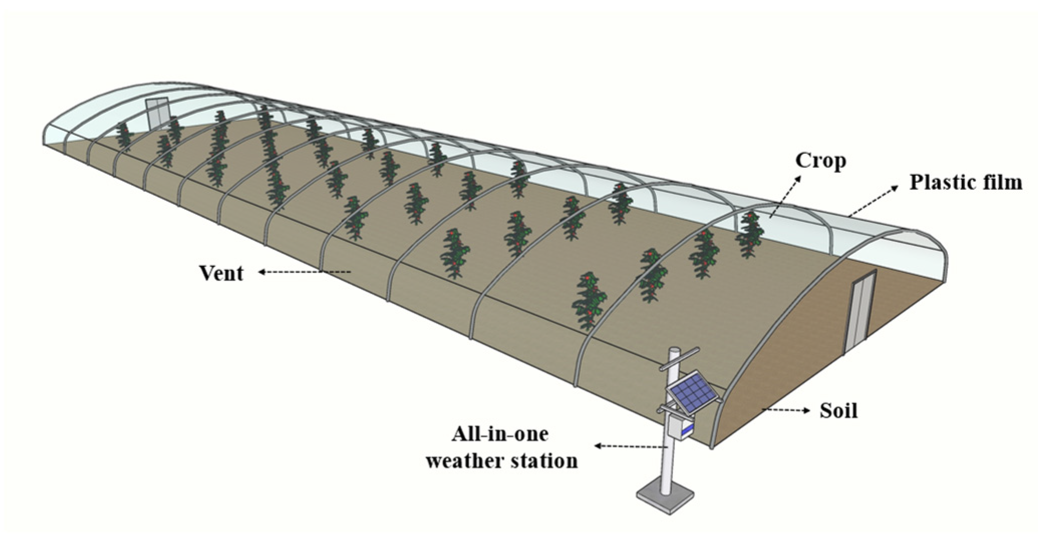
2.1. Description of the Experimental Greenhouse

Single-span plastic greenhouses were characterized by a simple arch design, often constructed from lightweight materials such as galvanized steel or aluminum. They were covered with transparent or translucent plastic film, allowing for optimal light penetration. Additionally, they facilitated effective ventilation through installed side and roof vents, which helped maintain optimal growing conditions. The experimental greenhouse was a single-span plastic greenhouse located in the National Agricultural Science and Technology Innovation Park in the Chengguan District, Lhasa, Tibet Autonomous Region (29°65′ N, 91°13′ E, with an average altitude of 3650 m). Its main structure was supported by a steel pipe arch, and the surrounding and top covering materials were PO film with a thickness of 0.10 mm, without insulation measures. The structure of the experimental greenhouse is shown in Figure 1. The greenhouse was symmetrically distributed in a circular arch shape, facing south, with an east-west orientation, and occupying an area of 691.2 m², with a length of 48.0 m, a span of 14.4 m, and a height of 2.5 m. There were two side vents in the greenhouse, located on the south and north sides, with an opening width of 1.0 m. The crop type planted was tomato, with an average plant height of 0.8 m, a plant spacing of 0.2 m, a plant density of 5 plants per square meter, rows oriented toward the south, and a leaf area index of 2.6.

2.2. Experimental Contents

First, the researchers understood the ventilation management mode of the experimental greenhouse (ventilation from 9:00 to 20:00 and closed at other times) and the environmental characteristics of the surrounding area and measured the basic structural dimensions of the greenhouse and crop morphological parameters. Next, based on the structural features of the greenhouse and the layout of the vents, they determined the distribution of environmental data monitoring points, as well as the types and quantities of sensors. Finally, they calibrated and installed the sensors. Considering the remote location of the experimental site and the need for long-term data monitoring, a comprehensive environmental monitoring cloud platform based on RS-485 bus technology was set up.

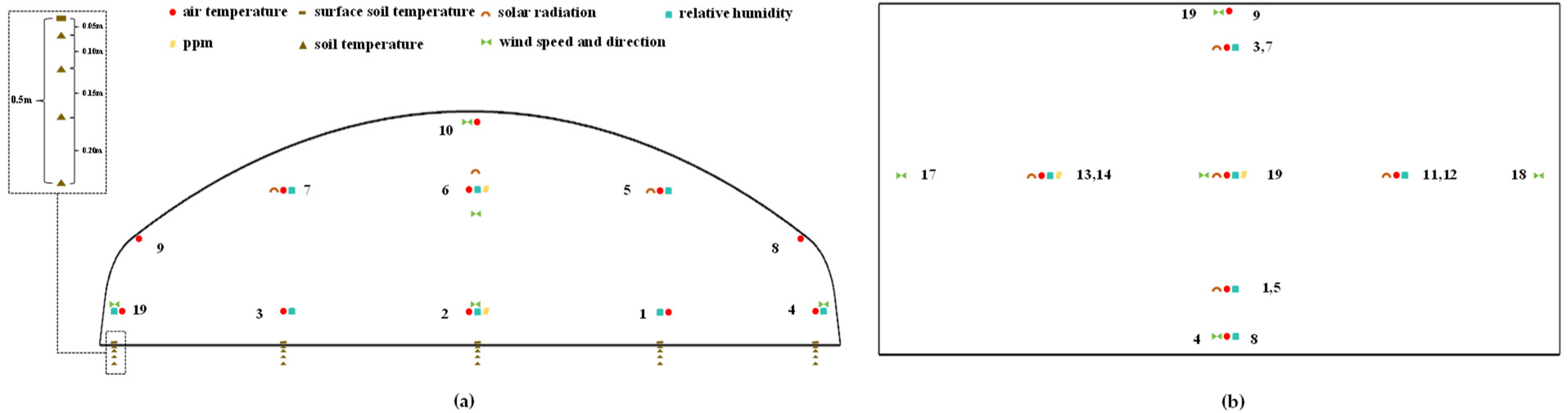
2.3. Environmental Data Collection

The measured environmental parameters included wind speed, indoor and outdoor air temperature, solar radiation, relative humidity, plastic film temperature, and soil surface temperature. The temperature sensor used was the KZW/P-010 (PT100), the solar total radiation sensor was the RS-RA-NO1-AL, the wind speed sensor was the RS-FSJT-I20, and the relative humidity sensor was the RS-WS-I20-2-4. The YC1002 temperature module was utilized to collect temperature data, while the YC100 current module was used to gather other parameters. Due to the remote location of the Tibet region, all data were wirelessly transmitted via the 485-4G model to the cloud platform for remote collection, with a data collection interval of 10 min. The specific parameters of the sensors are shown in

Table 1. Sensor specifications.

Instrument	Measurement Data	Measurement Range	Precision
PT100	Temperature	−40~80 °C	±0.2 °C (25 °C)
Humidity sensor	Humidity	0~99%RH	±3%RH (5%RH~95%RH, 25 °C)
Thermal bulb wind speed sensor	Velocity	0~10 m/s	±(0.03 m/s + 2%reading)
Light sensor	Total indoor radiation	0~2000 W/m2	±10 W/m2

.

To account for the spatial and temporal variations of environmental factors inside the greenhouse, monitoring points were arranged both horizontally and vertically, with corresponding types of sensors installed. The layout of the monitoring points is shown in Figure 2.

2.4. CFD Model

2.4.1. Basic Control Equations

No matter how complex the flow situation was, it was controlled by the following three basic physical principles: the law of conservation of mass, Newton’s second law, and the law of conservation of energy. These three basic physical principles corresponded to three control equations, namely, the continuity equation, the momentum equation, and the energy equation. The process of discretizing the control equations using the finite volume method could be described in the following general form [15]:

$${\displaystyle \frac{\mathit{\partial }\left(\mathsf{\rho }\mathsf{\varphi }\right)}{\mathit{\partial }\mathrm{t}}}+\mathrm{d}\mathrm{i}\mathrm{v}\left(\mathsf{\rho }\mathrm{u}\mathsf{\varphi }\right)=\mathrm{d}\mathrm{i}\mathrm{v}\left(\mathsf{\Gamma }\mathrm{g}\mathrm{r}\mathrm{a}\mathrm{d}\mathsf{\varphi }\right)+{\mathrm{S}}_{\mathsf{\Phi }}$$

(1)

In the equation, ρ was the fluid density, $\mathrm{k}\mathrm{g}·{\mathrm{m}}^{-3}$; $\mathsf{\varphi }$ was the general variable that represented the solved variables, such as velocity components and temperature; $\mathrm{u}$ was the fluid velocity, $\mathrm{m}·{\mathrm{s}}^{-1}$; Γ was the generalized diffusion coefficient; and ${\mathrm{S}}_{\mathsf{\Phi }}$ was the generalized source term.

2.4.2. Boussinesq Approximation

During the convective heat transfer process between plants and the surrounding structure and air, a buoyancy term due to density differences arose. To handle this term, the following assumptions, known as the Boussinesq approximation [16,17], were made: ① the physical properties other than density were assumed to be constant; ② the viscous dissipation in the fluid was neglected; and ③ only the density in terms related to volumetric forces in the momentum equation was considered, while the density in other terms was assumed to be constant.

2.4.3. Turbulence Model

In the natural ventilation process, the airflow exhibited obvious turbulent characteristics [18]. The gas inside the greenhouse could be considered a low-speed, continuous, and incompressible fluid with turbulent properties [19]. In recent years, the standard k-ε model had been widely used in related research [20]. However, considering the high-altitude and low-air pressure characteristics of the experimental area, for turbulent flow in low-pressure environments, it was better to choose the RNG k-ε model, which offered high simulation accuracy and good convergence [21]. This model reflected the influence of small-scale motion within the large-scale motion and included the modified viscosity term. The turbulence model is presented in Equations (2) and (3).

$${\displaystyle \frac{\mathit{\partial }}{\mathit{\partial }\mathrm{t}}}\left(\mathsf{\rho }\mathrm{k}\right)+{\displaystyle \frac{\mathit{\partial }}{\mathit{\partial }{\mathrm{x}}_{\mathrm{i}}}}\left(\mathsf{\rho }\mathrm{k}{\mathrm{u}}_{\mathrm{i}}\right)={\displaystyle \frac{\mathit{\partial }}{\mathit{\partial }{\mathrm{x}}_{\mathrm{j}}}}\left({\mathsf{\alpha }}_{\mathrm{k}}{\mathsf{\mu }}_{\mathrm{e}\mathrm{f}\mathrm{f}}{\displaystyle \frac{\mathit{\partial }\mathrm{k}}{\mathit{\partial }{\mathrm{x}}_{\mathrm{j}}}}\right)+{\mathrm{G}}_{\mathrm{k}}+{\mathrm{G}}_{\mathrm{b}}-\mathsf{\rho }\mathsf{\epsilon }-{\mathrm{Y}}_{\mathrm{m}}+{\mathrm{S}}_{\mathrm{k}}$$

(2)

$${\displaystyle \frac{\mathit{\partial }}{\mathit{\partial }\mathrm{t}}}\left(\mathsf{\rho }\mathsf{\epsilon }\right)+{\displaystyle \frac{\mathit{\partial }}{\mathit{\partial }{\mathrm{x}}_{\mathrm{i}}}}\left(\mathsf{\rho }\mathsf{\epsilon }{\mathrm{u}}_{\mathrm{i}}\right)={\displaystyle \frac{\mathit{\partial }}{\mathit{\partial }{\mathrm{x}}_{\mathrm{j}}}}\left({\mathsf{\alpha }}_{\mathsf{\epsilon }}{\mathsf{\mu }}_{\mathrm{e}\mathrm{f}\mathrm{f}}{\displaystyle \frac{\mathit{\partial }\mathsf{\epsilon }}{\mathit{\partial }{\mathrm{x}}_{\mathrm{j}}}}\right)+{\mathrm{C}}_1{\displaystyle \frac{\mathsf{\epsilon }}{\mathrm{k}}}\left({\mathrm{G}}_{\mathrm{k}}+{\mathrm{C}}_2{\mathrm{G}}_{\mathrm{b}}\right)+{\mathrm{C}}_3\mathsf{\rho }{\displaystyle \frac{{\mathsf{\epsilon }}^2}{\mathrm{k}}}-{\mathrm{R}}_{\mathsf{\epsilon }}+{\mathrm{S}}_{\mathsf{\epsilon }}$$

(3)

In the equation, G_k was the generation term of turbulent kinetic energy k caused by the average velocity gradient; G_b was the turbulent kinetic energy generated by buoyancy; Y_m was the fluctuation generated by excessive diffusion in a compressible flow, with a value of 0; C_l, C₂, and C₃ were model constants; ${\mathsf{\alpha }}_{\mathrm{k}}$ and ${\mathsf{\alpha }}_{\mathsf{\epsilon }}$ were the turbulent Prandtl numbers for the two equations; and ${\mathrm{S}}_{\mathrm{k}}$ and ${\mathrm{S}}_{\mathsf{\epsilon }}$ were custom terms.

2.4.4. Solar Radiation Model

Sunlight served as a vital energy source in the greenhouse, significantly influencing the spatial and temporal distribution of temperature, as well as the characteristics of the flow field within. Additionally, radiation heat exchange occurred between the greenhouse and the surrounding environment, warranting its consideration in the calculations. In high-altitude areas, air density is notably lower, leading to variations in radiation behavior and heat transfer mechanisms. The discrete ordinates radiation model (DO) effectively addresses these factors by providing a more accurate representation of radiative transfer in the atmosphere, particularly concerning scattering and absorption characteristics. This ensures reliable predictions of temperature distribution and heat exchange processes, which are crucial for modeling high-altitude scenarios. Consequently, the DO model was employed to account for the influence of solar radiation, with the specific equation detailed as follows [12,22]:

$$\nabla ·\left(\mathrm{I}\left(\overrightarrow{\mathrm{r}},\overrightarrow{\mathrm{s}}\right)\overrightarrow{\mathrm{s}}\right)+\left(\mathrm{a}+{\mathsf{\sigma }}_{\mathrm{s}}\right)·\mathrm{I}\left(\overrightarrow{\mathrm{r}},\overrightarrow{\mathrm{s}}\right)=\mathrm{a}{·\mathrm{n}}^2·{\displaystyle \frac{\mathsf{\sigma }{\mathrm{T}}^4}{\mathsf{\pi }}}+{\displaystyle \frac{{\mathsf{\sigma }}_{\mathrm{s}}}{4\mathsf{\pi }}}{\int }_0^{4\mathsf{\pi }}\mathsf{\Phi }\left(\overrightarrow{\mathrm{s}},{\overrightarrow{\mathrm{s}}}^{\prime }\right)·\mathrm{I}\left(\overrightarrow{\mathrm{s}},{\overrightarrow{\mathrm{s}}}^{\prime }\right)·\mathrm{d}{\mathsf{\Omega }}^{\prime }$$

(4)

In the equation, $\overrightarrow{\mathrm{r}}$ was the position vector; $\overrightarrow{\mathrm{s}}$ was the direction vector; ${\overrightarrow{\mathrm{s}}}^{\prime }$ was the refraction coefficient; $\mathrm{a}$ was the absorption coefficient; $\mathrm{n}$ was the refractive coefficient; $\mathsf{\sigma }$ was the Stefan-Boltzmann constant, also known as the blackbody radiation constant, with a value of $5.672\times {10}^{-8}\mathrm{W}·({\mathrm{m}}^{-2}·{\mathrm{K}}^{-4})$; ${\mathsf{\sigma }}_{\mathrm{s}}$ was the scattering coefficient; $\mathrm{I}$ was the total solar radiation intensity on the horizontal surface, $\mathrm{W}·{\mathrm{m}}^{-2}$; $\mathsf{\Phi }$ was the phase function; and ${\mathsf{\Omega }}^{\prime }$ was the solid angle of radiation, which equaled ${180}^2/{\mathsf{\pi }}^2$.

2.4.5. Species Transport Model

Air served as a medium for heat transfer and energy exchange among the atmosphere, greenhouse, and crops, primarily consisting of a mixture of water vapor and dry air. During the natural ventilation process, the indoor moist air is continuously convected and diffused with the external environment through airflow. In the numerical calculations, it was assumed that the humidity levels of the air both inside and outside the greenhouse reached a steady state. The species transport model was as follows:

$${\displaystyle \frac{\mathit{\partial }\left(\mathsf{\rho }{\mathrm{C}}_{\mathrm{s}}\right)}{\mathit{\partial }\mathrm{t}}}+\mathrm{d}\mathrm{i}\mathrm{v}\left(\mathsf{\rho }\mathrm{u}{\mathrm{C}}_{\mathrm{s}}\right)=\mathrm{d}\mathrm{i}\mathrm{v}\left({\mathrm{D}}_{\mathrm{s}}\mathrm{g}\mathrm{r}\mathrm{a}\mathrm{d}\left(\mathsf{\rho }{\mathrm{C}}_{\mathrm{s}}\right)\right)+{\mathrm{S}}_{\mathrm{s}}$$

(5)

In the equation, ${\mathrm{C}}_{\mathrm{s}}$ was the volumetric concentration of species S, $\mathrm{k}\mathrm{g}·{\mathrm{m}}^{-3}$; ${\mathrm{D}}_{\mathrm{s}}$ was the diffusion coefficient of the species, ${\mathrm{m}}^2·{\mathrm{s}}^{-1}$; and ${\mathrm{S}}_{\mathrm{s}}$ was the mass of the species produced per unit volume by chemical reactions within the system per unit time, also known as the production rate, $\mathrm{k}\mathrm{g}·{\mathrm{s}}^{-1}·{\mathrm{m}}^{-3}$.

2.4.6. Crop Model

In order to describe the resistance effect of tomato crops on the airflow inside the greenhouse under natural ventilation conditions, tomatoes were considered an isotropic porous medium [23]. Following the Darcy-Forchheimer law, their impact was represented by adding a source term to the momentum equation, which was primarily composed of viscous resistance and flow inertia resistance. The model equation is presented as Equation (6) [17,24].

$${\mathrm{S}}_{\mathsf{\Phi }1}=\left(-{\displaystyle \frac{1}{\mathrm{K}}}\mathsf{\mu }\mathrm{u}\right)+\left(-{\displaystyle \frac{1}{2}}\mathsf{\rho }{\mathrm{Y}}_{\mathrm{u}}\left|\mathrm{u}\right|\mathrm{u}\right)$$

(6)

In the equation, ${\mathrm{S}}_{\mathsf{\Phi }1}$ was the source term of the momentum equation; $\mathrm{K}$ was the permeability of the porous medium model, ${\mathrm{m}}^2$, with a value of 0.395 [25]; the viscous resistance coefficient was denoted as ${\mathrm{X}}_{\mathrm{u}}$, where ${\mathrm{X}}_{\mathrm{u}}$ and $\mathrm{K}$ were reciprocals of each other, ${\mathrm{m}}^{-2}$, with a value of 2.532; and ${\mathrm{Y}}_{\mathrm{u}}$ was the inertia resistance coefficient, ${\mathrm{m}}^{-1}$.

The expression describing the relationship between pressure drop and viscous resistance when gas flowed through the tomato crop area inside the greenhouse was as follows [25]:

$${\displaystyle \frac{\mathit{\partial }\mathrm{P}}{\mathit{\partial }\mathrm{x}}}=-{\displaystyle \frac{1}{\mathsf{\mu }}}\mathrm{K}\mathrm{u}+{\displaystyle \frac{1}{\sqrt{\mathrm{K}}}}\mathsf{\rho }{\mathrm{Y}}_{\mathrm{u}}{\mathrm{u}}^2$$

(7)

In the equation, $\mathrm{P}$ was the pressure, Pa, and $\mathrm{x}$ was the thickness of the porous medium through which the indoor gas flowed, m.

Assuming that pressure was the main component of the total resistance in the canopy layer of the crop area [26], the equation for pressure drop was as follows [25]:

$${\displaystyle \frac{\mathit{\partial }\mathrm{P}}{\mathit{\partial }\mathrm{x}}}={\mathsf{\rho }\mathrm{C}}_{\mathrm{D}}{\mathrm{L}}_{\mathrm{A}\mathrm{D}}{\mathrm{u}}^2$$

(8)

In the equation, ${\mathrm{C}}_{\mathrm{D}}$ was the drag coefficient, with a value of 0.2 [25], and ${\mathrm{L}}_{\mathrm{A}\mathrm{D}}$ was the leaf area density, ${\mathrm{m}}^2/{\mathrm{m}}^3$.

By jointly deriving Equations (7) and (8), the expression for the inertia resistance coefficient ${\mathrm{Y}}_{\mathrm{u}}$ was obtained.

$${\mathrm{Y}}_{\mathrm{u}}={\mathrm{C}}_{\mathrm{D}}{\mathrm{L}}_{\mathrm{A}\mathrm{D}}{\mathrm{K}}^{0.5}$$

(9)

It was observed that when the pressure drop data of the gas passing through the crop area was obtained, the aerodynamic characteristics of the porous medium region could be calculated.

In the process of greenhouse ventilation control, in addition to mass exchange, energy exchange also occurs. To reflect the heat exchange between the crops and the surrounding air (including sensible heat and latent heat), it was added as a source term to the energy equation, as shown in Equation (10) [16,27].

$${\mathrm{S}}_{\mathsf{\Phi }2}=2{\rho }_a{\mathsf{\beta }}_{\mathrm{L}\mathrm{A}\mathrm{I}}{\mathrm{C}}_{\mathrm{p}}{\displaystyle \frac{{\mathrm{T}}_{\mathrm{c}}-{\mathrm{T}}_{\mathrm{i}}}{{\mathrm{r}}_{\mathrm{a}}}}+\mathsf{\lambda }{\rho }_a{\mathsf{\beta }}_{\mathrm{L}\mathrm{A}\mathrm{I}}{\displaystyle \frac{{\mathrm{H}}_{\mathrm{c}}-{\mathrm{H}}_{\mathrm{a}}}{{\mathrm{r}}_{\mathrm{a}}+{\mathrm{r}}_{\mathrm{s}}}}$$

(10)

In the equation, ${\mathrm{S}}_{\mathsf{\Phi }2}$ was the source term of the energy equation; ${\mathsf{\rho }}_{\mathrm{a}}$ was the air density, $\mathrm{k}\mathrm{g}·{\mathrm{m}}^{-3}$; ${\mathrm{C}}_{\mathrm{p}}$ was the specific heat capacity, $\mathrm{J}·({\mathrm{k}\mathrm{g}}^{-1}·{\mathrm{K}}^{-1})$; ${\mathrm{T}}_{\mathrm{c}}$ and ${\mathrm{T}}_{\mathrm{i}}$ were the temperature of the crop and indoor air, respectively, $\mathrm{K}$; $\mathsf{\lambda }$ was the latent heat of water evaporation, $\mathrm{J}·{\mathrm{k}\mathrm{g}}^{-1}$; ${\mathrm{r}}_{\mathrm{a}}$ and ${\mathrm{r}}_{\mathrm{s}}$ were the aerodynamic resistance of the crop boundary layer and the average resistance of crop stomata, respectively, $\mathrm{s}·{\mathrm{m}}^{-1}$; and ${\mathrm{H}}_{\mathrm{c}}$ and ${\mathrm{H}}_{\mathrm{a}}$ were the relative humidity of the crop and indoor air, respectively.

${\mathrm{r}}_{\mathrm{a}}$ and ${\mathrm{r}}_{\mathrm{s}}$ were calculated according to Equations (11) and (12), respectively [12,17].

$${\mathrm{r}}_{\mathrm{a}}=\left\{\begin{array}{ll}840{\left({\displaystyle \frac{\mathrm{d}}{\left|{\mathrm{T}}_{\mathrm{c}}-{\mathrm{T}}_{\mathrm{i}}\right|}}\right)}^{0.25}& \mathrm{u}<0.1\mathrm{m}/\mathrm{s}\\ 220\left({\displaystyle \frac{{\mathrm{d}}^{0.2}}{{\mathrm{u}}^{0.8}}}\right)& \mathrm{u}>0.1\mathrm{m}/\mathrm{s}\end{array}\right.$$

(11)

$${\mathrm{r}}_{\mathrm{s}}=200\left(1+{\displaystyle \frac{1}{{\mathrm{e}}^{0.05\left({\mathrm{R}\mathrm{a}}_{\mathrm{g}\mathrm{i}}-50\right)}}}\right)·\left(1+0.11{\mathrm{e}}^{\left(0.34{\displaystyle \frac{{\mathrm{D}}_{\mathrm{i}}}{100}}-10\right)}\right)$$

(12)

In the equation, $\mathrm{d}$ was the characteristic leaf length per unit length, m; ${\mathrm{R}\mathrm{a}}_{\mathrm{g}\mathrm{i}}$ was the internal solar radiation, $\mathrm{W}·{\mathrm{m}}^{-2}$; and ${\mathrm{D}}_{\mathrm{i}}$ was the saturation vapor pressure difference, ${\mathrm{P}}_{\mathrm{a}}$.

2.5. Numerical Calculation

2.5.1. Boundary Conditions and Calculation Parameters

The ventilation and heat exchange process was simulated, with the windward and leeward sides of the outflow domain set as the velocity inlet and pressure outlet, respectively. The sides and top were designated as symmetry planes, while the greenhouse cover layer was treated as a semi-transparent wall surface, with its inlet and outlet vents configured as internal surfaces. The inside and outside ground were established as wall boundary conditions. The outflow domain, greenhouse gas region, and crop area were defined as separate fluid domains. Field data collected on the cloud platform was extracted and processed, compiling environmental parameters such as wind speed, temperature, and solar radiation intensity into the solver. Taking the natural ventilation numerical model in this study as an example, the basic parameters of related materials are presented in

Table 2. Basic parameters of greenhouse materials.

Material	Density (kg·m−3)	Specific Heat Capacity (J·kg−1·K−1)	Thermal Conductivity (W·m−1·K−1)
Air	0.77	1005.57	0.026
Soil	1700	1010	0.80
Crop	560	2100	0.19
Plastic Film	950	1600	0.29

[12].

The efficiency of the computational process for fluid flow and heat transfer problems, as well as the accuracy of the numerical results, mainly depended on the grid and algorithms used [28]. In this study, the SIMPLEC algorithm was chosen for the coupled calculation of the pressure and velocity fields. In the spatial discretization of the CFD model, the gradients were calculated using the least squares method; the energy and momentum terms utilized a second-order upwind scheme, and the RNG k-ε turbulence model employed first-order discretization for turbulent coordinates, turbulent kinetic energy, and turbulent dissipation rate. The walls were set as no-slip wall conditions, and near-wall treatment was implemented using the standard wall function method [20]. The curvature correction function was activated to enhance the gradient accuracy of the selected gradient method and expedite the convergence process of the calculations. The residual values for the continuity, turbulence, radiation, and energy equations were set to 10⁻³, 10⁻³, 10⁻³, and 10⁻⁸, respectively.

2.5.2. Geometric Modeling and Grid Generation

Three-dimensional modeling software was used to create a 1:1 parameterized solid model of the greenhouse, in which each row of tomato crops was simplified into a hexahedral region measuring 2.85 m (length) × 0.7 m (width) × 0.8 m (height). To avoid backflow effects, the approach proposed by Lee et al. [29] was typically employed, positioning the leeward side of the outflow field at least 15 ${\mathrm{H}}_{\mathrm{g}}$ away from the greenhouse, while the other sides were required to maintain a distance of at least 5 ${\mathrm{H}}_{\mathrm{g}}$, where ${\mathrm{H}}_{\mathrm{g}}$ represented the ridge height of the arched greenhouse. After the modeling was completed, the model was imported into the fluent meshing module for grid generation. In the meshing process, to reduce computational costs and enhance accuracy, surface meshes with local sizes were initially set, followed by geometric discretization of the computational domain using the polyhedral mesh partitioning method. Considering the complex flow conditions in the ventilation openings and crop areas, as well as the significant velocity gradients near the walls, appropriate refinement was applied to these areas, resulting in a total of 2,979,356 volume meshes. The maximum mesh skewness was 0.75, with an average element quality of 0.85, indicating good mesh partitioning quality that met the requirements for subsequent calculations. The three-dimensional model and grid layout are shown in Figure 3.

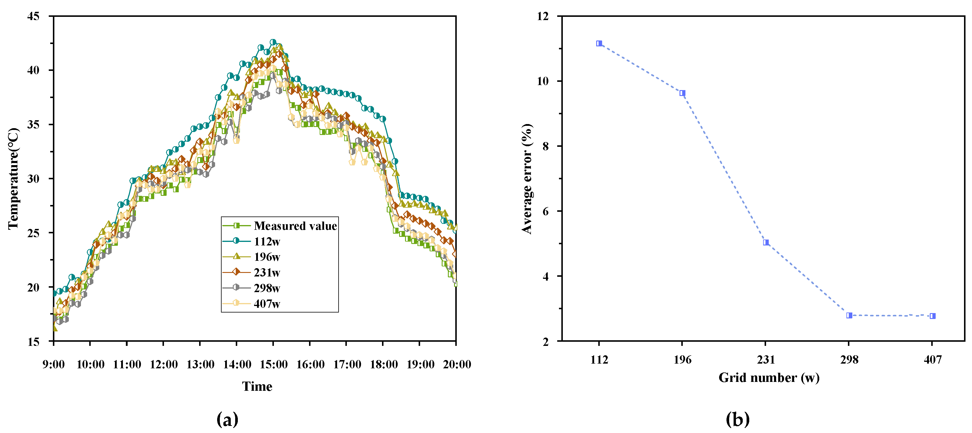
2.5.3. Grid Independence Validation

For the transient calculation, it was necessary to verify that the results were independent of the grid quantity. To confirm grid independence, five CFD models with varying levels of grid refinement were created, and numerical calculations were performed under the same conditions. The volume mesh quantities for these models were 1.12 million, 1.96 million, 2.31 million, 2.98 million, and 4.07 million. The calculation results for the average indoor temperature and the error analysis are presented in Figure 4.

The maximum errors between the measured and simulated values of the indoor average temperature for the CFD models with 2.98 million and 4.07 million meshes were 4.51% and 4.86%, with average errors of 2.82% and 2.68%, all below 5%. Therefore, it was concluded that grid independence had been achieved. However, considering both solution accuracy and computational efficiency, the CFD model with 2.98 million meshes was selected for further research.

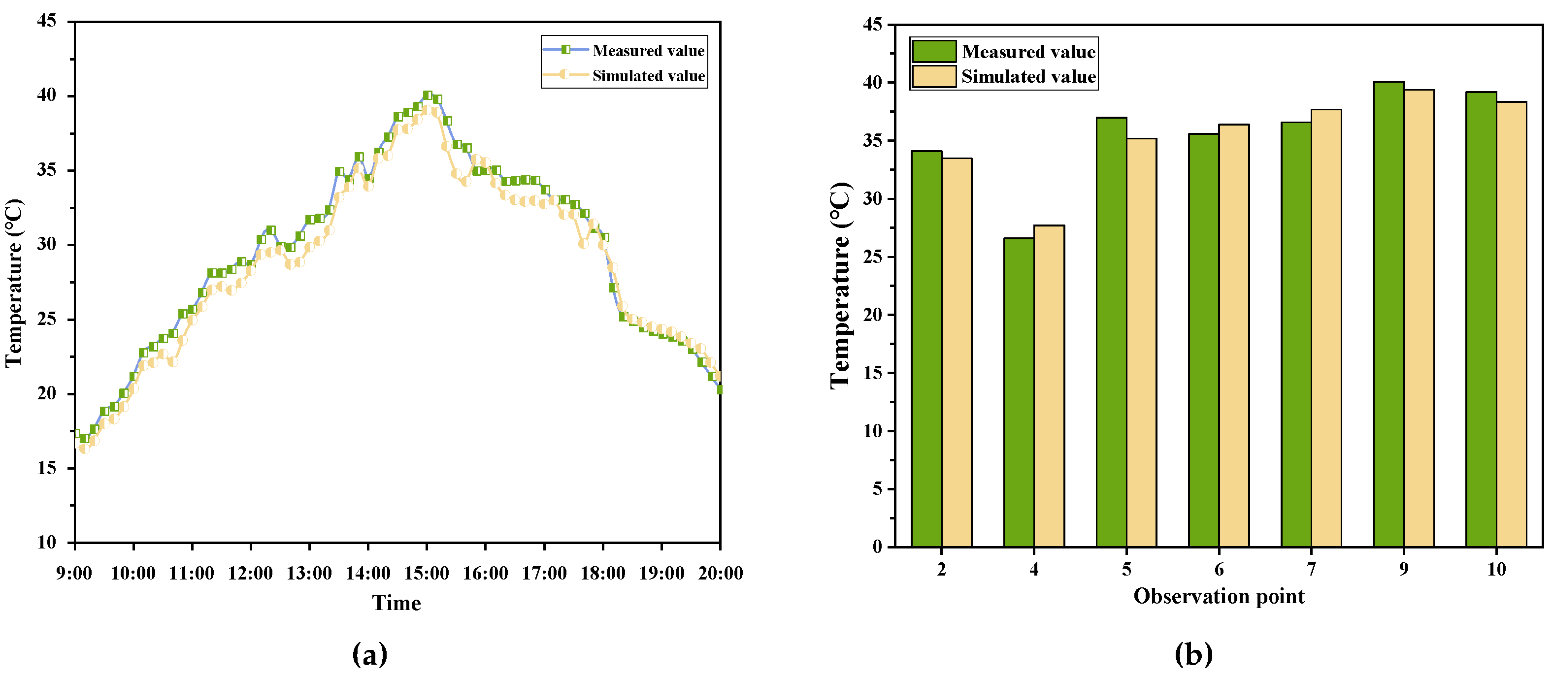
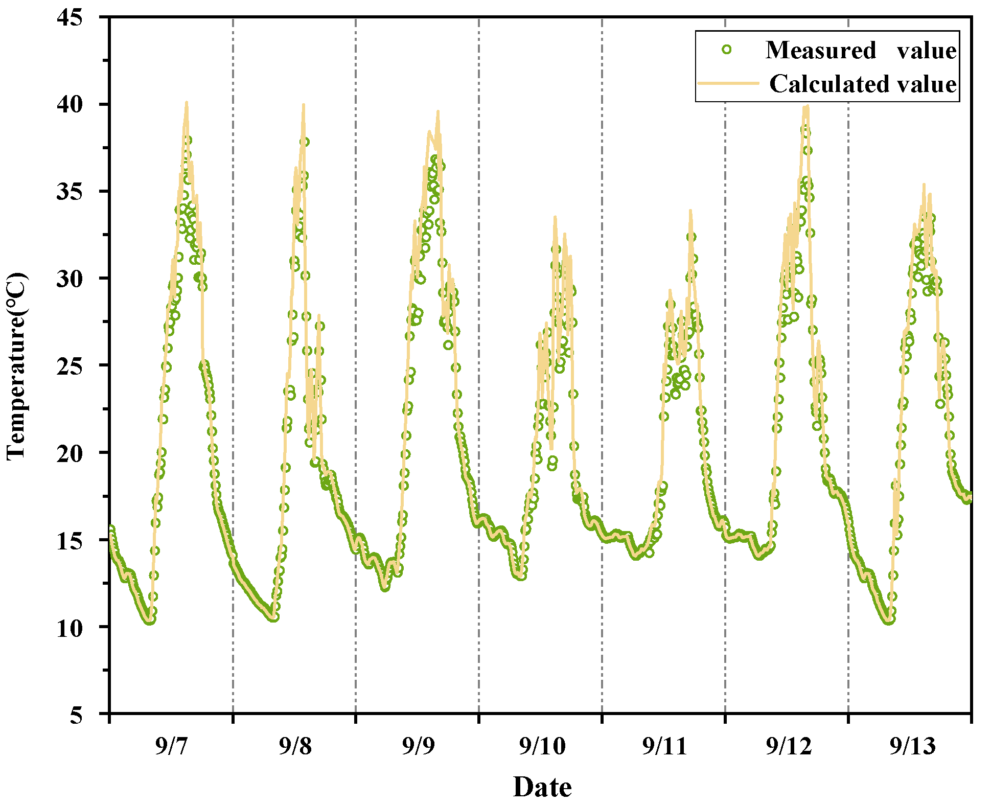
2.5.4. Model Validation

Indoor and outdoor meteorological parameters during the ventilation period of a typical sunny day (from 9:00 to 20:00 on 7 September 2022) were used to simulate the natural ventilation process of the experimental greenhouse. To thoroughly validate the reliability of the established model and the numerical calculation methods employed, we analyzed the measured and simulated indoor temperatures from both temporal and spatial perspectives, with the results presented in Figure 5. Figure 5a illustrates the temporal variation of the average indoor temperature, while Figure 5b depicts the temperature distribution at various measurement points within the greenhouse.

Typically, the mean absolute error (MAE), mean relative error (MRE), root mean square error (RMSE), and coefficient of determination (R²) were used to measure the fit between the two. In the error analysis, Figure 5a indicated that the MAE was 0.99 °C, the MRE was 3.43%, the RMSE was 1.12 °C, and the R² was 0.9832. Similarly, Figure 5b presented an MAE of 1.39 °C, an MRE of 4%, an RMSE of 1.25 °C, and an R² of 0.9707. These results demonstrated a strong agreement between the measured and simulated values, suggesting that the established model and its associated numerical calculation methods were reliable.

3. Results and Discussion

3.1. Analysis of Factors Affecting Ventilation Rate

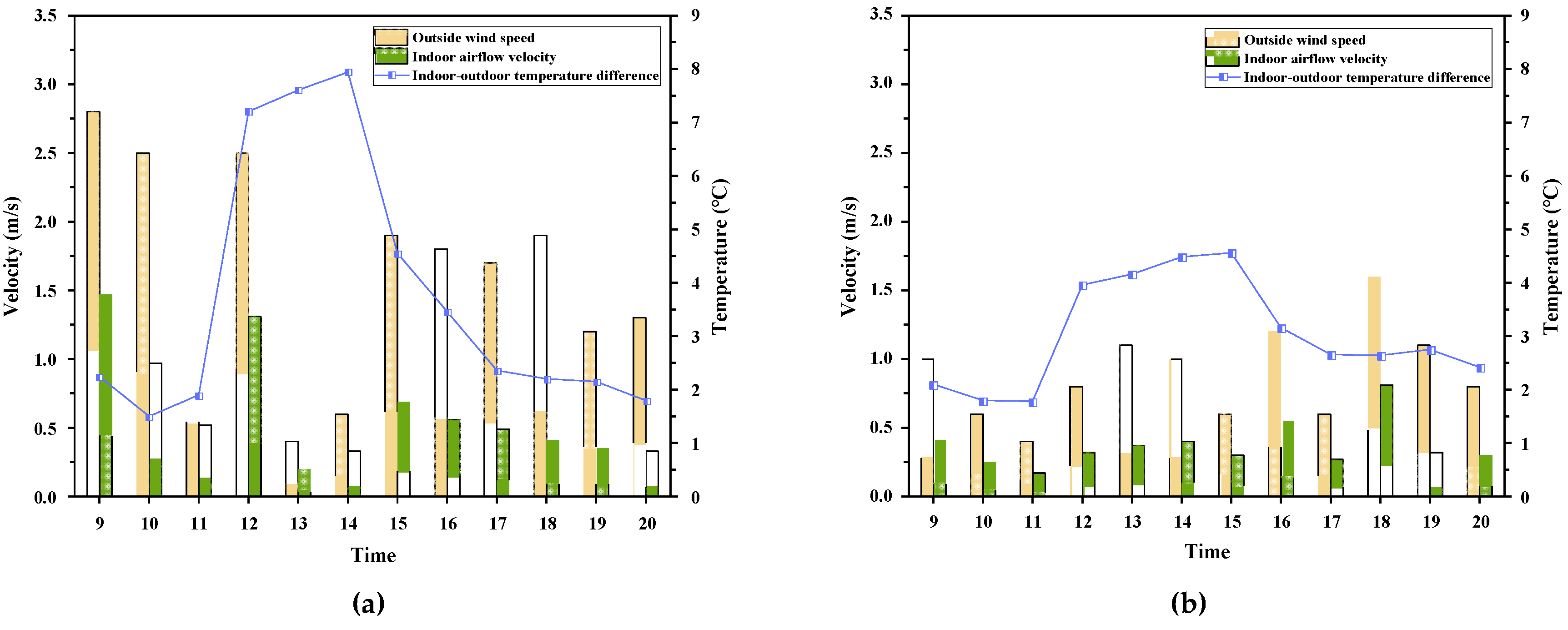
3.1.1. Daily Variation Patterns of Indoor Air Velocity

Due to the fact that air velocity can intuitively reflect changes in ventilation rates, the variations of indoor air velocity with outdoor wind speeds and indoor-outdoor temperature differences were analyzed under the following two conditions: sunny and cloudy days. Based on the relationship between different weather conditions and solar radiation intensity [11], 7 September was identified as a sunny day, and 11 September was identified as a cloudy day. The daily variation patterns of indoor air velocity are shown in Figure 6.

Regardless of whether it is sunny or cloudy, there is a strong correlation between indoor air velocity and outside wind speed. The indoor-outdoor temperature difference shows a trend of initially decreasing slowly, then increasing, and finally decreasing. Under the same outside wind speed conditions, when the indoor-outdoor temperature difference is large, the indoor air velocity also increases, generally following a pattern of increasing with a larger temperature difference. However, the relationship between the two is not very pronounced.

3.1.2. Correlation Analysis and Significance Testing

Apart from outside wind speed and indoor-outdoor temperature difference, natural ventilation is also influenced by factors such as the density difference between indoor and outdoor air, total indoor radiation, and the evapotranspiration of plants. Therefore, it is necessary to conduct a correlation analysis and significance test (with a significance level of p ≤ 0.01) on factors affecting ventilation. The results are presented in the form of a heatmap, as shown in Figure 7.

The correlation coefficient ${\mathsf{\rho }}_{\mathrm{r}}$ of the outside wind speed is 0.83, showing a significant relationship with ventilation. The correlation coefficient of the indoor-outdoor temperature difference is 0.31, ranking second in influence among the factors, following outside wind speed. Considering the thermal pressure effect caused by the indoor-outdoor temperature difference under certain conditions, which affects natural ventilation, it is believed that the variation in greenhouse ventilation is influenced by the indoor-outdoor temperature difference. Therefore, the combined effects of the outside wind speed and indoor-outdoor temperature difference should be considered in the construction of the ventilation model.

3.2. Ventilation Rate Model

Currently, research on greenhouse ventilation is mainly focused on low-altitude regions, with relatively limited studies conducted in high-altitude areas. This paper aims to establish a ventilation model for single-span plastic greenhouses suitable for high-altitude areas, optimizing ventilation management to enhance the quality of the crop growth environment.

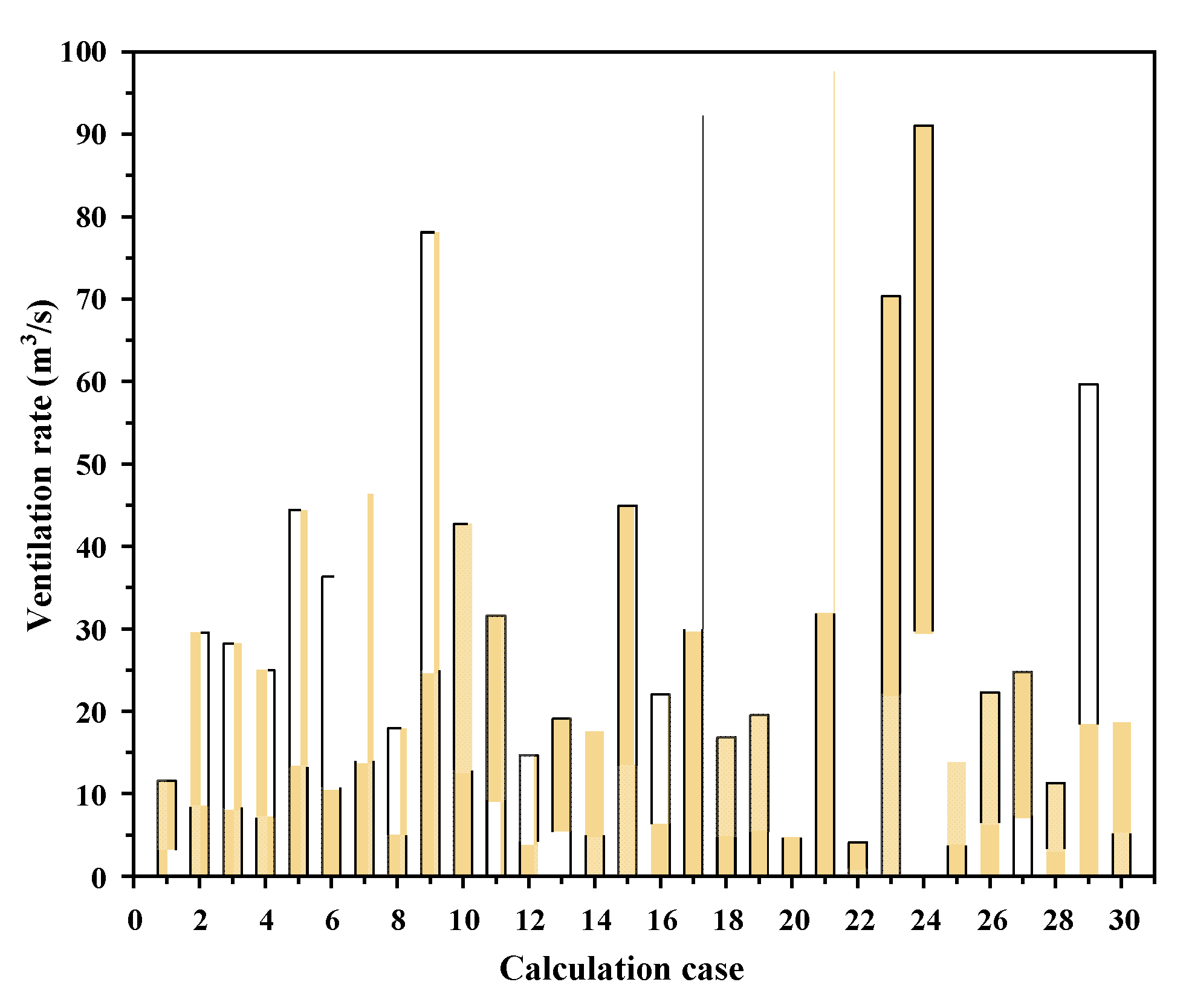
3.2.1. Ventilation Rate Sample Values

To establish the ventilation rate model, 30 sets of operating conditions in September were selected for analysis. Monitoring points were set at the outlet of the model to measure the ventilation rate, providing data support for the subsequent model establishment. The ventilation rate sample values are shown in Figure 8.

3.2.2. Ventilation Rate Model Establishment

Assuming the airflow velocity at the inlet is $\mathrm{v}$, the relationship between wind pressure and inlet velocity can be obtained using Bernoulli’s equation [30].

$$∆{\mathrm{P}}_{\mathrm{w}}={\displaystyle \frac{1}{2}}{\mathsf{\rho }}_{\mathrm{a}}{\mathrm{C}}_{\mathrm{w}}{\mathrm{v}}^2$$

(13)

In the equation, $∆{\mathrm{P}}_{\mathrm{w}}$ is the indoor-outdoor pressure difference at the ventilation opening caused by outside wind speed, ${\mathrm{P}}_{\mathrm{a}}$; ${\mathrm{C}}_{\mathrm{w}}$ is the wind pressure shape coefficient; and $\mathrm{v}$ is the inlet velocity, $\mathrm{m}·{\mathrm{s}}^{-1}$.

Ventilation under thermal pressure is mainly related to temperature variations at different height positions. Thermal pressure can be represented by Equation (14) [30].

$$∆{\mathrm{P}}_{\mathrm{s}}={\mathsf{\rho }}_{\mathrm{a}}\mathrm{g}\mathrm{H}{\displaystyle \frac{∆\mathrm{T}}{\mathrm{T}}}$$

(14)

In the equation, $∆{\mathrm{P}}_{\mathrm{s}}$ is the indoor-outdoor pressure difference at the ventilation opening caused by the indoor-outdoor temperature difference, P_a; g is the acceleration due to gravity, with a value of 9.8 $\mathrm{m}·{\mathrm{s}}^{-2}$; $\mathrm{H}$ is the reference height, m; T is the outdoor air temperature, K; and ∆T is the indoor-outdoor temperature difference, K.

T. Boulard et al. [31,32] found in their experiments on arched greenhouse ventilation that the most accurate ventilation model is achieved by combining the thermal pressure ventilation rate with the wind pressure ventilation rate.

$$\mathrm{G}={\mathrm{G}}_{\mathrm{s}}+{\mathrm{G}}_{\mathrm{w}}$$

(15)

$$\mathrm{G}={\displaystyle \frac{{\mathrm{A}}_{\mathrm{s}}}{2}}{\mathrm{C}}_{\mathrm{q}}{\left[{\displaystyle \frac{\mathrm{g}}{2}}\left({\displaystyle \frac{∆\mathrm{T}}{\mathrm{T}}}\right)\mathrm{H}\right]}^{0.5}+{\displaystyle \frac{{\mathrm{A}}_{\mathrm{s}}}{2}}{\mathrm{C}}_{\mathrm{q}}{\left({\mathrm{C}}_{\mathrm{w}}\right)}^{0.5}\mathrm{v}$$

(16)

In the equation, G is the wind pressure-thermal pressure coupled ventilation rate, ${\mathrm{m}}^3·{\mathrm{s}}^{-1}$; ${\mathrm{G}}_{\mathrm{s}}$ is the thermal pressure ventilation rate, ${\mathrm{m}}^3·{\mathrm{s}}^{-1}$; ${\mathrm{G}}_{\mathrm{w}}$ is the wind pressure ventilation rate, ${\mathrm{m}}^3·{\mathrm{s}}^{-1}$; ${\mathrm{A}}_{\mathrm{s}}$ is the ventilation opening area, ${\mathrm{m}}^2$; and ${\mathrm{C}}_{\mathrm{q}}$ is the airflow coefficient of the ventilation opening. Let ${\mathrm{C}}_{\mathrm{q}}{\left({\mathrm{C}}_{\mathrm{w}}\right)}^{0.5}$ represent the wind effect adjustment factor, which describes the dynamic adjustment capability of the greenhouse ventilation system under specific wind field conditions.

Equation (16) represents the ventilation model for single-span plastic greenhouses at high altitudes when naturally ventilated. This model takes into account the unique environmental conditions of the local area. By utilizing the Lsqcurvefit toolbox to perform a multivariate nonlinear function fitting on the ventilation sample data, the values of ${\mathrm{C}}_{\mathrm{q}}$ and ${\mathrm{C}}_{\mathrm{q}}{\left({\mathrm{C}}_{\mathrm{w}}\right)}^{0.5}$ are obtained. An error analysis is also conducted on the sample ventilation values and the fitted values, with the related results shown in

Table 3. Error analysis of sample value and fitting value of greenhouse ventilation.

Cq	Cq (Cw)0.5	MAE (m3·s−1)	ARE (%)	RMSE (m3·s−1)	R2
0.0955	0.6258	0.5257	3.27	0.6501	0.9996

.

3.3. Ventilation Rate Model Validation

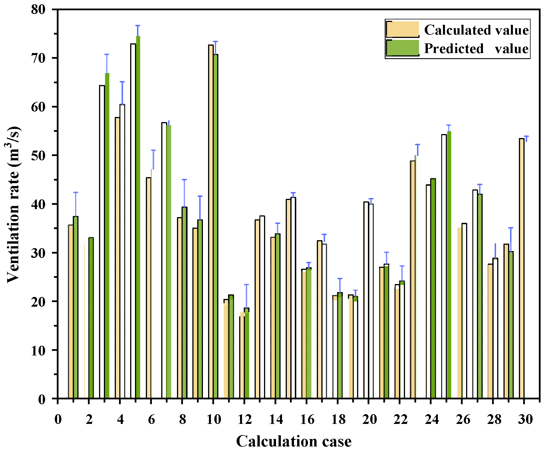
3.3.1. Accuracy Validation

The purpose of greenhouse ventilation is to optimize internal environmental conditions, meet the growth requirements of crops, and improve crop yield and quality. One of the key functions is to remove excess heat through ventilation, preventing the indoor temperature from rising too high and creating a suitable growth environment. Therefore, to verify whether the ventilation rate calculated based on Equation (16) can remove the excess heat indoors, an energy balance analysis of the indoor air is required.

Considering the uneven distribution of internal environmental space, a three-dimensional numerical model is needed for simulation. However, to simplify the complexity of calculations, a one-dimensional heat transfer model [33] is chosen. Based on this, the following basic assumptions are made:

(1) Assuming complete mixing of indoor air, neglecting density changes;

(2) Assuming a uniform distribution of solar radiation intensity inside the greenhouse;

(3) Since tomato fruits have a water content exceeding 90%, it is assumed that the thermal properties of crops are the same as those of water.

The indoor air mainly exchanges heat through convection with the covering materials, soil, and crops and exchanges heat with the outdoor air through natural ventilation. The energy changes in indoor air include ① convective heat exchange between indoor air and the covering layer (${\mathsf{\Phi }}_{\mathrm{a}\mathrm{p}}$); ② convective heat exchange between indoor air and the soil surface (${\mathsf{\Phi }}_{\mathrm{a}\mathrm{s}}$); ③ convective heat exchange between indoor air and crops (${\mathsf{\Phi }}_{\mathrm{a}\mathrm{c}}$); ④ heat flow caused by ventilation between indoor and outdoor air (${\mathsf{\Phi }}_{\mathrm{a}\mathrm{w}}$); and ⑤ heat flow caused by cold air infiltration (${\mathsf{\Phi }}_{\mathrm{a}\mathrm{l}}$).

The energy balance equation is as follows:

$${\mathsf{\rho }}_{\mathrm{a}}{\mathrm{C}}_{\mathrm{a}\mathrm{p}}{\mathrm{V}}_{\mathrm{a}}{\displaystyle \frac{\mathrm{d}{\mathrm{T}}_{\mathrm{a}}}{\mathrm{d}\mathrm{t}}}={\mathsf{\Phi }}_{\mathrm{a}\mathrm{p}}+{\mathsf{\Phi }}_{\mathrm{a}\mathrm{s}}-{\mathsf{\Phi }}_{\mathrm{a}\mathrm{c}}-{\mathsf{\Phi }}_{\mathrm{a}\mathrm{w}}-{\mathsf{\Phi }}_{\mathrm{a}\mathrm{l}}$$

(17)

In the equation, ${\mathrm{C}}_{\mathrm{a}\mathrm{p}}$ is the specific heat of air at constant pressure, $\mathrm{J}·\left({\mathrm{k}\mathrm{g}}^{-1}·{\mathrm{K}}^{-1}\right)$; ${\mathrm{V}}_{\mathrm{a}}$ is the volume of indoor air, ${\mathrm{m}}^3$; ${\mathrm{T}}_{\mathrm{a}}$ is the indoor air temperature, K; $\mathrm{t}$ is time, $\mathrm{s}$; and ${\displaystyle \frac{\mathrm{d}{\mathrm{T}}_{\mathrm{a}}}{\mathrm{d}\mathrm{t}}}$ is the rate of change in indoor air temperature per unit time.

The calculation equations for each energy exchange term are as follows:

$${\mathsf{\Phi }}_{\mathrm{a}\mathrm{p}}={\mathrm{h}}_{\mathrm{a}\mathrm{p}}·{\mathrm{A}}_{\mathrm{p}}·\left({\mathrm{T}}_{\mathrm{p}}-{\mathrm{T}}_{\mathrm{a}}\right)$$

(18)

$${\mathsf{\Phi }}_{\mathrm{a}\mathrm{s}}={\mathrm{h}}_{\mathrm{a}\mathrm{s}}·{\mathrm{A}}_{\mathrm{s}}·\left({\mathrm{T}}_{\mathrm{s}}-{\mathrm{T}}_{\mathrm{a}}\right)$$

(19)

$${\mathsf{\Phi }}_{\mathrm{a}\mathrm{c}}={\mathrm{h}}_{\mathrm{a}\mathrm{c}}·{\mathrm{A}}_{\mathrm{c}}·\left({\mathrm{T}}_{\mathrm{a}}-{\mathrm{T}}_{\mathrm{c}}\right)$$

(20)

$${\mathsf{\Phi }}_{\mathrm{a}\mathrm{w}}={\mathsf{\rho }}_{\mathrm{a}}{·\mathrm{C}}_{\mathrm{a}\mathrm{p}}·\mathrm{G}·\left({\mathrm{T}}_{\mathrm{a}}-{\mathrm{T}}_{\mathrm{o}}\right)$$

(21)

In the equation, ${\mathrm{h}}_{\mathrm{a}\mathrm{p}}$ is the convective heat transfer coefficient between indoor air and the inner surface of the covering layer, $\mathrm{W}·\left({\mathrm{m}}^{-1}·{\mathrm{K}}^{-1}\right)$; ${\mathrm{h}}_{\mathrm{a}\mathrm{s}}$ is the convective heat transfer coefficient between indoor air and the soil surface, $\mathrm{W}·\left({\mathrm{m}}^{-1}·{\mathrm{K}}^{-1}\right)$; ${\mathrm{h}}_{\mathrm{a}\mathrm{c}}$ is the convective heat transfer coefficient between indoor air and the crop surface, $\mathrm{W}·\left({\mathrm{m}}^{-1}·{\mathrm{K}}^{-1}\right)$; ${\mathrm{A}}_{\mathrm{p}}$ is the surface area of the greenhouse covering layer, ${\mathrm{m}}^2$; ${\mathrm{A}}_{\mathrm{s}}$ is the ground area inside the greenhouse, ${\mathrm{m}}^2$; ${\mathrm{A}}_{\mathrm{c}}$ is the surface area of the crops inside the greenhouse, ${\mathrm{m}}^2$; $\mathrm{G}$ is the natural ventilation rate of the greenhouse, ${\mathrm{m}}^3·{\mathrm{s}}^{-1}$; ${\mathrm{T}}_{\mathrm{p}}$ is the temperature of the inner surface of the greenhouse covering layer, K; ${\mathrm{T}}_{\mathrm{s}}$ is the temperature of the ground inside the greenhouse, K; and ${\mathrm{T}}_{\mathrm{c}}$ is the temperature of the crop surface inside the greenhouse, K. Since the heat flow from cold air infiltration is significantly smaller than that from ventilation, its neglect facilitates the simplification of the indoor air energy balance equation while maintaining calculation accuracy. Additionally, a previous study [33] has demonstrated that the impact of cold air infiltration on the energy balance of indoor air is generally negligible compared to that of ventilation. Therefore, ${\mathsf{\Phi }}_{\mathrm{a}\mathrm{l}}$ can be omitted in this context.

Simulating the indoor air temperature variations based on the energy balance model, an error analysis is conducted on the measured and simulated values to validate the accuracy of the model. Representative data from 7 September to 13 September 2022, are selected for analysis, with a day defined as 0:00 to 24:00. The dates of 10, 11, and 13 September were cloudy days, while the remaining days were sunny. The analysis results are shown in Figure 9.

Tibet is located on a plateau with thin air, strong daytime sunlight, rapid heat absorption by indoor air during the day leading to temperature rise, and fast heat loss at night causing rapid temperature drop, resulting in significant day-night temperature differences. The simulated indoor air temperature during the day is lower than the actual values, which is attributed to the omission of energy losses from heat conduction and convection between indoor and outdoor air through the covering layer in the construction of the indoor air energy balance model, considering the greenhouse lacks insulation and has a single-layer film covering. MAE, MRE, RMSE, and ${\mathrm{R}}^2$ between measured and simulated values are 0.8139 °C, 3.19%, 1.3738 °C, and 0.9792, respectively, demonstrating the model’s accuracy in simulating the heat flow induced by ventilation. This energy balance model can be used for predicting and evaluating changes in greenhouse indoor air temperature.

3.3.2. Applicability Validation

To validate the applicability of the ventilation rate model under different environmental conditions, the predicted values are compared with the calculated values, and the model’s predictive performance is shown in Figure 10.

The MAE, MRE, RMSE, and ${\mathrm{R}}^2$ between predicted and calculated values are 0.7706 ${\mathrm{m}}^3·{\mathrm{s}}^{-1}$, 3.18%, 1.1449 ${\mathrm{m}}^3·{\mathrm{s}}^{-1}$, and 0.9995, respectively. These values indicate that the model has high predictive accuracy, providing an effective calculation tool for natural ventilation systems in high-altitude areas. The ventilation rate model can be expressed as Equation (22).

$$\mathrm{G}=0.048{\mathrm{A}}_{\mathrm{s}}{·\left[{\displaystyle \frac{\mathrm{g}}{2}}\left({\displaystyle \frac{∆\mathrm{T}}{\mathrm{T}}}\right)\mathrm{H}\right]}^{0.5}+0.31{\mathrm{A}}_{\mathrm{s}}·\mathrm{v}$$

(22)

In the equation, $\mathrm{G}$ is the wind pressure-thermal pressure coupled ventilation rate, ${\mathrm{m}}^3·{\mathrm{s}}^{-1}$; ${\mathrm{A}}_{\mathrm{s}}$ is the ground area inside the greenhouse, ${\mathrm{m}}^2$; $\mathrm{g}$ is the acceleration due to gravity, with a value of 9.8 $\mathrm{m}·{\mathrm{s}}^{-2}$; $\mathrm{T}$ is the outdoor air temperature, $\mathrm{K}$; $∆\mathrm{T}$ is the indoor-outdoor temperature difference, $\mathrm{K}$; $\mathrm{H}$ is the reference height, $\mathrm{m}$; and $\mathrm{v}$ is the inlet velocity, $\mathrm{m}·{\mathrm{s}}^{-1}$.

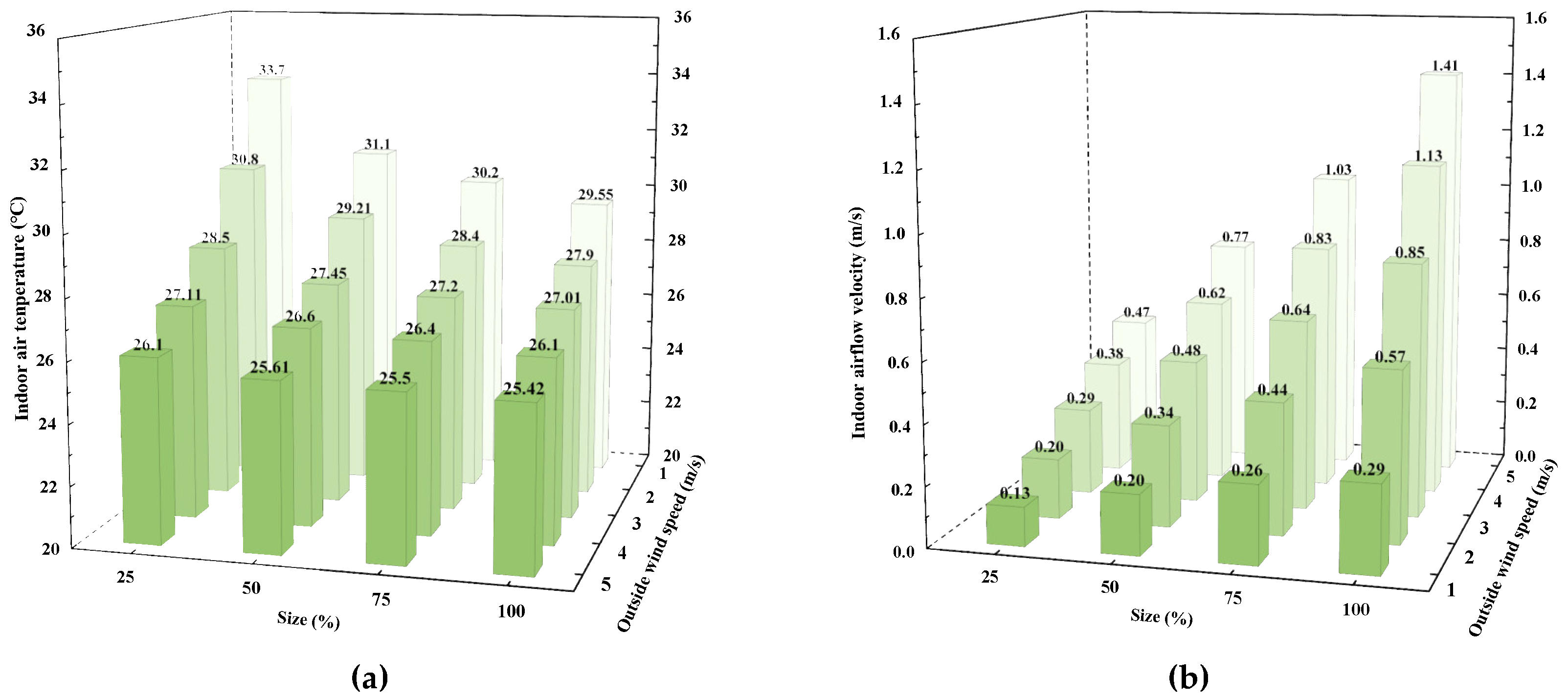
3.4. The Impact of Ventilation Opening Sizes

Using the environmental parameters from 13 September 2022 as boundary conditions for a numerical solution, we simulated the variations in indoor average flow velocity and average temperature under different outside wind speeds and ventilation opening sizes. The calculation results after 10 min of ventilation are shown in Figure 11. After statistical analysis of the outdoor environmental parameters, it is found that outside wind speeds mainly range from 0 to 5 m/s. To reduce the additional impact of thermal pressure on ventilation effectiveness based on the research related to the threshold wind speed values, outside wind speeds of 1, 2, 3, 4, and 5 m/s were selected for this study.

The calculation results of indoor average air temperature under different outside wind speeds and ventilation opening sizes are shown in Figure 11a. Regardless of how the outside wind speed varies, the trend of indoor average air temperature with varying ventilation opening sizes remains consistent, showing an overall inverse relationship. The indoor temperature at a 25% ventilation opening is higher than at other opening sizes, indicating that the smaller the ventilation opening, the harder it is to lower the indoor temperature. Additionally, when the ventilation opening size remains constant, the indoor average air temperature decreases with increasing outside wind speed. When the outside wind speed is below 3 m/s, it has a significant impact on the indoor average temperature, with temperature ranges of 5.2 °C, 3.65 °C, 3 °C, and 2.54 °C for the four opening conditions. When the outside wind speed exceeds 3 m/s, the airflow inside the greenhouse develops fully, leading to a relatively stable indoor average air temperature that is less affected by significant changes in outside wind speed. In terms of the indoor average air temperature, the optimal ventilation opening size for cooling is between 75% and 100%.

From Figure 11b, it can be observed that the indoor average airflow velocity varies with the vent opening size under different outside wind speeds. When the outside wind speed remains constant and the ventilation opening size increases, the indoor average airflow velocity also increases. For outside wind speeds of 1, 2, 3, 4, and 5 m/s, the range of indoor airflow average velocity is 0.16 m/s, 0.37 m/s, 0.56 m/s, 0.75 m/s, and 0.94 m/s respectively, indicating its dependence on outside wind speed. When the outside wind speed is low, the effect of ventilation opening size on indoor average airflow velocity is not significant. This is because the ventilation opening height is close to the crop canopy height, and the crops have a certain blocking effect on airflow. Additionally, the greenhouse has a large span, resulting in a minor impact of ventilation opening size on indoor airflow. For tomatoes, the suitable indoor airflow velocity for growth is 0.5–1 m/s [34]. Therefore, to meet the environmental requirements for tomato growth, it is recommended to keep the greenhouse ventilation fully open when the outside wind speed is below 1 m/s; when the outside wind speed is between 1 and 3 m/s, the greenhouse ventilation opening should be set at 75–100%, and when the outside wind speed exceeds 3 m/s, the recommended greenhouse ventilation opening is 25–75%.

To precisely control the climate conditions inside the greenhouse, this paper proposed a ventilation model with different ventilation opening sizes based on Equation (22), aiming to enhance the natural ventilation system in high-altitude areas. This model, based on fluid dynamics and thermodynamic principles, comprehensively considers key parameters such as the greenhouse geometry, outside wind speed, indoor-outdoor temperature difference, and ventilation opening size to quantitatively describe their relationship with the ventilation rate. By applying the model, greenhouse managers can be provided with a theoretical basis to optimize ventilation strategies. Furthermore, in subsequent studies, this model can be integrated into automated control systems to dynamically adjust ventilation opening sizes, automatically respond to environmental changes, and meet real-time crop growth requirements. Therefore, the ventilation rate model for different ventilation opening sizes of single-span plastic greenhouses in high-altitude areas is shown in Equation (24).

$${\mathsf{\lambda }}_{\mathrm{h}}=0.92{\mathrm{f}}_{\mathrm{o}\mathrm{p}\mathrm{e}\mathrm{n}}+0.09$$

(23)

$${\mathrm{G}}_{\mathrm{h}}={\mathsf{\lambda }}_{\mathrm{h}}\left(0.048{\mathrm{A}}_{\mathrm{s}}{·\left[{\displaystyle \frac{\mathrm{g}}{2}}\left({\displaystyle \frac{∆\mathrm{T}}{\mathrm{T}}}\right)\mathrm{H}\right]}^{0.5}+0.31{\mathrm{A}}_{\mathrm{s}}·\mathrm{v}\right)$$

(24)

In the equation, ${\mathsf{\lambda }}_{\mathrm{h}}$ is the opening-related coefficient; ${\mathrm{f}}_{\mathrm{o}\mathrm{p}\mathrm{e}\mathrm{n}}$ is the ventilation opening size; and ${\mathrm{G}}_{\mathrm{h}}$ is the ventilation airflow under different ventilation opening sizes, ${\mathrm{m}}^3·{\mathrm{s}}^{-1}$.

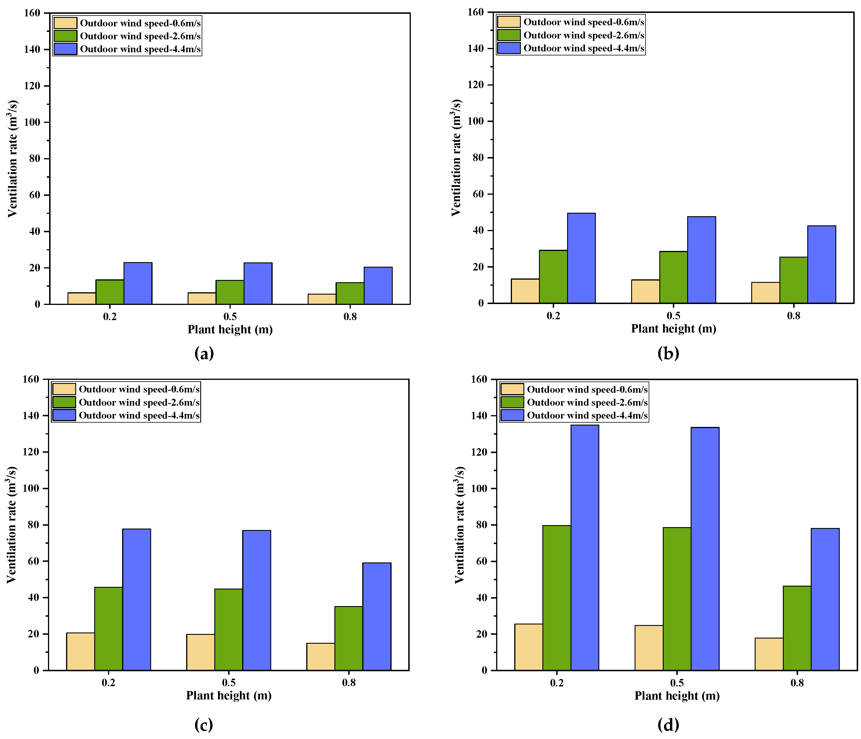
3.5. The Impact of Plant Heights

Based on Section 3.4, the natural ventilation process of the experimental greenhouse under different plant heights was simulated using the indoor and outdoor environmental parameters from 13 September 2022. Considering the characteristics of different growth stages of the crops, this study selected plant heights of 0.2 m, 0.5 m, and 0.8 m. The calculation results are presented in Figure 12.

From Figure 12, it is evident that the greenhouse ventilation rate generally decreases as plant height increases, indicating a negative correlation between the two. However, this correlation is not significant when the plant height is relatively low. For instance, a 4% reduction in ventilation rate was observed as the plant height grew from 0.2 m to 0.5 m under the conditions of a 100% ventilation opening size and an outdoor wind speed of 4.4 m/s.

Furthermore, the relationship between the ventilation opening size and ventilation rate also varies with changes in plant height. When the plant height increases from 0.2 m to 0.5 m, the reduction in the ventilation rate remains within 4%, regardless of variations in outdoor wind speed and ventilation opening size, suggesting that the impact of plant height on the ventilation rate is not significant when it is less than 0.5 m. However, as plant height increases from 0.5 m to 0.8 m, the reduction in ventilation rate exceeds 10%. Notably, when the ventilation opening size is greater than 75%, the reduction in ventilation rate under low, medium, and high wind speed conditions exceeds 20%. This indicates that at this height, the plants significantly obstruct airflow, resulting in a substantial decrease in ventilation rate.

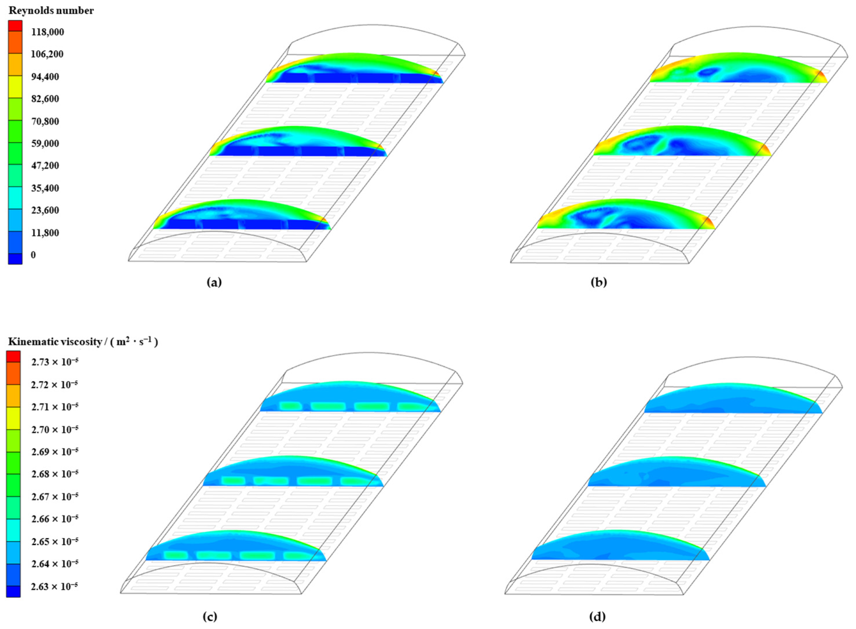
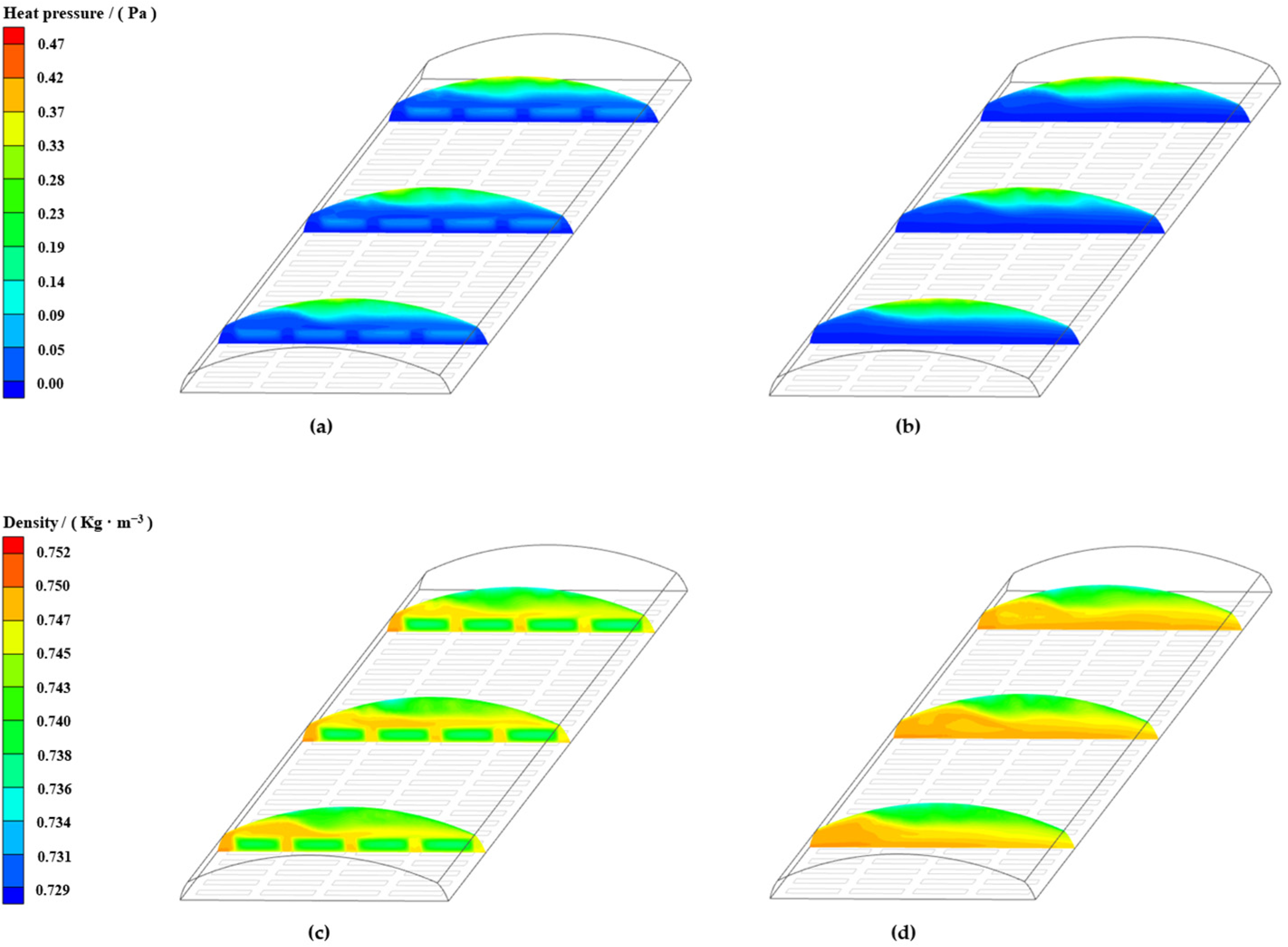
3.6. Analysis of Natural Ventilation Characteristics

The proportion of the influence of thermal pressure and wind pressure in natural ventilation depends on the outside wind speed [35]. Considering the environmental characteristics of high-altitude areas, it is necessary to determine the threshold wind speed values for natural ventilation types in the context of this study. Additionally, a single-layer plastic film cannot withstand the low temperatures of winter, thus failing to provide suitable growth conditions to support crop production during the winter season. Therefore, the greenhouse is only operational in spring, summer, and autumn. Under varying environmental conditions, the magnitude of the ventilation rate generated by thermal pressure and wind pressure can differ significantly. Therefore, it is crucial to compare the ventilation rates resulting from both thermal and wind pressure to identify the threshold wind speeds at which each effect becomes dominant. Specifically, when the wind speed exceeds a certain threshold, the ventilation rate within the greenhouse is primarily influenced by the external wind speed. In contrast, when the wind speed falls below this threshold, thermal pressure predominantly governs the ventilation rate. The proportion of the wind pressure ventilation rate to the total ventilation rate was analyzed using Equation (22), and the results are presented in Figure 13, which encompasses data from three quarters.

As shown in Figure 13, when the outside wind speed exceeds 1.0 $\mathrm{m}·{\mathrm{s}}^{-1}$, the wind pressure ventilation volume accounts for 70% of the total ventilation volume, indicating a predominance of wind pressure. In contrast, when the outside wind speed drops below 0.3 $\mathrm{m}·{\mathrm{s}}^{-1}$, the wind pressure ventilation volume comprises less than 30% of the total, with thermal pressure ventilation becoming the primary mode. When the outside wind speed falls between these two values, the ventilation is characterized by a coupling of wind pressure and thermal pressure. Thus, the threshold wind speed values that categorize the natural ventilation types in single-span plastic greenhouses in high-altitude areas can be determined.

Based on the obtained boundary wind speed values, we further investigated the natural ventilation characteristics. The boundary conditions of the CFD model are shown in

Table 4. Main calculation boundary conditions.

Outside Wind Speed (m·s−1)	Outside Air Temperature (°C)	Outside Soil Temperature (°C)	Inside Air Temperature (°C)	Inside Soil Temperature (°C)	Plastic Film Temperature (°C)
1.6	19.4	23.6	21.5	19.3	30.0
0.2	26.4	24.9	32.5	28.0	39.1
0.7	27.5	26.3	29.4	26.9	32.9

.

3.6.1. Wind Pressure Ventilation

Wind pressure ventilation is a method that utilizes outside wind forces to promote airflow through pressure differences. In the analysis of wind pressure ventilation, the focus is primarily on the indoor convective flow caused by the inflow of outside air, while neglecting the heat exchange between the greenhouse structure and the air, as well as the evapotranspiration of crops. In general, the distribution pattern of Re and kinematic viscosity can be used to reflect the characteristics of wind pressure ventilation, as shown in Figure 14.

Re is the ratio of fluid inertial force to viscous force, serving as a similarity criterion to characterize the impact of viscosity on fluid flow. By comparing the distribution patterns of Re for two types of cross-sections, it can be observed that in non-crop areas, Re is relatively high, typically above 10,000, indicating strong turbulent characteristics. In crop areas, except at the boundaries of crops, Re is below 2000, indicating laminar flow. Kinematic viscosity is the ratio of fluid dynamic viscosity to fluid density at the same temperature, representing the measure of viscous force during flow. The kinematic viscosity in crop areas is higher than in non-crop areas, indicating significant viscous effects in crop areas, hindering gas flow inside the greenhouse. In non-crop areas, the viscous force between adjacent fluid layers is smaller, leading to better gas flow conditions.

Both Re and kinematic viscosity show that the closer the distance to the inlet, the greater the difference between the crop area and the non-crop area. This is because the airflow is at its highest speed when it first enters the greenhouse. After being obstructed by the crops, it quickly changes its flow trajectory and becomes turbulent. As the flow develops further, this difference gradually diminishes.

3.6.2. Thermal Pressure Ventilation

Thermal pressure ventilation is a method that utilizes the pressure difference caused by the difference in air density between the indoors and outdoors to drive airflow and achieve ventilation. In the analysis of thermal pressure ventilation, the focus is primarily on the heat exchange between different parts inside the greenhouse and the surrounding air due to temperature differences. The characteristics of thermal pressure ventilation are typically related to thermal pressure and density. Figure 15 shows the distribution patterns of both.

In the non-crop area, the density shows a decreasing trend from bottom to top. This indicates that within the horizontal height range of the ventilation opening, the airflow is good, while above, due to the obstruction of flow and the influence of solar radiation, the temperature increases. The air, being heated and expanding, causes a decrease in density, making it lighter than the cooler air below, resulting in an upward buoyant force. This force drives the hot air to rise, which represents the mode of action for thermal pressure. However, in this plastic greenhouse without a top ventilation opening, the hot air cannot be expelled promptly and accumulates in the upper region, forming a high-pressure zone. The upper region of the greenhouse cannot efficiently exchange airflow with the outdoor environment, leading to reduced ventilation efficiency compared to wind-pressure ventilation.

3.6.3. Wind Pressure-Thermal Pressure Coupled Ventilation

Wind pressure-thermal pressure coupled ventilation is a method that utilizes indoor-outdoor temperature differences and wind forces to promote air. This method can demonstrate advantages in various environments and climate conditions, providing more stable and effective ventilation effects.

As shown in Figure 16, the temperature in the crop area is significant, mainly due to the porous nature of the crops themselves, which hinders the airflow and prevents effective heat dissipation. Additionally, as the experimental greenhouse only has side vents and lacks top vents, the airflow primarily moves rapidly at the horizontal height of the vents, creating a good flow state and heat exchange effect. However, this structure also leads to turbulent airflow movement in the upper part of the greenhouse, reducing ventilation and heat exchange efficiency. Consequently, the temperature inside the greenhouse increases from bottom to top, with temperatures getting higher the farther away from the vents. Moreover, the covering layer, which is heated directly by solar radiation, reaches temperatures exceeding 32 °C, further exacerbating this phenomenon.

4. Conclusions

This paper proposes a natural ventilation model for single-span plastic greenhouses in high-altitude areas using a combined approach of experimentation and numerical simulation. The following conclusions are drawn from the analysis:

Validation of the CFD numerical model with the measured data showed good consistency between measured and simulated values. Based on this, different boundary conditions were set for numerical simulations to extract ventilation rates. An empirical formula for natural ventilation rates was derived through nonlinear fitting, with an ${\mathrm{R}}^2$ of 0.9724. The accuracy of the ventilation rate formula was verified through an energy balance analysis of indoor air. The calculated ventilation rates from the formula precisely simulate the portion of heat removed during the ventilation process. Additionally, the energy balance equation established in this process can predict and evaluate air temperature changes inside single-span plastic greenhouses in high-altitude areas. By varying the size of greenhouse ventilation openings and conducting numerical simulations, a natural ventilation model under different opening conditions was established based on the formula for 100% opening. This provides an effective computational tool for controlling natural ventilation systems in high-altitude areas. Based on this analysis, we examined the relationship between plant height and ventilation rate, discovering that the greenhouse ventilation rate decreases as plant height increases, indicating a negative correlation between the two.

The threshold wind speed for distinguishing wind pressure ventilation, thermal pressure ventilation, and coupled ventilation was proposed for single-span plastic greenhouses in high-altitude areas. Specifically, wind pressure ventilation predominates when outdoor wind speeds exceed 1 $\mathrm{m}·{\mathrm{s}}^{-1}$; thermal pressure ventilation is dominant when outdoor wind speeds are below 0.3 $\mathrm{m}·{\mathrm{s}}^{-1}$; and when outdoor wind speeds range from 0.3 to 1 $\mathrm{m}·{\mathrm{s}}^{-1}$, the ventilation type is coupled ventilation.

References

1. Li, Q. Discussion on the Development of Facility Vegetables in Tibet under the Rural Revitalization Strategy. Tibet Agric. Sci. Technol. 2020, 2, 62–65. (In Chinese) [Google Scholar]
2. Cheng, F. Current Situation and Countermeasures of Facility Vegetable Development in Tibet Region. Anhui Agric. Bull. 2021, 27, 57–58. [Google Scholar] [CrossRef]
3. Lei, W.; Lu, H.; Qi, X.; Tai, C.; Fan, X.; Zhang, L. Field measurement of environmental parameters in solar greenhouses and analysis of the application of passive ventilation. Sol. Energy 2023, 263, 111851. [Google Scholar] [CrossRef]
4. Park, D.; Kang, B.; Cho, K.; Shin, C.; Cho, S.; Park, J.; Yang, W. A Study on Greenhouse Automatic Control System Based on Wireless Sensor Network. Wirel. Pers. Commun. 2011, 56, 117–130. [Google Scholar] [CrossRef]
5. Cao, K.; Xu, H.; Zhang, R.; Xu, D.; Yan, L.; Sun, Y.; Xia, L.; Zhao, J.; Zou, Z.; Bao, E. Renewable and sustainable strategies for improving the thermal environment of Chinese solar greenhouses. Energy Build. 2019, 202, 109414. [Google Scholar] [CrossRef]
6. Teitel, M.; Wenger, E. Air exchange and ventilation efficiencies of a monospan greenhouse with one inflow and one outflow through longitudinal side openings. Biosyst. Eng. 2014, 119, 98–107. [Google Scholar] [CrossRef]
7. Tusi, A.; Shimazu, T.; Ochiai, M.; Suzuki, K. Continuous Measurement of Greenhouse Ventilation Rate in Summer and Autumn via Heat and Water Vapor Balance Methods. Environ. Control Biol. 2021, 59, 41–48. [Google Scholar] [CrossRef]
8. Mashonjowa, E.; Ronsse, F.; Milford, J.R.; Lemeur, R.; Pieters, J.G. Measurement and simulation of the ventilation rates in a naturally ventilated Azrom-type greenhouse in Zimbabwe. Appl. Eng. Agric. 2010, 26, 475–488. [Google Scholar] [CrossRef]
9. Akrami, M.; Javadi, A.A.; Hassanein, M.J.; Farmani, R. Study of the effects of vent configuration on mono-span greenhouse ventilation using computational fluid dynamics. Sustainability 2020, 12, 986. [Google Scholar] [CrossRef]
10. Chu, C.R.; Lan, T.W.; Tasi, R.K.; Wu, T.R.; Yang, C.K. Wind-driven natural ventilation of greenhouses with vegetation. Biosyst. Eng. 2017, 164, 221–234. [Google Scholar] [CrossRef]
11. Yang, Z.; Zou, Z.; Chen, S.; Wang, J. Indoor Wind Speed Distribution in Northwestern Solar Greenhouses and its Relationship with Outdoor Wind Speed and Ventilation Area. J. Northwest AF Univ. 2006, 34, 36–40. [Google Scholar] [CrossRef]
12. Liang, B.; Zhao, S.; Li, Y.; Wang, P.; Liu, Z.; Zhang, J.; Ding, T. Study on the Natural Ventilation Characteristics of a Solar Greenhouse in a High-Altitude Area. Agronomy 2022, 12, 2387. [Google Scholar] [CrossRef]
13. Fuller, R.; Aye, L.; Zahnd, A.; Thakuri, S. Thermal evaluation of a greenhouse in a remote high-altitude area of Nepal. Int. Energy 2009, 10, 71–80. [Google Scholar]
14. Sun, X.; Wu, L.; Ma, Y.; Wang, R.; Song, B. Analysis of Temperature Variation in High-altitude Solar Greenhouses. Agric. Sci. 2023, 13, 257–263. [Google Scholar] [CrossRef]
15. Cemek, B.; Atis, A.; Küçüktopcu, E. Evaluation of temperature distribution in different greenhouse models using computational fluid dynamics (CFD). Anadolu J. Agric. Sci. 2017, 32, 54–63. [Google Scholar] [CrossRef]
16. Xu, F.; Cai, Y.; Chen, J.; Zhang, L. Temperature/flow field simulation and parameter optimal design for greenhouses with fan-pad evaporative cooling system. Trans. Chin. Soc. Agric. Eng. 2015, 31, 201–208. [Google Scholar] [CrossRef]
17. Wu, F.; Xu, F.; Zhang, L.; Ma, X. Numerical simulation on thermal environment of heated glass greenhouse based on porous medium. Trans. Chin. Soc. Agric. Eng. 2011, 42, 180–185. [Google Scholar]
18. Zhong, H.; Sun, Y.; Shang, J.; Qian, F.; Zhao, F.; Kikumoto, H.; Jimenez-Bescos, C.; Liu, X. Single-sided natural ventilation in buildings: A critical literature review. Build. Environ. 2022, 212, 108797. [Google Scholar] [CrossRef]
19. Velazquez, J.; Montero, J.; Montero, J.; Baeza, E.; Lopez, J. Mechanical and natural ventilation systems in a greenhouse designed using computational fluid dynamics. Int. J. Agric. Biol. Eng. 2014, 7, 1–16. [Google Scholar] [CrossRef]
20. Cemek, B.; Atis, A.; Küçüktopcu, E. Evaluation of various turbulence models performance for greenhouse simulation. In Proceedings of the Second International Symposium on Agricultural Engineering, Belgrade, Serbia, 9–10 October 2015; pp. 39–51. Available online: https://www.researchgate.net/publication/330114969 (accessed on 9 October 2015).
21. Küçüktopcu, E.; Cemek, B. Evaluating the influence of turbulence models used in computational fluid dynamics for the prediction of airflows inside poultry houses. Biosyst. Eng. 2019, 183, 1–12. [Google Scholar] [CrossRef]
22. Saberian, A.; Sajadiye, S. The effect of dynamic solar heat load on the greenhouse microclimate using CFD simulation. Renew. Energy 2019, 138, 722–737. [Google Scholar] [CrossRef]
23. Nurmalisa, M.; Tokairin, T.; Kumazaki, T.; Takayama, K.; Inoue, T. CO2 Distribution under CO2 Enrichment Using Computational Fluid Dynamics Considering Photosynthesis in a Tomato Greenhouse. Appl. Sci. 2022, 12, 7756. [Google Scholar] [CrossRef]
24. Kibwika, A.; Seo, H.; Seo, I. CFD Model Verification and Aerodynamic Analysis in Large-Scaled Venlo Greenhouse for Tomato Cultivation. AgriEngineering 2023, 5, 1395–1414. [Google Scholar] [CrossRef]
25. Kang, L.; Zhang, Y.; Kacira, M.; Hooff, T. CFD simulation of air distributions in a small multi-layer vertical farm: Impact of computational and physical parameters. Biosyst. Eng. 2024, 243, 148–174. [Google Scholar] [CrossRef]
26. Jiang, C.; Xu, K.; Rao, J.; Liu, J.; Li, Y.; Song, Y.; Li, M.; Zheng, Y.; Lu, W. Establishment and Solution of a Finite Element Gas Exchange Model in Greenhouse-Grown Tomatoes for Two-Dimensional Porous Media with Light Quantity and Light Direction. Agriculture 2024, 14, 1209. [Google Scholar] [CrossRef]
27. Miao, Z. Numerical Simulation and Optimization of Vent Configuration for Natural Ventilation of the Large Space Exhibition Greenhouse. Refrig. Air Cond. 2020, 34, 29–38. [Google Scholar] [CrossRef]
28. Li, H.; Li, Y.; Yue, X.; Liu, X.; Tian, S.; Li, T. Evaluation of airflow pattern and thermal behavior of the arched greenhouses with designed roof ventilation scenarios using CFD simulation. PLoS ONE 2020, 15, e0239851. [Google Scholar] [CrossRef]
29. Lee, S.; Lee, I.; Kim, R. Evaluation of wind-driven natural ventilation of single-span greenhouses built on reclaimed coastal land. Biosyst. Eng. 2018, 171, 120–142. [Google Scholar] [CrossRef]
30. Zhai, Z.; Mankibi, M.; Zoubir, A. Review of Natural Ventilation Models. Energy Procedia 2015, 78, 2700–2705. [Google Scholar] [CrossRef]
31. Teitel, M.; Liran, O.; Tanny, J.; Barak, M. Wind driven ventilation of a mono-span greenhouse with a rose crop and continuous screened side vents and its effect on flow patterns and microclimate. Biosyst. Eng. 2008, 101, 111–122. [Google Scholar] [CrossRef]
32. Boulard, T.; Baille, B. Modelling of air exchange rate in a greenhouse equipped with continuous roof vents. J. Agric. Eng. Res. 1995, 61, 37–48. [Google Scholar] [CrossRef]
33. Sun, W.; Wei, X.; Zhou, B.; Lu, C.; Guo, W. Greenhouse heating by energy transfer between greenhouses: System design and implementation. Appl. Energy 2022, 325, 119815. [Google Scholar] [CrossRef]
34. Li, H.; Lu, J.; He, X.; Zong, C.; Song, W.; Zhao, S. Effect of installation factors on the environment uniformity of multifunctional fan-coil unit system in Chinese solar greenhouse. Case Stud. Therm. Eng. 2024, 60, 104818. [Google Scholar] [CrossRef]
35. Singh, M.; Sharma, K.; Prasad, V. Impact of ventilation rate and its associated characteristics on greenhouse microclimate and energy use. Arab. J. Geosci. 2022, 15, 288. [Google Scholar] [CrossRef]
Figure 1. Greenhouse structure diagram.
Agronomy 14 02166 g001
Figure 2. Locations of measuring points in the greenhouse. (a) Side view. (b) Overhead view.
Agronomy 14 02166 g002
Figure 3. Computational domain and grid structure of the experimental greenhouse.
Agronomy 14 02166 g003
Figure 4. Variation of indoor average temperature (a) and calculation error (b) under different grid number systems.
Agronomy 14 02166 g004
Figure 5. Validation of simulated and measured values. (a) Variation of indoor temperature over time. (b) Spatial distribution of indoor temperature.
Agronomy 14 02166 g005
Figure 6. Diurnal variation of indoor wind speed. (a) Sunny day. (b) Cloudy day.
Agronomy 14 02166 g006
Figure 7. Ventilation rate influencing factor analysis. (a) Correlation analysis. (b) Significance testing.
Agronomy 14 02166 g007
Figure 8. Sample values of greenhouse ventilation.
Agronomy 14 02166 g008
Figure 9. Comparison of indoor air temperature measured and calculated values.
Agronomy 14 02166 g009
Figure 10. Comparison of ventilation sample and predicted values.
Agronomy 14 02166 g010
Figure 11. Comparison of simulated values of indoor environmental factors with different outside wind speeds and vent openings. (a) Indoor average air temperature. (b) Indoor average airflow velocity (note: different colors represent different outside wind speeds).
Agronomy 14 02166 g011
Figure 12. Variation of ventilation rate under different plant height conditions. (a) Ventilation opening size = 25%. (b) Ventilation opening size = 50%. (c) Ventilation opening size = 75%. (d) Ventilation opening size = 100%.
Agronomy 14 02166 g012
Figure 13. Proportion of wind pressure ventilation flow with different outdoor wind speed conditions (note: the proportion = G w G w + G s × 100 % = G w G × 100 % ).
Agronomy 14 02166 g013
Figure 14. Distribution map of wind pressure ventilation characteristics in high-altitude areas. (a) Crop area, Re. (b) Non-crop area, Re. (c) Crop area, kinematic viscosity. (d) Non-crop area, kinematic viscosity.
Agronomy 14 02166 g014
Figure 15. Distribution map of thermal pressure ventilation characteristics in high-altitude areas. (a) Crop area, heat pressure. (b) Non-crop area, heat pressure. (c) Crop area, density. (d) Non-crop area, density.
Agronomy 14 02166 g015
Figure 16. Distribution map of wind pressure-thermal pressure coupled ventilation characteristics in high-altitude areas. (a) Crop area, velocity. (b) Non-crop area, velocity. (c) Crop area, temperature. (d) Non-crop area, temperature.
Agronomy 14 02166 g016