Abstract
The purpose of this study was to evaluate the potential of using fuzzy C-means clustering, AMMI and GGE biplot analysis methods to predict the yield of chickpea (Cicer arietinum L.) genotypes grown in various environments. The trials were conducted in the Central, Silvan and Hazro districts of Diyarbakir province and Kiziltepe district of Mardin province in the Southeastern Anatolia Region of Türkiye. During the 2016 growing season, 19 chickpea genotypes were tested across four distinct environments. Multiple location experiments were used to assess the genotypes’ performance and stability. The study employed a two-factor experimental design in randomized blocks with four replications in each environment. As a result, the genotype FLIP98-206C showed the highest performance for yield (1727.3 kg ha−1) at the Diyarbakır location among all locations. On the other hand, the Diyar-95 variety showed the lowest yield (723.5 kg ha−1) at the Hazro location among all locations. The Diyarbakir location was determined as an ideal test environment for genotype selection in fuzzy C-means clustering, AMMI and GGE biplot analysis. The Silvan region was determined as the weakest environment for this purpose. It is considered that the determination of genotypes with high yield and stability in this research, in which different analysis methods were used in combination, will contribute to agricultural production.
1. Introduction
Chickpea (Cicer arietinum L.) is a significant dietary source due to the richness of protein, vitamins and minerals [1,2]. In 2023, the world chickpea production was about 16 million tons on an area of about 14 million hectares. Chickpea is cultivated across more than 50 countries, including the Indian subcontinent, North Africa, the Middle East, southern Europe, the Americas and Australia. India is the leading chickpea producer, followed by Pakistan, Türkiye, Australia, Myanmar, Ethiopia, Iran, Mexico, Canada and the USA. Although Türkiye has low productivity (1260 kg ha−1), it is the third-largest producer (580.000 tons) after India and Australia globally [3]. Chickpea is exposed to severe yield losses (>50%) due to various factors such as sudden temperature and humidity changes, irregular rainfall, poor soil conditions and low soil moisture [4].
Chickpea yield is influenced by natural environmental factors under rainfed conditions. However, low yield is generally caused by decreased genotype stability [5].
Genotypes grown in different environments exhibit high fluctuations in yield performance due to the interaction of genotype × environment (G×E). G×E interaction influences breeding progress, as it complicates the selection of superior genotypes [6]. Therefore, multi-environmental experiments are necessary to identify stable and high-yielding genotypes. Although various methods have been developed to measure crop stability and performance under different environments, a single method may not be sufficient to determine crop performance and make a selection [7]. Thus, it is crucial to evaluate these methods together and compare their results. These methods can be explained as graphical, parametric and non-parametric.
Graphical models include the GGE biplot [8], while non-parametric models (multivariate analysis) include PCA analysis [9], cluster analysis [10], AMMI methods (which can be explained by additive main effects and multiplicative interaction models) [11] and the recently popularized in agricultural practices fuzzy logic method (which can be used to obtain easily interpretable predictions) [12].
GGE biplots can qualitatively assess genotypes and scatter them based on their principal component values [8]. AMMI is used for performance test analysis, the detection of the genotype × environment effect and the estimation of accurate performance [13]. The fuzzy logic method is especially useful for modeling uncertain, imprecise, or complex systems. The fuzzy clustering method is increasingly used in agricultural applications to predict crop yield and compare with measured accurate yield [12]. The fuzzy classification depends on the fuzzy C-means algorithm [14]. This classification has proved to be successful and useful in plant science [15]. Genotypes can be separated into groups according to their agronomic and morphological parameters by clustering analysis.
This study aimed (i) to compare the GGE biplot and AMMI analysis on three aspects of GE interaction including comparison, ranking and polygon analysis and (ii) evaluate the possibility using analysis based on fuzzy C-means clustering.
2. Materials and Methods
2.1. Materials
The experiments were conducted during the 2015–2016 growing seasons in four distinct environments in Türkiye. The locations are described in Table 1. The experiments of Silvan, Hazro and Kiziltepe locations were carried out on farmer fields, while the Diyarbakir location experiment was conducted on Dicle University, Agriculture Faculty Experimental areas. The aim was to determine the production performance of chickpea genotypes in the fields of farmers cultivating chickpeas in the sub-climatic regions of the Southeastern Anatolia Region of Türkiye (Figure 1).

Table 1.
Descriptions of study locations.
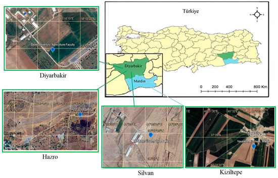
Figure 1.
Experimental areas. The locations of the experimental areas were selected in the provinces of Diyarbakir and Mardin in southeastern Türkiye. (detailed description can be found in the Section 2.1).
The saturation levels varied between locations: 66.00, 59.4, 72.00 and 65 in the Dicle University experimental area, Kiziltepe, Silvan and Hazro, respectively. The Mardin and Dicle University experimental areas had the highest lime ratios (19.14% and 11.40%, respectively). The pH values of experimental soils were >7.19. The organic matter content of Dicle University experimental soil was lower than that of the other locations. The highest altitude was in the Hazro location (1090 m.a.s.l). In contrast, the lowest altitude was in the Kiziltepe location (480 m.a.s.l) (Table 1).
The experiments were based on two factorial experimental designs with randomized blocks and four replications in each environment. In the experiments, four FLIP genotypes (FLIP97-254C, FLIP99-34C, FLIP98-143C and FLIP98-206C) obtained from ICARDA, five standard cultivars (Diyar-95, Arda, Azkan, Gokce and Cagatay) obtained from Türkiye, nine hybrids (D: Konya × Balikesir and R: Diyar-95 × ILC 482) and one local variety (N5-5) were used. The locations were determined as main plots and genotypes as sub-plots. The plots consisted of 5 m in length, six rows and 40 cm intervals. The seeds were sown in November 2015. The seeds were sown manually at a sowing density of 55 seeds/m2. Nitrogen (30 kg ha−1) and phosphorus (50 kg ha−1) fertilizers were applied. Data on seed yield were obtained from 6.4 m2 of each plot.
Climate Data for Experimental Areas
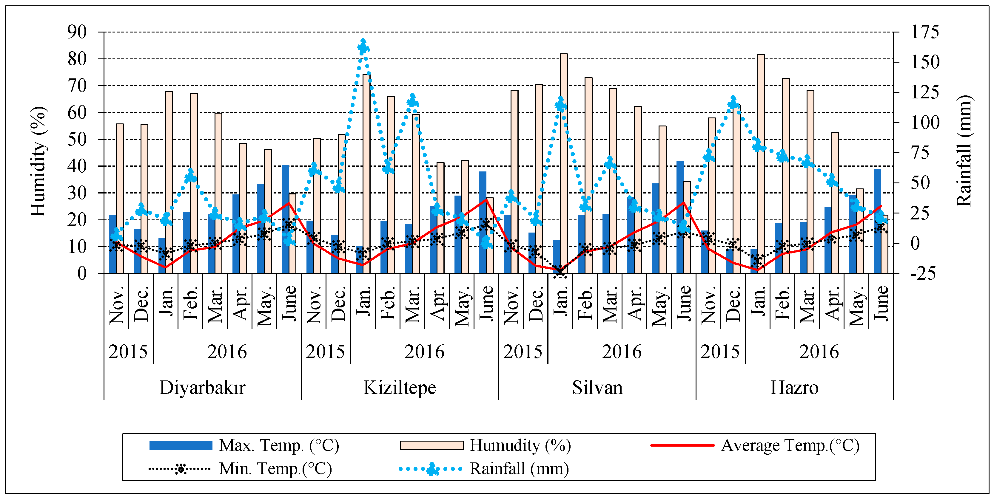
The climate data of locations during the experiment years are shown in Figure 2. The total rainfall of the Hazro (518.3 mm) and Kiziltepe (504.6 mm) locations was higher than Silvan (343.3 mm) and Diyarbakir (179.6 mm). The minimum average temperature between November and March was recorded in Silvan and Hazro. The maximum temperature in Kiziltepe and Hazro was lower than in Diyarbakir and Silvan from March to June. The average temperature in Kiziltepe and Diyarbakir was higher than in Hazro and Silvan from March to June. The Silvan location had higher relative humidity compared to other locations (Figure 2).
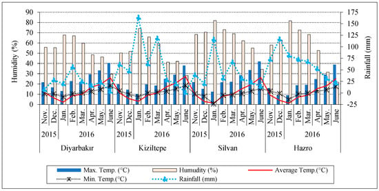
Figure 2.
Climate data for experimental environments.
2.2. Methods
2.2.1. Methodology of GGE Biplot
Data were subjected to GGE biplot analysis to determine the effect of location, genotype and location × genotype interaction for yield in Genstat 12th Edition (Version: 12.1.0.3338) software. The cluster analysis was realized to divide genotypes into groups based on similarity in yield using the Ward method (standardized by column) in JMP-Pro17 (Version: 17.0.0.622753) software. According to Gabriel [16] and Yan [8], the singular values were divided into genotype and environment scores before biplots were constructed to approximate the two-way data. The GGE biplot model was detailed by data scaling before singular value decomposition. Graph analysis of the GGE biplot was realized by single-value decomposition according to the report by Yang et al. [17]. It was used to visualize the data [18]. These centering methods were involved in the GGE biplot. The correlation between the two environments is shown in Equation (1)–(5), which explains the cosine of the angle between the vectors.
Pij = yij − μ − βj = αi + φij
Pij = yij= μ + βj + αi + φij
The symbols in the equations can be explained as follows:
f: the partitioning factor (0–1)
Yij: the mean of ith genotype in jth environment
μ: effect of the grand mean
ɑi: main effect of genotype
βj: main effect of environment
φij: specific genotype by environment interaction
sj: scaling factor (the standard error in environment)
j: removing heterogeneity among the environments
2.2.2. Methodology of AMMI Biplot
AMMI analysis was performed in Python 3 Google Compute Engine (https://colab.google/ (accessed on 10 October 2024)) on a grouping basis with the responses of the genotypes and environments taken together [13]. Gollob’s test was used to retain the multiplicative axis terms [19]. Axes (PCA1 and PCA2) were represented by genotype and environment variation (Equation (6)).
Yij: The observed performance (e.g., yield) of the i-th genotype in the j-th environment,
μ: The grand mean across all genotypes and environments,
Gi: The additive effect of the i-th genotype (genotypic main effect),
Ej: The additive effect of the jjj-th environment (environmental main effect),
λk: The singular value for the k-th principal component,
γik: The score of genotypes i on the k-th principal component,
δjk: The score of environment j on the k-th principal component,
t: The number of significant IPCAs retained in the model (based on statistical tests like Gollob’s F-test or cross-validation),
eij: The residual error term.
2.2.3. Architecture of Fuzzy C-Means Clustering
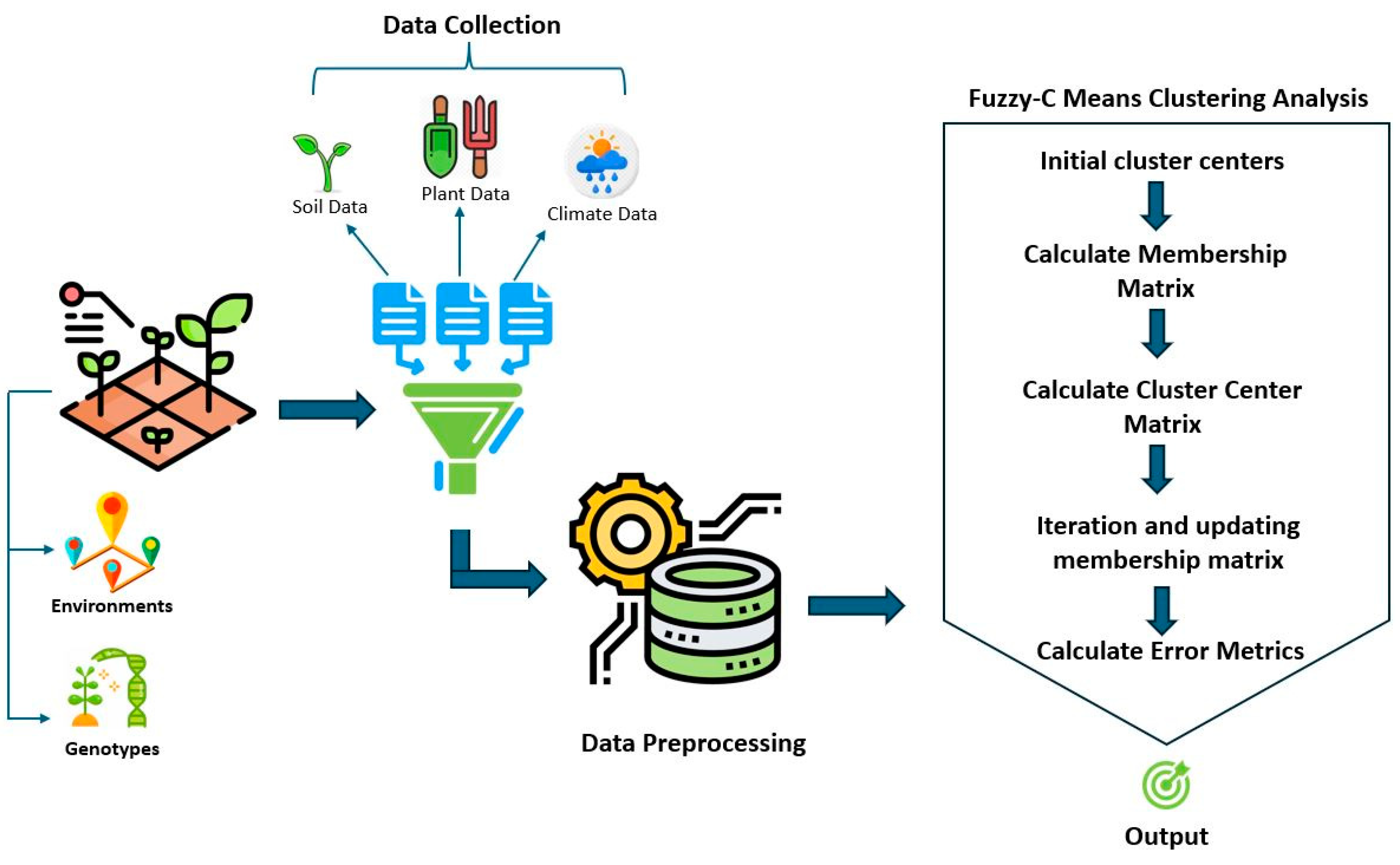
Fuzzy C-means clustering was used to divide the multivariate dataset of chickpea lines tested in different collections into a collection of c clusters and associate the data with more than one cluster (Equation (3)) [14,20]. The flowchart of the fuzzy C-means clustering analysis is given in Figure 3.
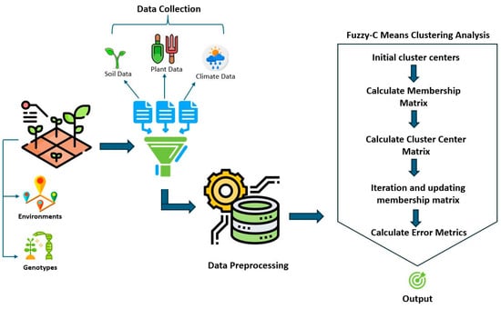
Figure 3.
Flowchart of evaluation of environment–genotype and climate data by fuzzy C-means cluster analysis.
In the clustering analysis performed with the yield values obtained from chickpea lines grown in different locations, FPC, D-B Index, Dunn Index, Silhouette Score, RMSE and Partition Entropy error metrics were used to evaluate the success and accuracy of the clustering algorithm and reveal how the genotypes performed according to different cluster numbers. The methodology for these metrics is represented below (Equation (7)–(9)).
The degree of membership uij and the cluster centers cj are updated iteratively as follows:
N: Total number of data points,
C: Total number of clusters,
xi: The i-th data point,
cj: The centroid of cluster j,
uij: Membership degree of the i-th data point in the j-th cluster,
m: Fuzziness parameter (degree of fuzziness),
∥xi−cj∥2: Squared Euclidean distance between xi and cj
ck: The centroid of cluster k, used to compare distances between data points (xi) and different cluster centers.
Fuzzy Partition Coefficient (FPC)
FPC analysis was used to understand how well divided the dataset was obtained from chickpea lines tested in different locations, in addition to evaluating the quality of clustering to learn the clarity of clusters (Equation (10)). The higher the FPC value obtained as a result of this analysis, the clearer the boundaries between clusters, and the more likely each data point belongs to only one cluster [14]. In the equation, the sum of the square of the degree of cluster membership of the yield obtained from each location provided the determination of the clustering quality [20].
N: Number of data points
C: Number of clusters
uik: The degree to which data point i belongs to cluster k
Davies–Bouldin Index (D-B Index)
The D-B Index was used to measure the similarity between clusters obtained from chickpea lines tested at different locations and the frequency within clusters. A low D-B Index indicated that the separation between clusters was good, and data points within clusters were close to each other [21]. The equation measured the total segregation by taking into account the spread of each cluster and its distance from other clusters (Equation (11)).
C: Number of clusters
Si: Average distance indicating the spread of data within the cluster
dij: Distance between cluster centers
Sj: The intra-cluster scatter (compactness) for cluster j
Dunn Index
The Dunn Index was used to calculate the ratio between the minimum distance between the clusters and the maximum distance within the clusters formed from the obtained data of chickpea lines tested at different locations. A higher Dunn Index indicated that the separation between clusters was more pronounced, and the data within clusters were closer [20]. The equation revealed the quality of clustering by comparing the distance between clusters with the distance within clusters (Equation (12)).
d(i, j): Distance between cluster centers i and j
k: Maximum distance in cluster k
c: Number of clusters
Silhouette Score
The Silhouette Score was used to understand the fit of the data point obtained from each location to its cluster and its difference from other clusters. A score close to 1 indicated that the data points fit well into their clusters, and the distinction between clusters was clear [22] (Equation (13)).
a(i): Average distance of data point i from other data points in its cluster
b(i): Average distance from data point i to points in the nearest other cluster
Root Mean Square Error (RMSE)
RMSE tested the error level of the clustering model created from the data obtained from each location. A low RMSE value explained that the distance of the data points to the cluster center was small. A low RMSE value indicated better clustering [14]. The equation calculated the mean squared distance of all data points to the cluster center (Equation (14)).
xi: Actual data point
Predicted value as a result of clustering
n: Total number of data points
Partition Entropy (PE)
PE calculated the uncertainty of the clusters formed from the data obtained from each location. A high value of Partition Entropy indicated that the clusters were ambiguous, and the clustering results were not accurate, evaluating the probability that the data obtained from the locations belonged to more than one cluster [14]. The equation measured uncertainty by taking the entropy of the belonging degree of the location dataset to different clusters (Equation (15)).
N: Number of data points,
C: Number of clusters,
uiJ: Membership degree of the i-th data point in the j-th cluster.
2.2.4. Statistical Analysis
The GGE biplots were used to obtain the relationship between genotypes and environments using polygon, ranking and comparison techniques [8]. Data standardization was performed in GGE biplot analysis. GGE biplot allowed each of the models (Equations (1)–(5)) to be scaled in different techniques. The analysis of variance and averages of genotypes was performed using JMP Pro17 statistical analysis software. The fuzzy C-means clustering model and AMMI analysis was coded in Python using Google Colab Notebook. The coding was performed using a computer with a 13th generation 7 processor, 32 GB RAM and NVIDIA GeForce RTX 4060 chip. The dataset was uploaded as a csv file to Google Colab Notebook and the coding process started. In Python, Skyfuzzy was used to build the model, NumPy for numerical calculations [23], Pandas for data analysis [24] and Matplotlib for data visualization.
3. Results
3.1. Analysis of Variance
Nineteen chickpea genotypes were examined in four different locations to evaluate yield performance. Variance analysis results are given in Table 2, and G×E mean values are given in Table 3.

Table 2.
Analysis of variance for yield performances of chickpea genotypes.

Table 3.
Experiment means for the yield of 19 genotypes at four locations during the 2016 growing season.
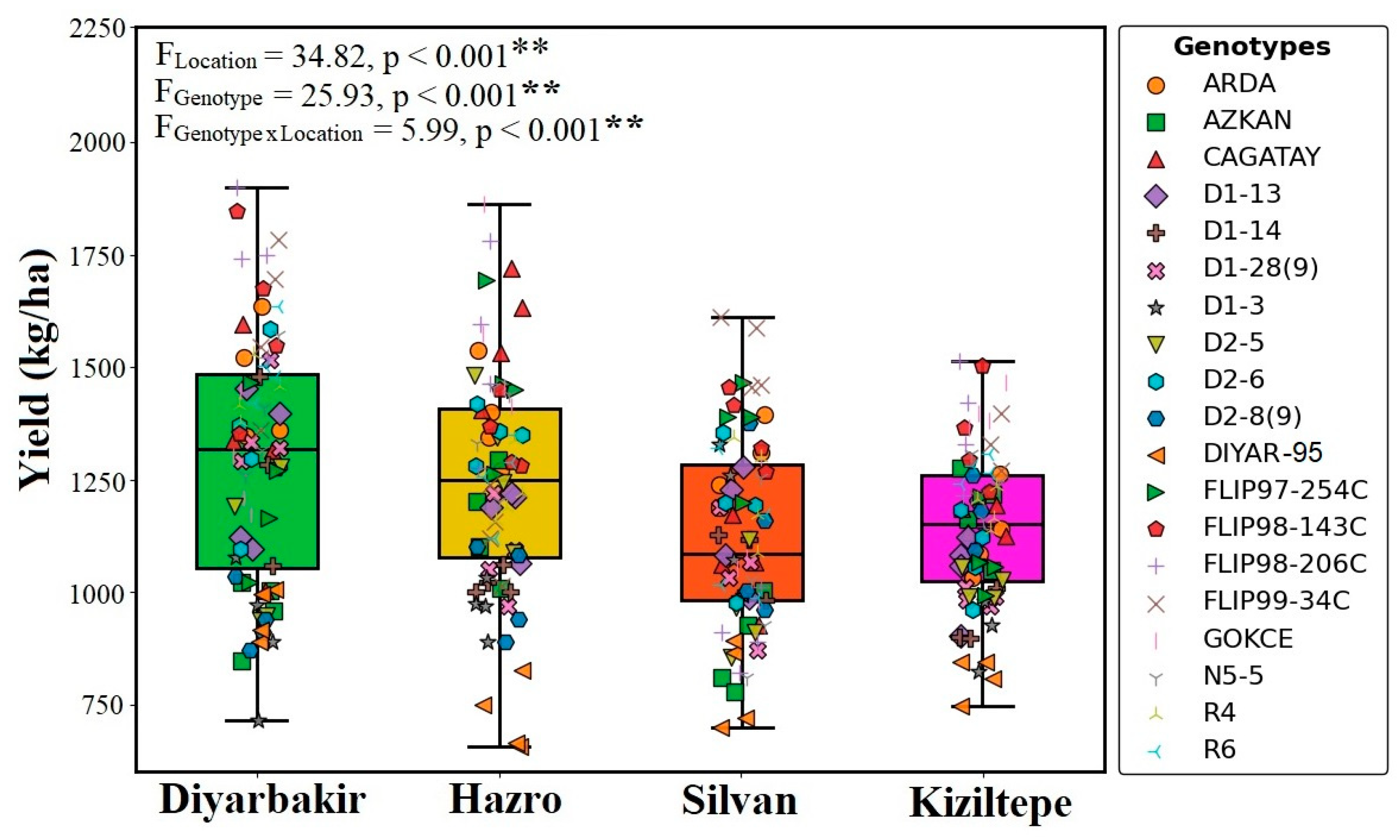
The highest seed yield was obtained from the FLIP98-206C (1727.3 kg ha−1) genotype in the Diyarbakir location. The Diyar-95 cultivar had the lowest seed yield (723.5 kg ha−1) in the Hazro location. Among all genotypes, FLIP98-143C had the highest seed yield (1415.5 kg ha−1), while the Diyar-95 cultivar exhibited the lowest performance (Table 3; Figure 4).

Figure 4.
Effect of different locations and genotypes on chickpea yield (**: p ≤ 0.001 significant level).
3.2. Comparison of Environments Based on Discriminating Ability
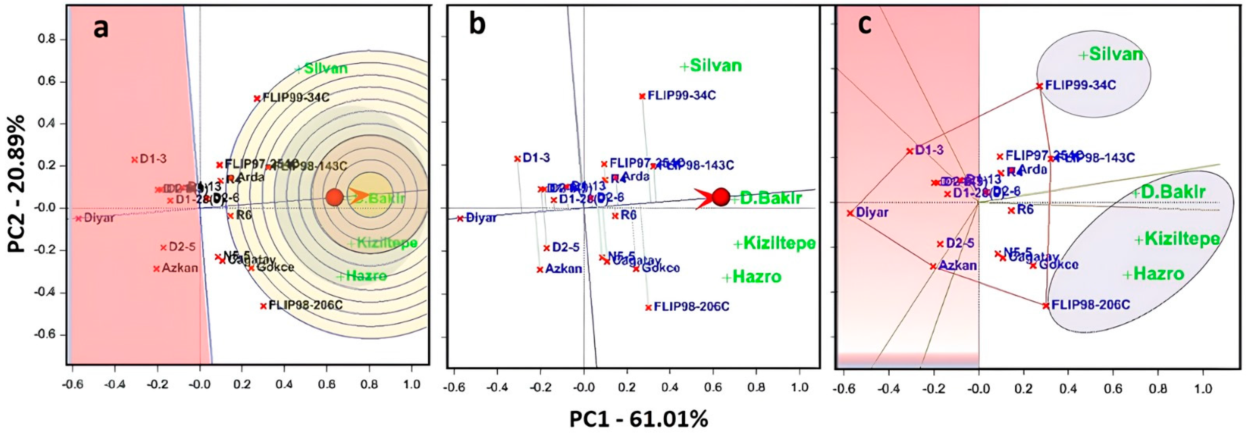
In the study, the interpretation of the biplots was based on data presented in Table 2, and the GGE biplots were obtained from comparison, ranking and polygon techniques. Figure 5 describes an ideal genotype, which could be called the center of the concentric circles, and points on the AEA or AEC in the positive direction.

Figure 5.
Here, (a) the comparison biplot graph shows the distance of genotypes to the ideal center. Genotypes were ranked by mean and stability. Average Environment Axis (AEA) ranked the mean performance and stability of genotypes across environments. (b) GGE biplot ranking graph shows the stability of genotypes for the mean of seed yield. Average Environment Coordination (AEC: red circle) ranks the mean performance of genotypes. (c) Polygons show suitable genotypes in each environment and which genotype won where.
According to the results, PC1 and PC2 explained 81.90% of the total variation of the environment-centered G×E. The ideal genotype was equal to the longest vector on the positive side of the AEA, and this vector indicated the highest average yield among the other genotypes (Figure 5a). Genotypes that were located closer to the ideal genotype could be preferred to other genotypes. Therefore, FLIPP98-206C and FLIPP99-34C genotypes were more desirable. However, genotypes located closer to these genotypes could be more desirable than other genotypes. Diyar-95 was the highest stable genotype. However, this case does not mean Diyar-95 was good. This case could be explained by that the relative performance of the Diyar-95 cultivar was consistent. As a matter of fact, D1-3 and Azkan genotypes, which were located closer to the Diyar-95 cultivar, were very poor and variable. However, the least stable genotype was the Diyar-95 cultivar because D1-3 and Azkan genotypes showed reasonable yield in the examined environments. In the graph, the Diyarbakir location was the most representative compared to other locations. The Diyarbakir location was a good test environment for selecting adapted genotypes. The ideal test environment was the most representative point on the AEA in the positive direction and equals the longest vector of all environments on the origin. Therefore, the Diyarbakir location was the closest to this point and was the best environment. However, the Silvan location was the poorest environment for selecting genotypes adapted to all regions. Additionally, Kiziltepe and Hazro locations, which were in the center of the concentric circles, had high performance in FLIPP98-206C and FLIPP98-143C (Figure 5a).
3.3. Ranking Performance of Genotypes in Environments
Genotypes were ranked to evaluate performance in different environments and defined the average-environment coordination view of the GGE biplot (Figure 5b). The single-arrowed line was the AEC or AEA abscissa, which indicates a higher mean yield among environments. FLIP98-206C and FIP99-34C genotypes had the highest yield, and the lowest yield was in the Diyar-95 cultivar in the Diyarbakir location. The dual-arrowed line was the AEC ordinate, and this indicated poorer stability and higher variability in either direction. Diyar-95 had lower than expected yield in all environments, and thus, it was the most unstable cultivar among other genotypes. In contrast, FLIPP98-206C and FLIPP99-34C genotypes had higher than expected yields in all environments, especially the Diyarbakir location (Figure 5b).
3.4. Detection of the Best Which-Won-Where Performance of Genotypes
GGE biplot analysis explained that the genotypes placed at the corners of the polygon were the best or the poorest in the studied environments. Accordingly, the equality line between D1-3 and FLIPP99-34C showed that FLIPP99-34C was better at the Silvan location. The line of equality between D1-3 and FLIPP99-34C showed that FLIPP99-34C was better than D1-3 at all locations. However, FLIPP98-143C was located on the line connecting D1-3 and FLIPP99-34C, and FLIPP98-143C also had high performance after FLIPP99-34C at the Silvan location. Moreover, the line of equality between FLIPP98-143C and FLIPP98-206C showed that FLIPP98-206C was better in the Diyarbakir (Center), Kiziltepe and Hazro locations. FLIPP99-34C came first in the Silvan location and FLIPP98-206C in other locations. These genotypes should be selected in the winning locations with this pattern. Genotypes on the left of the coordinate plane (red background) did not stand out in any of these locations (Figure 5c).
3.5. AMMI Biplot
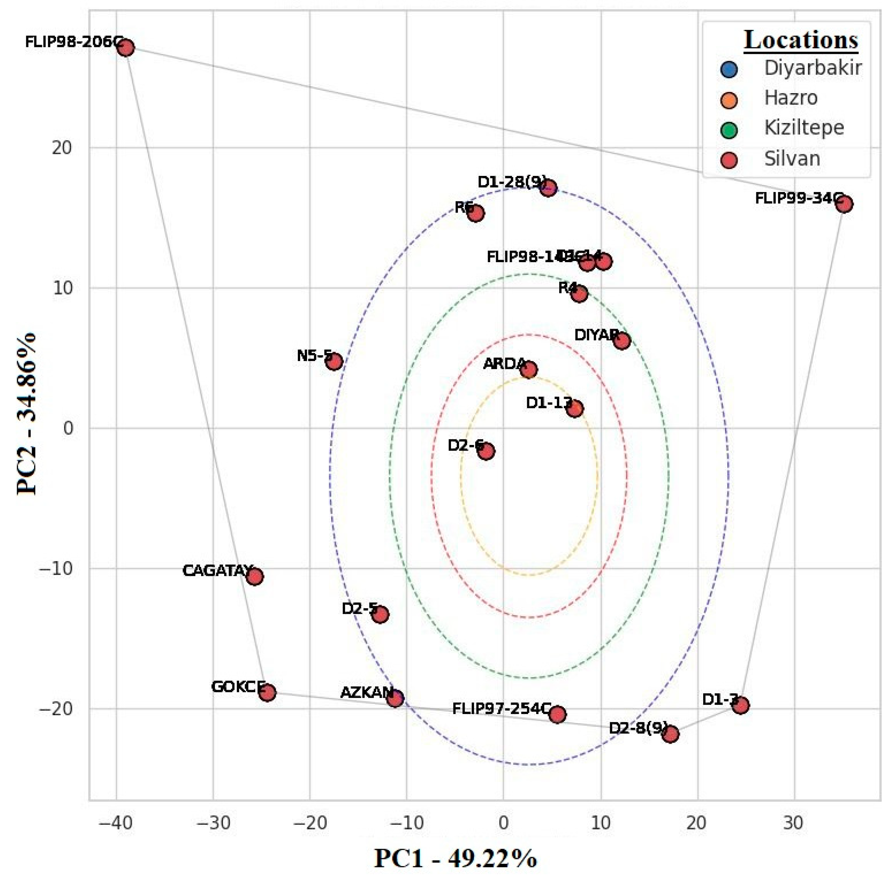
The AMMI biplot explained the performance and environmental adaptability of the genotypes at each location. The PC1 and PC2 axes used in the AMMI biplot showed the response of the genotypes to environmental effects. The PC1 axis explained 49.22% of the total variation, and the PC2 axis explained 34.86% (Figure 6). In total, these two components explained 84% of genotype–environment interactions, indicating the biplot adequately represented genotype performance and environmental interactions [13] (Table 4).
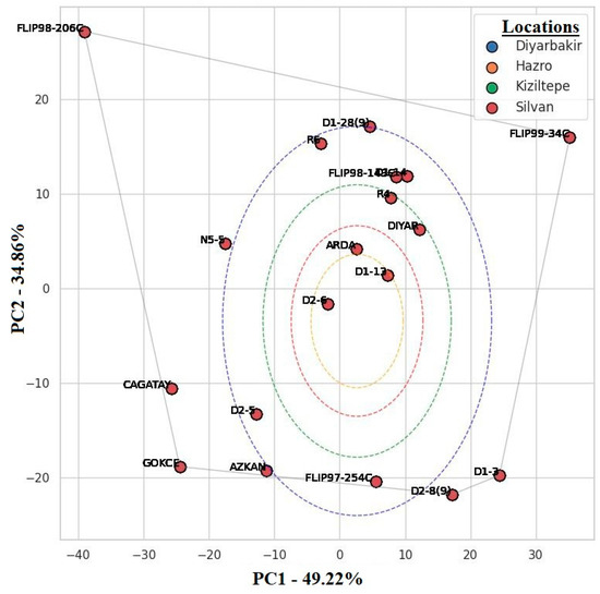
Figure 6.
AMMI biplot of yield stability and GxE interactions of different locations and genotypes.

Table 4.
Effects of different sources of variation on total variability: percentages of variance explained by genotype, environment and genotype × environment interactions with the AMMI model.
The genotypes FLIP98-206C and FLIP99-34C were situated at the extremes of the AMMI biplot. FLIP98-206C showed high yield potential especially in the Diyarbakir location, indicating that this genotype had high adaptability to the environmental conditions (e.g., soil structure, climate) specific to this location [6,18]. D1-12, ARDA and D2, which were located closer to the center of the biplot, were more stable compared to other genotypes and had a high ability to adapt to different environmental conditions. The narrow distribution of chickpea genotypes in the Silvan and Hazro locations and the wide distribution in the Kiziltepe location indicated that the effect of environmental factors on genotypes might be variable. The fact that D1-12 and ARDA genotypes were prominent in Silvan and Hazro and R6 and D1-28 genotypes were prominent in Kiziltepe in terms of yield indicates that these genotypes were better adapted to the environmental conditions of these locations (Figure 6).
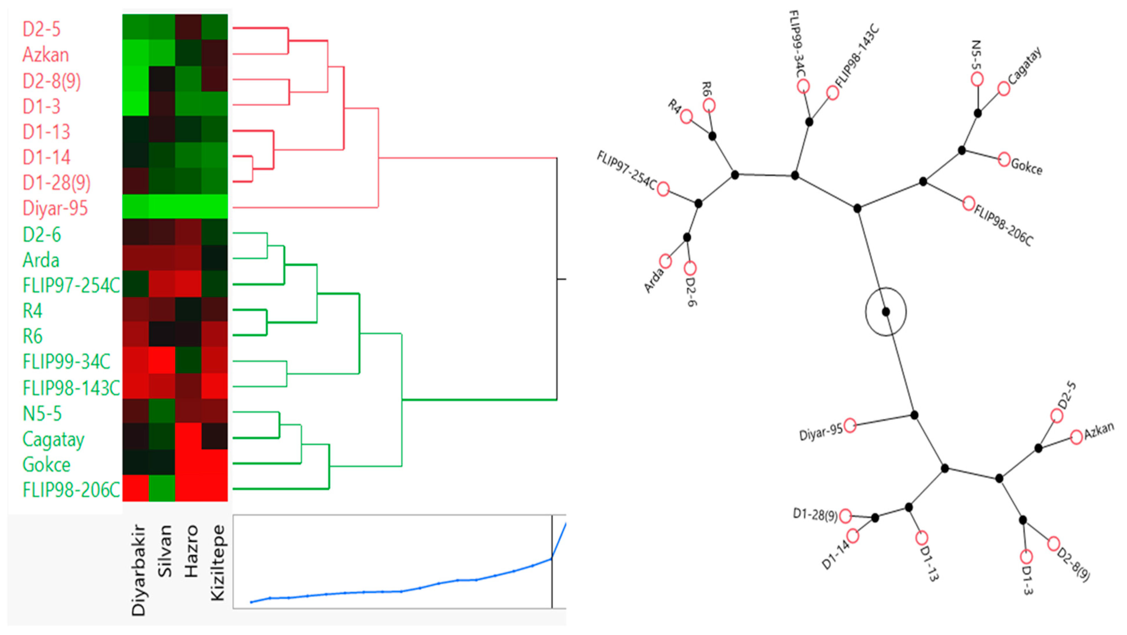
3.6. Ward’s Method Clustering
Chickpea genotypes were classified by cluster analysis depending on Ward’s method, using standard data (Figure 7). The main aim of cluster analysis was to detect the genetic distance of genotypes from each other. To prevent time loss in studies with many genotypes, genotypes can be categorized by cluster analysis, and some genotypes can be selected from fakes in distant clusters. In this analysis, the grouping of genotypes was realized by Ward’s method using Euclidean distance based on the standardized mean of yield, and the Euclidean distance of 19 genotypes was classified into two groups. The first cluster contained genotypes D2-5, Azkan, D2-8(9), D1-3, D1-13, D1-14, D1-28(9) and Diyar-95. These genotypes had similarities and low values for seed yield. The second cluster contained genotypes D2-6, Arda, FLIP97-254C, R4, R6, FLIP99-34C, FLIP98-143C, N5-5, Cagatay, Gokce and FLIP98-206C. These genotypes had similarities and high values for seed yield. Genotypes D2-6, Arda and FLIP97-254C had similar yield performance in the Hazro location. Genotypes R4, R6, FLIP99-34C and FLIP98-143C had similar yield performance in the Diyarbakir location. Genotypes Cagatay, Gokce and FLIP98-206C had similar high-yield performance in the Hazro location. Between the two clusters, the second group was more suitable for seed yield performance in the selection of genotypes (Figure 7).

Figure 7.
Dendrogram of the cluster analysis of 19 chickpea genotypes based on yield under locations using Ward’s method.
3.7. Fuzzy C-Means Clustering
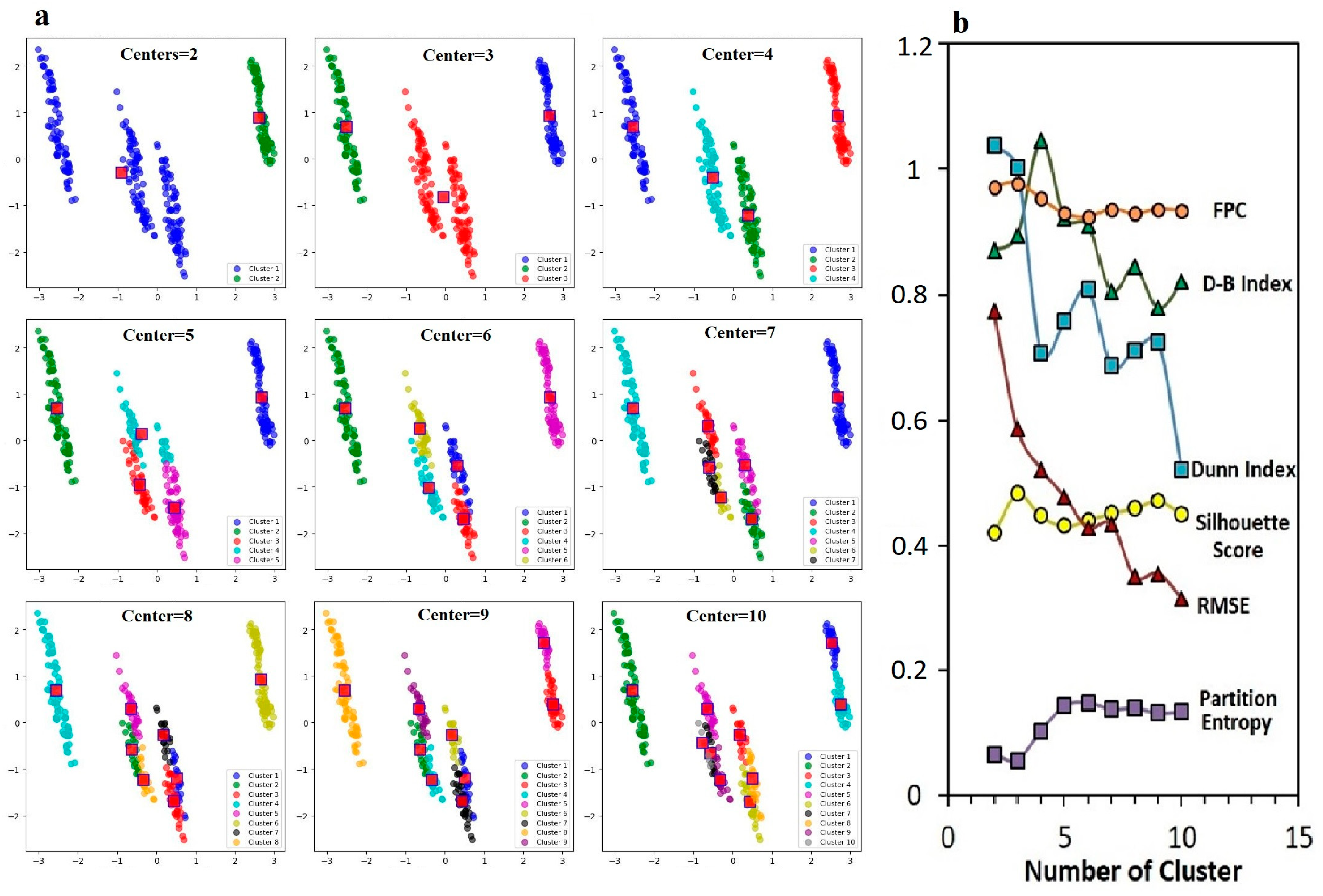
The distribution of the analyses performed for the fuzzy C-means (FCM) clustering method at different cluster numbers (from 2 to 10) was shown by visualizing the Principal Component Analysis (PCA) components. Each box represented a specific number of clusters (Centers = 2). Increasing the number of clusters indicated that genotypes were further categorized (Figure 8a). In addition, the values of the quality measured (FPC, D-B Index, Dunn Index, Silhouette Score, RMSE, Partition Entropy) for different cluster numbers used in the fuzzy C-means (FCM) clustering method are shown (Figure 8b).
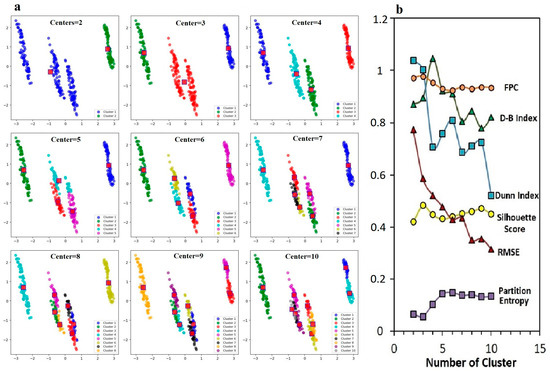
Figure 8.
Effect of different cluster numbers on fuzzy C-means clustering performance (a), comparative analysis of error metrics (b): Silhouette Score, Dunn Index, Partition Entropy, RMSE, FPC and Davies–Bouldin Index.
For the purposes of the research, the FPC value was between two and five clusters, which was quite high. This showed that the genotypes were clearly separated in the number of clusters. The D-B Index, which showed the similarity between clusters and the cohesion within clusters, was divided into five clusters, which showed that the clusters were best separated from each other. The Dunn Index, which showed the minimum distance between clusters and the maximum diameter ratio within clusters, was obtained as four and five clusters, and these cluster numbers were appropriately effective in grouping the genotypes. The Silhouette Score was higher, especially between three and five clusters. The RMSE value started to decrease after six clusters, indicating that the errors decreased with more clusters. The Partition Entropy value increased as the number of clusters increased, which indicated more clusters introduced uncertainty. When the FPC and Dunn Index were high together (e.g., in the range of 3–6 clusters), clusters were clearly separated, and the distance between clusters was quite large. This suggested that the optimal number of clusters for separating genotypes into distinct groups was four or five. When the Silhouette Score was high and the D-B Index was low, the separation between clusters became quite clear. As the RMSE value decreased, the clustering accuracy increased, whereas the increase in Partition Entropy brought uncertainties with the increasing number of clusters.
4. Discussion
In this study, the usability of GGE biplots, AMMI biplots, clustering and fuzzy logic methods in revealing the performance of chickpea genotypes tested at different locations and determining superior genotypes was investigated. In the biplot analysis, the genotype–environment (G×E) interactions, performance and stability of genotypes in different environments were determined. Yousefabadi et al. [25] reported that the GGE biplot method can be used effectively to determine suitable genotypes with concepts such as “ideal genotype” and “ideal environment” and measure the representativeness of environments [26]. In our study, FLIPP98-206C and FLIPP99-34C genotypes showed high yield and stability at the Diyarbakir location (Figure 5a–c). The fact that FLIPP98-206C and FLIPP99-34C differed between locations in biplot analysis and stood out at the Diyarbakir location indicates that environmental factors affect the performance of these genotypes [27,28]. As a matter of fact, Rahmati et al. [29] also reported that the performance of genotypes can vary depending on the location, and the performance of genotypes in similar environments is similar, but in different environments, the performance is different. This shows that the GGE biplot gives successful results in mega-environmental analysis [30]. However, although GGE biplot analysis is a powerful tool for understanding genotype–environment interactions, the method has some limitations. While this method is effective in visualizing genotype performance and identifying ideal genotypes and environments, it ignores environmental effects.
By excluding environmental effects from the model, it focuses only on the visualization of genotypes and G×E interactions, which in some cases limits the detailed analysis of environmental effects [29]. Furthermore, analysis of the first two principal components (PC1 and PC2), which explain most of the variation in the data, may not adequately reflect the complex interactions of genotypes and environments. Therefore, the integration of other statistical methods (such as AMMI or WAASB) may offer a more comprehensive assessment of genotype–environment main lines, according to Asadi et al. [26] and Rahmati et al. [29]. For this purpose, in addition to biplot analysis, the AMMI (additive main effects and multiplicative interaction) model was also used in our study (Figure 1). The AMMI model, which analyzes genotype–environment (G×E) interactions in detail, facilitates the process of identifying genotypes with high yield potential by revealing the adaptability of genotypes to the environment [26,29,31]. In our study, PC1 and PC2 axes explained 84% of the total variation (Figure 6). This indicated that the AMMI model was successful in representing the performance of genotypes in the face of environmental effects. Rahmati et al. [29] also reported that genotypes with high yield under different environmental conditions can be identified by AMMI analysis, and it can be an effective model for evaluating the results, especially in breeding programs. Similarly, Asadi et al. [26] reported that the use of the AMMI model as a graphical tool in the stability analysis of genotypes provides a visual evaluation of genotype–environment relationships.
The results obtained in our study showed that most of the variation in the performance of genotypes was due to environmental effects, but G×E interactions also played a significant role. As a matter of fact, environmental differences such as climate, altitude, soil characteristics, etc., between the locations where the research was conducted were reflected in the performance of the genotypes. FLIP98-206C showed high yield potential especially in the Diyarbakir location, indicating that this genotype has high adaptability to the environmental conditions (such as soil structure and climate) specific to this location [6,18]. The fact that chickpea genotypes were narrowly distributed in Silvan and Hazro locations and widely distributed in the Kiziltepe location indicates that the effect of environmental factors on genotypes may be variable. In terms of yield, D1-12 and Arda genotypes in Silvan and Hazro and R6 and D1-28 genotypes in Kiziltepe indicate that these genotypes are better adapted to the environmental conditions of these locations (Figure 6). This finding suggests that environmental characteristics should be taken into account to optimize the superior performance of genotypes in specific environments [28]. The AMMI biplot provides a strong foundation for stability and environmental adaptation by analyzing variance components in detail, but it can increase interpretation complexity. Consequently, we strengthened the interpretation of the research data with Ward method clustering and fuzzy C-means (FCM), which are successful in modeling uncertainty and identifying complex patterns. In our research, we determined the closeness and distance of genotypes in terms of the traits examined by Ward method clustering. In the clustering, genotypes were divided into two groups (Figure 7). In the first group, D2-5, Azkan, D2-8(9), D1-3, D1-13, D1-14, D1-28(9) and Diyar-95 genotypes were included, and these genotypes gave low values in terms of seed yield. In the second group, D2-6, Arda, FLIP97-254C, R4, R6, FLIP99-34C, FLIP98-143C, N5-5, Cagatay, Gökce and FLIP98-206C genotypes were included. All these genotypes had similarities in terms of the characteristics examined and showed high values in terms of seed yield.
Genotypes D2-6, Arda, FLIP97-254C, Cagatay, Gokce and FLIP98-206C had similar yield performance at the Hazro location, while genotypes R4, R6, FLIP99-34C and FLIP98-143C had similar yield performance at the Diyarbakir location (Figure 7). Ward’s method is an important tool for revealing genetic diversity in breeding studies, and there are studies on the usability of this method. Indeed, Mahmood et al. [32] grouped the genotypes by cluster analysis according to Ward’s method, identified the genotypes with superior performance and revealed genetic diversity. In this research, since the fuzzy C-means (FCM) method offers a wider range of applications compared to other methods with its ability to better manage uncertainty and its ability to identify complex patterns [33], we revealed the adaptation potential of chickpea genotypes to different environmental conditions with the multidimensional FCM method. By analyzing the responses of genotypes to environmental variability with the fuzzy C-means (FCM) clustering method, the performance between different cluster numbers was compared. In our study, FCM was successful in determining the adaptation of genotypes to different environmental conditions and provided optimal segregation, especially in four or five clusters (Figure 8). The Fuzzy Partition Coefficient (FPC) and Dunn Index showed that the cluster separation of genotypes was clearest in 4–5 clusters. This suggests that genotypes are best grouped in terms of both performance and stability [34]. The Silhouette Score confirms that the separation between clusters is clear, with particularly high values in clusters 3 to 5 [35]. Yang et al. [36]. reported that in modeling epistasis and genetic variation, FCM’s ability to manage uncertainty provides a better understanding of gene–gene interactions. While FCM better incorporates uncertainty into the model, new methods may be needed to further optimize decision mechanisms in more complex situations (e.g., in transition regions) [37].
This study shows that the FCM method is a powerful tool for analyzing the adaptation of genotypes to environmental variability. However, a more comprehensive analysis can be performed by integrating the results obtained with FCM with other methods such as the AMMI or GGE biplot.
5. Conclusions
The yield performance and environmental stability of different chickpea genotypes were successfully evaluated using the GGE biplot, AMMI analysis and fuzzy C-means clustering methods. In the study, the GGE biplot, AMMI analysis and fuzzy C-means clustering analysis showed that the Diyarbakir location was a suitable test environment for genotypes with high yield and stable performance. Especially FLIP98-206C and FLIP99-34C genotypes were identified as having high yield potential in all test sites. On the other hand, the Diyar-95 cultivar showed low and unstable performance. The fuzzy C-means clustering method based on machine learning and artificial intelligence used in the study increased the accuracy of yield predictions. However, the combined use of the GGE biplot, AMMI analysis and fuzzy C-means clustering methods offered different perspectives in detecting G×E interaction. In the future, integrating these methods with different machine learning algorithms will provide more efficient and automated decision support systems in plant breeding. The integration of these methods in large datasets and environmental conditions is expected to provide effective results in determining the environmental adaptation and potential of genetic materials.
Supplementary Materials
The following supporting information can be downloaded at: https://www.mdpi.com/article/10.3390/agronomy15020300/s1.
Author Contributions
Conceptualization, M.T. and M.Y.; Methodology, M.T. and B.T.B.; Software, M.Y.; Validation, L.Y. and B.T.B.; Formal analysis, M.T. and S.I.; Investigation, M.Y. and L.Y.; Data curation, S.B.R., S.I. and L.Y.; Writing—original draft, M.T., S.B.R. and S.I.; Writing—review & editing, M.T., S.B.R., M.Y., L.Y. and B.T.B.; Visualization, S.I.; Supervision, M.T. and B.T.B. All authors have read and agreed to the published version of the manuscript.
Funding
This research received no external funding.
Data Availability Statement
Data is contained within the article and Supplementary Material.
Conflicts of Interest
The authors declared that they have no conflicts of interest.
References
- Jendoubi, W.; Bouhadida, M.; Boukteb, A.; Béji, M.; Kharrat, M. Fusarium wilt affecting chickpea crop. Agriculture 2017, 7, 23. [Google Scholar] [CrossRef]
- Ipekesen, S.; Basdemir, F.; Tunc, M.; Bicer, B.T. Minerals, vitamins, protein and amino acids in wild Cicer species and pure line chickpea genotypes selected from a local population. J. Elem. 2022, 27, 127–140. [Google Scholar] [CrossRef]
- FAOSTAT. 2022. Available online: https://www.fao.org/faostat/en/#data/QCL (accessed on 10 October 2024).
- Shah, T.M.; Imran, M.; Atta, B.M.; Ashraf, M.Y.; Hameed, A.; Waqar, I.; Shafiq, M.; Hussain, K.; Naveed, M.; Aslam, M.; et al. Selection and screening of drought tolerant high yielding chickpea genotypes based on physio-biochemical indices and multi-environmental yield trials. BMC Plant Biol. 2020, 20, 171. [Google Scholar] [CrossRef] [PubMed]
- Padi, F.K. The relationship between stress tolerance and grain yield stability in cowpea. J. Agri. Sci. Camb. 2007, 142, 431–444. [Google Scholar] [CrossRef]
- Ebdon, J.S.; Gauch, H.G. Additive main effect and multiplicative interaction analysis of national turfgrass performance trials: I. Interpretation of genotype 3 environment interaction. Crop Sci. 2002, 42, 489–496. [Google Scholar] [CrossRef]
- Sabaghnia, N.; Dehghani, H.; Sabaghpour, S.H. Nonparametric methods for interpreting genotype× environment interaction of lentil genotypes. Crop Sci. 2006, 46, 1100–1106. [Google Scholar] [CrossRef]
- Yan, W. Singular-value partitioning in biplot analysis of multi-environment trial data. Agron. J. 2002, 94, 990–996. [Google Scholar] [CrossRef]
- Gower, J.C. Multivariate analysis and multivariate geometry. Statistician 1967, 17, 13–28. [Google Scholar] [CrossRef]
- Mungomery, V.E.; Shorter, R.; Byth, D.E. Genotype × environment interactions and environment adaptation. I. Pattern analysis—Application to soya bean populations. Aust. J. Agric. Res. 1974, 25, 59–72. [Google Scholar] [CrossRef]
- Gauch, H.G.; Zobel, R.W. Predictive and postdictive success of statistical analyses of yield trials. Theor. Appl. Genet. 1988, 76, 1–10. [Google Scholar] [CrossRef] [PubMed]
- Ambuel, J.R.; Colvin, T.S.; Karlen, D.L. A fuzzy logic yield simulator for prescription farming. Trans. ASAE 1994, 37, 1999–2009. [Google Scholar] [CrossRef]
- Gauch, G. Statistical Analysis of Regional Yield Trials: AMMI Analysis of Factorial Designs; Elsevier Science Publishers: Amsterdam, The Netherlands, 1992. [Google Scholar] [CrossRef]
- Bezdek, J. Pattern Recognition with Fuzzy Objective Function Algorithms; Plenum Press: New York, NY, USA, 1981. [Google Scholar] [CrossRef]
- Jelacic, M. Unsupervised Learning for Plant Recognition. Master’s Thesis, School of Information Science, Computer and Electrical Engineering, Halmstad University, Halmstad, Sweden, 2006. [Google Scholar]
- Gabriel, K.R. Le biplot: Outil d’exploration de données multidimensionnelles [Biplot—Tool for exploration of data]. J. Société Française Stat. 2002, 143, 5–55. [Google Scholar]
- Yang, C.H.; Chuang, L.Y.; Lin, Y.D. Epistasis analysis using an improved fuzzy C-means-based entropy approach. IEEE Trans. Fuzzy Syst. 2019, 28, 718–730. [Google Scholar] [CrossRef]
- Yan, W.; Tinker, N.A. Biplot analysis of multi-environment trial data: Principles and applications. Can. J. Plant Sci. 2006, 86, 623–645. [Google Scholar] [CrossRef]
- Gollob, H.F. A Statistical Model Which Combines Features of Factor Analytic and Analysis of Variance Techniques. Psychometrika 1968, 33, 73–115. [Google Scholar] [CrossRef]
- Dunn, J.C. A Fuzzy Relative of the ISODATA Process and Its Use in Detecting Compact Well-Separated Clusters. J. Cybern. 1973, 3, 32–57. [Google Scholar] [CrossRef]
- Davies, D.L.; Bouldin, D.W. A Cluster Separation Measure. IEEE Trans. Pattern Anal. Mach. Intell. 1979, 1, 224–227. [Google Scholar] [CrossRef] [PubMed]
- Rousseeuw, P.J. Silhouettes: A Graphical Aid to the Interpretation and Validation of Cluster Analysis. J. Comput. Appl. Math. 1987, 20, 53–65. [Google Scholar] [CrossRef]
- van der Walt, S.; Colbert, S.C.; Varoquaux, G. The NumPy Array: A Structure for Efficient Numerical Computation. Comput. Sci. Eng. 2011, 13, 22–30. [Google Scholar] [CrossRef]
- McKinney, W. Data Structures for Statistical Computing in Python. In Proceedings of the 9th Python in Science Conference, Austin, TX, USA, 28 June–3 July 2010. [Google Scholar] [CrossRef]
- Yousefabadi, V.A.; Mehdikhani, P.; Nadali, F.; Sharifi, M.; Azizi, H.; Ahmadi, M.; Fasahat, P. Evaluation of yield and stability of sugar beet (beta vulgaris L.) genotypes using GGE biplot and AMMI analysis. Sci. Rep. 2024, 14, 27384. [Google Scholar] [CrossRef] [PubMed]
- Asadi, B.; Shobeiri, S.S.; Asadi, A.A. Investigating of the Genotype× Environment Interaction Effect for Grain Yield in Red Bean Genotypes Using AMMI and GGE Biplot Methods. J. Crop Breed. 2024, 16, 86–102. [Google Scholar] [CrossRef]
- Supriadi, D.; Bimantara, Y.M.; Zendrato, Y.M.; Widaryanto, E.; Kuswanto, K.; Waluyo, B. Assessment of genotype by environment and yield performance of tropical maize hybrids using stability statistics and graphical biplots. PeerJ 2024, 12, e18624. [Google Scholar] [CrossRef] [PubMed]
- Daemo, B.B.; Ashango, Z. Application of AMMI and GGE biplot for genotype by environment interaction and yield stability analysis in potato genotypes grown in Dawuro zone, Ethiopia. J. Agric. Food Res. 2024, 18, 101287. [Google Scholar] [CrossRef]
- Rahmati, S.; Azizi-Nezhad, R.; Pour-Aboughadareh, A.; Etminan, A.; Shooshtari, L. Analysis of genotype-by-environment interaction effect in barley genotypes using AMMI and GGE biplot methods. Heliyon 2024, 10, e38131. [Google Scholar] [CrossRef] [PubMed]
- Vinu, V.; Alarmelu, S.; Elayaraja, K.; Appunu, C.; Hemaprabha, G.; Parthiban, S.; Shanmugasundaram, K.; Rajamadhan, R.; Saravanan, K.G.; Kathiravan, S.; et al. Multi-environment Analysis of Yield and Quality Traits in Sugarcane (Saccharum sp.) through AMMI and GGE Biplot Analysis. Sugar Tech. 2024, 1–19. [Google Scholar] [CrossRef]
- Demelash, H. Genotype by environment interaction, AMMI, GGE biplot, and mega environment analysis of elite Sorghum bicolor (L.) Moench genotypes in humid lowland areas of Ethiopia. Heliyon 2024, 10, e26528. [Google Scholar] [CrossRef]
- Mahmood, M.T.; Akhtar, M.; Cheema, K.L.; Ghaffar, A.; Ali, I.; Khalid, M.J.; Ali, Z. Genetic studies for detection of most diverse and high yielding genotypes among chickpea (Cicer arientinum L.) germplasm. Pak. J. Agric. Res. 2022, 35, 115. [Google Scholar] [CrossRef]
- Bezdek, J.C.; Ehrlich, R.; Full, W. FCM: The fuzzy c-means clustering algorithm. Comput. Geosci. 1984, 10, 191–203. [Google Scholar] [CrossRef]
- Cardoso, D.B.O.; Oliveira, L.F.; de Souza, G.S.; Garcia, M.F.; Medeiros, L.A.; Faria, P.N.; Cruz, C.D.; de Sousa, L.B. Using fuzzy logic to select coloured-fibre cotton genotypes based on adaptability and yield stability. Acta Scientiarum. Agron. 2021, 43, e50530. [Google Scholar] [CrossRef]
- Carneiro, V.Q.; Mencalha, J.; Sant’anna, I.d.C.; Silva, G.N.; Miguel, J.A.d.C.; Carneiro, P.C.S.; Nascimento, M.; Cruz, C.D. A novel fuzzy approach to identify the phenotypic adaptability of common bean lines. Acta Scientiarum. Agron. 2023, 45, e59854. [Google Scholar] [CrossRef]
- Yang, C.H.; Chuang, L.Y.; Lin, Y.D. An improved fuzzy set-based multifactor dimensionality reduction for detecting epistasis. Artif. Intell. Med. 2020, 102, 101768. [Google Scholar] [CrossRef]
- Zhou, X.; Chan, K.C. Detecting gene-gene interactions for complex quantitative traits using generalized fuzzy classification. BMC Bioinform. 2018, 19, 1–13. [Google Scholar] [CrossRef]
Disclaimer/Publisher’s Note: The statements, opinions and data contained in all publications are solely those of the individual author(s) and contributor(s) and not of MDPI and/or the editor(s). MDPI and/or the editor(s) disclaim responsibility for any injury to people or property resulting from any ideas, methods, instructions or products referred to in the content. |
© 2025 by the authors. Licensee MDPI, Basel, Switzerland. This article is an open access article distributed under the terms and conditions of the Creative Commons Attribution (CC BY) license (https://creativecommons.org/licenses/by/4.0/).


