Article

Using Low-Cost Proximal Sensing Sensors for Detecting the Water Status of Deficit-Irrigated Orange Orchards in Mediterranean Climatic Conditions

by
Sabrina Toscano
1,
Simona Consoli
1,
Giuseppe Longo-Minnolo
1,*,
Serena Guarrera
1,
Alberto Continella
1,
Giulia Modica
1,
Alessandra Gentile
1,
Giuseppina Las Casas
2,
Salvatore Barbagallo
1 and
Daniela Vanella
1
1
Dipartimento di Agricoltura, Alimentazione e Ambiente (Di3A), Università degli Studi di Catania, Via S. Sofia, 100, 95123 Catania, Italy
2
Consiglio per la Ricerca in Agricoltura e L’Analisi Dell’Economia Agraria, Centro di Ricerca Olivicoltura, Frutticoltura e Agrumicoltura, Corso Savoia, 190, 95024 Acireale, Italy
*
Author to whom correspondence should be addressed.
Agronomy 2025, 15(3), 550; https://doi.org/10.3390/agronomy15030550
Submission received: 31 January 2025 / Revised: 16 February 2025 / Accepted: 23 February 2025 / Published: 24 February 2025
(This article belongs to the Section Precision and Digital Agriculture)

Abstract

:
Water scarcity in the Mediterranean significantly affects the sustainability of citrus cultivation in eastern Sicily, a key production area in Italy. Innovative monitoring approaches are crucial for assessing citrus water status and applying precise irrigation strategies. This study evaluates the potential of low-cost proximal sensors based on thermal infrared (TIR) (e.g., canopy temperature, Tc; ΔT; crop water stress index, CWSI) and visible near-infrared (VNIR) (e.g., normalized difference vegetation index, NDVI) data, combined with stem water potential (SWP), for determining citrus water status proxies across four fields under different water regimes (full irrigation, FI, and deficit irrigation, DI) and cultivar/rootstock combinations. Temporal and spatial differences were detected for most variables during the irrigation season. A 6% decrease in NDVI corresponded to higher Tc values in July (up to 37.6 °C). CWSI highlighted cumulative water deficits, reaching 0.65 ± 0.15 in September. More negative SWP values (−1.91 ± 0.38 MPa) were found under DI compared to FI (−1.70 ± 0.17 MPa) conditions. Microclimatic differences influenced ΔT, with lower values in fields 3–4, despite site-specific SWP, NDVI, and Tc variations. The use of VNIR and TIR tools provided valuable insights for describing the spatial and temporal variability of citrus water status indicators under Mediterranean conditions, supporting their sustainable irrigation management.

1. Introduction

The issue of water scarcity is becoming increasingly critical in the arid and semi-arid areas of the Mediterranean basin, which are highly susceptible to the effects of climate change [1]. The combination of rising air temperature (Tair), reduced precipitation, and more frequent droughts results in considerable pressure on water resources, with a direct impact on agricultural productivity [2,3]. In this regard, a strong decline in precipitation levels has been observed in the Sicilian region (insular Italy), resulting in rainfall reductions of approximately 15–20% over the last 20 years [4,5]. These observed shifts in precipitation patterns have led to prolonged dry periods and intense droughts which further strain the already limited water resources for Sicilian agricultural sustainability [6,7].
A significant component of the Sicilian agricultural sector is represented by citrus production, with annual revenues of up to EUR 532 million [8]. This cultivation is particularly susceptible to fluctuations in water availability, being a highly water-demanding crop [9]. Typically, citrus water requirements range from 600 to 900 mm per year, depending on several factors, such as soil characteristics, tree age, local climatic conditions, and agronomic practices [10,11]. Under Mediterranean climate conditions, these crop water requirements are frequently unmet, potentially resulting in reductions in crop yield and fruit quality. Water deficits during critical crop growth stages, such as flowering and fruit development, may result in a reduction in fruit yield, jeopardizing the economic viability of citrus production [12]. Thus, it is crucial to manage water resources for citrus cultivation properly to promote crop adaptation and maintain sustainable productivity levels [13].
In general, the adoption of deficit irrigation (DI) strategies could enhance water use efficiency while reducing water consumption [14]. This approach is particularly useful in regions with limited water resources, such as eastern Sicily, where citrus farming plays a vital economic role [13]. Numerous studies have emphasized the potential of adopting DI strategies for effective water management in citrus crops [15,16]. For example, DI strategies such as partial root-zone drying (PRD) and regulated deficit irrigation (RDI) allow the reduction and/or maintenance of fruit production characteristics while applying limited irrigation volumes. PRD is an irrigation strategy in which water is alternately applied to part of the root system to create a wet zone and a dry zone [17,18,19,20,21]. Conversely, RDI entails reduced water inputs compared to full crop water requirements during non-critical growth stages while ensuring sufficient water during crucial phases such as fruit set and enlargement [22].
For the proper application of DI strategies, it is essential to understand the crop’s physiological response to water deficit comprehensively [23]. Traditional methods used for measuring crop water status, such as the assessment of stem water potential (SWP) using pressure chambers [24], are reliable but labor-intensive and involve destructive sampling, making them less feasible for large-scale or continuous monitoring [25]. Consequently, contemporary non-destructive techniques based on proximal sensing are becoming the preferred option for monitoring crop water status and supporting the implementation of precision irrigation strategies [26,27]. These techniques are increasingly adopted due to their lower costs compared to conventional instruments [28,29].
Thermography and multispectral monitoring techniques provide indirect measures of crop water status. Thermal infrared (TIR) information enables the identification of alterations in canopy temperature (Tc) and related biophysical indices, linked to changes in stomatal behavior [30,31,32,33,34,35,36]. For instance, the crop water stress index (CWSI) [37], a Tc-based normalized index, offers valuable insights for assessing DI approaches in citrus orchards [38,39]. Similarly, multispectral monitoring approaches based on vegetation indices (VIs), such as the normalized difference vegetation index (NDVI), provide information on crop vigor [40]. VIs result from the reflective crop response in specific regions of the electromagnetic spectrum, reflecting photosynthetic efficiency and leaf water content [41]. Chlorophylls absorb radiation within the visible spectrum (VIS), particularly in the blue and red wavebands, while showing minimal absorption in the near infrared (NIR). Recently several advances have been made to develop reliable approaches based on portable TIR and VNIR sensors for supporting, with reduced costs, precision irrigation applications in various agricultural contexts [42,43]. However, a gap is recognized between the adoption of these effective sensor-based methodological approaches and the translation of the detected information into practical guidance for precision irrigation purposes [44]. This issue is particularly relevant for Sicilian citrus farming, characterized by high-value crop production and climate-related issues. The main hypothesis of this study is that using low-cost proximal sensing tools, based on VNIR and TIR data, represents a novel alternative to traditional methods for providing reliable proxies of citrus water status. Thus, this study aims to evaluate the potential of low-cost smart sensors for assessing the significance of multiple crop water status indicators in response to varying levels of water deficit across four orange orchards characterized by different cultivar/rootstock combinations, thereby facilitating a more efficient approach to precision irrigation strategies in the context of Sicilian citrus farming.

2. Materials and Methods

2.1. Study Area and Orange Orchards of Interest

The experimental activity was carried out in four orange orchards (Citrus sinensis L. Osbeck) located in eastern Sicily (Insular Italy), within the municipalities of Lentini (SR), Misterbianco (CT), and Motta S. Anastasia (CT) (Figure 1).
The study area is characterized by a semi-arid Mediterranean climate, with hot–dry summers and mild winters. The average daily Tair and relative humidity for the period 2002–2023 were 18.3 °C and 27%, respectively. In the same period, the cumulative annual precipitation and reference evapotranspiration (ET0; mm) values were 557 ± 23 mm and 1209 ± 74 mm, respectively. In 2023, the observed annual water deficit (i.e., cumulative ET0 minus precipitation values) was 762 ± 47 mm. Data were collected from the Lentini (N.292) and Paternò (N.234) agrometeorological stations managed by the Sicilian Agrometeorological Information Service, SIAS (Figure 1). The details and an overview of the orange orchards of interest, named fields 1–4, are reported in Table 1 and Figure 1.
According to the EU Soil Database [45], all fields belong to the same soil typological unit, classified as calcaric regosol. The soil texture is silty clay loam, with clay and sand contents below 35% and 15%, respectively. The field capacity and wilting point values are 31% and 15%, respectively. However, it is important to note that the EU Soil Database has a spatial resolution of 1 km, which may have influenced the uniformity of these soil characteristics across all study sites.
Two water regimes (WR) were employed at the orange fields under study. Specifically, a full irrigation (FI) treatment, where the irrigation volume supplied was equal to 100% of the crop evapotranspiration (ETc) over the irrigation season (June–September 2023). The DI regimes included RDI and PRD treatments [6,7]. In particular, the water volume reduction in the RDI treatments was equal to 50%, 27%, and 50% of ETc at fields 1–3, respectively, and was applied from the day-of-the-year (DOY) 180 to DOY 262. In Field 4, the irrigation volumes were supplied using the PRD strategy alternately (every two weeks), with a water reduction of 50% in comparison to the FI over the irrigation season. The irrigation rate was applied using surface drip irrigation systems, with emitter flow rate values of 8.0, 2.2, 8.0, and 1.6 L h−1 at fields 1–4, respectively, with a total number of emitters per tree equal to 6, 30, 5, and 6 at fields 1–4, respectively.
Fields 1–2 (with an area of 1.0 and 0.3 ha, respectively) were part of the experimental farm managed by the Centro di Ricerca Olivicoltura, Frutticoltura e Agrumicoltura of the Italian Council for Agricultural Research and Agricultural Economics Analyses (CREA-OFA), located in Lentini (SR) (37°20′12.65″ N, 14°53′33.04″ E, WGS84, and 37°20′23″ N, 14°53′34″ E, WGS84, respectively; Figure 1). The orange trees in Field 1 (cv. Tarocco Sciara NL C 1882 grafted on Carrizo citrange) were planted in 2010; Field 2 included different genotypes selected by CREA-OFA (cv. T. Meli NL C 8158 on Carrizo citrange and on M5761, cv. T. TDV on Carrizo citrange and on FAO 30591) that were planted in 2021. The irrigation schedule was based on the FAO-56 Penman–Monteith (P-M) approach [46], adjusted with respect to crop coefficients (Kc, equal to 0.7 for citrus, according to [7]) and local factors as a function of the canopy ground cover (i.e., an average of 0.6) and, if necessary, for rainfall. Irrigation was applied to fields 1–2 early in the morning, three times per week according to the farm irrigation schedule, with each irrigation event lasting, on average, 3.5 h in fields 1–2, respectively, during the irrigation season 2023.
Fields 3–4 were both commercial orange orchards, located in Motta S. Anastasia (37°28′47″ N, 14°57′9″ E, WGS84) and Misterbianco (37°27′48″ N, 15°00′29″ E, WGS84), respectively (Figure 1). Field 3 (with an area of 4.5 ha) included mixed-age orange trees (9- and 4-year-old trees) (cv. T. Ippolito M 507 and T. Scirè NL D 2062 grafted on Carrizo citrange), with a planting pattern of 5 × 2.5 m (inter-rows and tree spacing, respectively). Orange trees in Field 4 (Tarocco Meli NL C 8158 on Carrizo citrange) were planted in 2012 with a pattern of 5 × 3 m. Irrigation was supplied to fields 3–4 according to the farmers’ needs, two-to-three times per week, with each irrigation event lasting about 4 h.

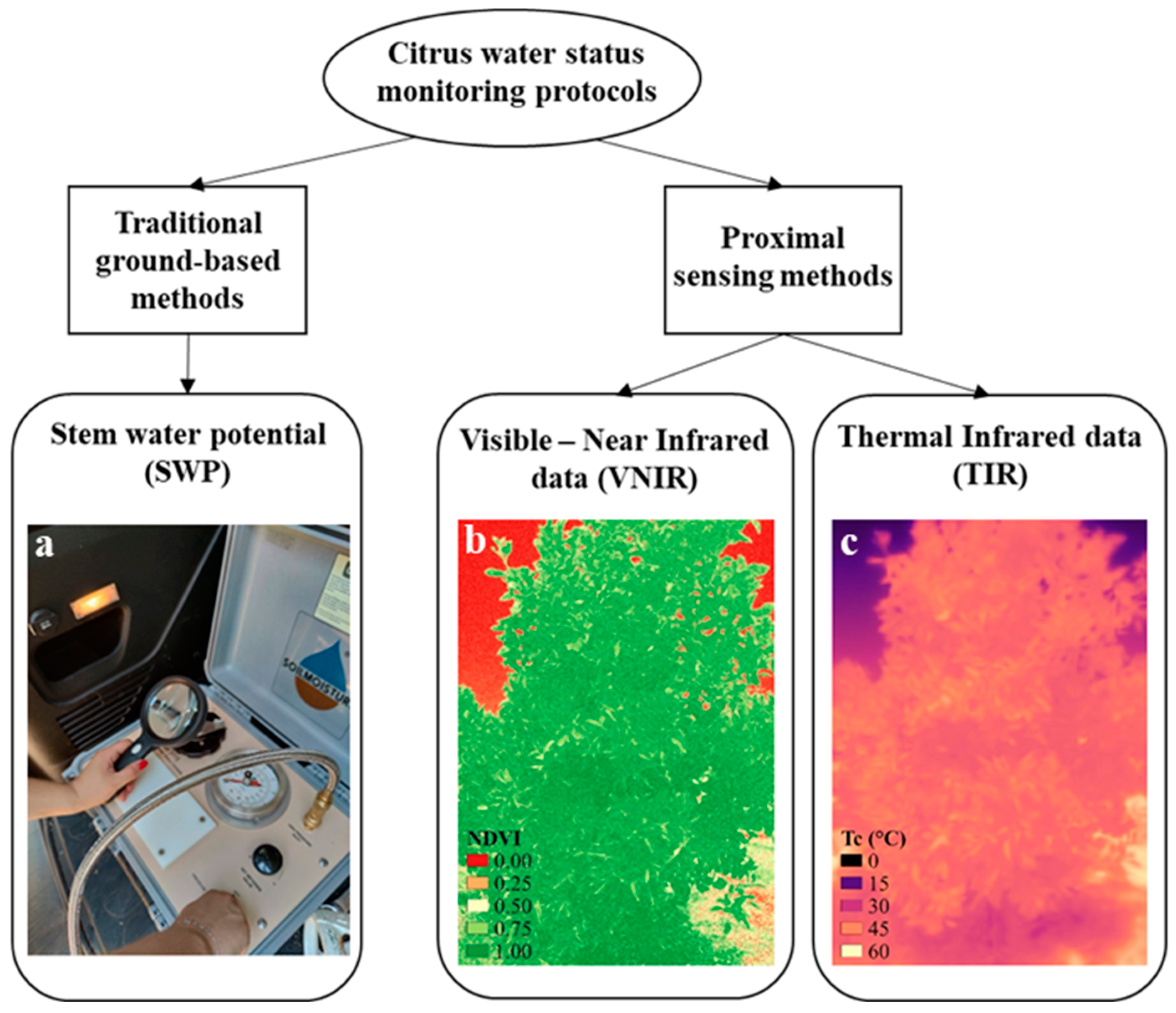
2.2. Methodological Approach

Figure 2 illustrates an overview of the methodological approach proposed in this study to assess the crop water status of orange orchards shown in Figure 1 and Table 1. The proposed approach combined both the use of the traditional Scholander method, for measuring the SWP, and the adoption of proximal sensing tools, based on VNIR and TIR data, for deriving crop physiological proxies.
The acquisition campaign was conducted during the 2023 irrigation season, with one or two monitoring dates in the months of June, July, August, and September (12 dates in total). For each monitoring date, 12 or four trees per WR were monitored at fields 1–2 (24 in total) and fields 3–4 (overall, eight trees), respectively. In August, datasets were acquired only from fields 1–2. The number of trees selected at the fields of interest was dependent on the specific field management characteristics and tree availability in the field. Note that fields 1–2 were part of an experimental farm; conversely, fields 3–4 were located in commercial farms. Note also that no Tc values were recorded in June at Field 3 due to TIR sensor malfunctions.

2.2.1. Stem Water Potential Measurements

Midday SWP measurements were performed using the method described by [24] with a pressure chamber for each date within the reference monitoring period (model 3115, Soilmoisture Equipment Corp., Santa Barbara, CA, USA). Prior to excision, two leaves per tree (overall, 28 trees) were covered with aluminum foil for a minimum of 30 min. Then, the leaves were excised at the base of the petiole to ensure minimal disruption to the water potential and transferred to the pressure chamber, with the petiole inserted through the chamber seal. Once the leaf was secured in the chamber, compressed nitrogen gas was introduced gradually to increase the pressure inside the chamber. The SWP value was recorded when the first drop of xylem was visible at the cut surface. This pressure was assumed to be equivalent to the tension within the xylem [47].

2.2.2. Multispectral Measurements

For each monitoring date, multispectral images of the tree canopies (a total of 336 multispectral images) were acquired under uniform lighting conditions using a low-cost multispectral camera (Mapir Survey3 RGN, San Diego, CA, USA) (https://www.mapir.camera/pages/survey3-cameras#specs, accessed on 1 April 2023). The main technical specifications of the camera are outlined in Table 2.
The multispectral images were subjected to radiometric calibration. In particular, during each image acquisition, the calibration target was also acquired with the same orientation of the tree canopy. The acquired images were converted into reflectance imagery (TIFF format) using the MAPIR Camera Control software (MCC v. 20230123).
The assessment of the crop water status was inferred through the calculation of the NDVI [40] performed in QGIS (V. 3.16), using Equation (1):
NDVI = (NIR − Red)/(NIR + Red)
in which NIR and Red refer to the near-infrared and red spectral bands, respectively.
For each image, the NDVI values were extracted in QGIS by delineating specific regions of interest (ROIs) that only included the tree canopies under study.

2.2.3. Thermal Measurements

TIR information of the tree canopies (Tc) was captured using a low-cost thermal camera (FLIR One Pro, Teledyne FLIR LLC, Arlington, VA, USA), with a total of 336 images acquired during the monitoring period at the same interval as the SWP and VNIR measurements. The technical details of the used thermal camera are given in Table 3.
To guarantee the robustness of the obtained thermal canopy features, these data were extracted from each thermal image on the basis of the delimitation of specific ROIs that included only leaves exposed to sunlight. This choice was made in order to avoid shadow effects, which affect canopy boundary layer temperature and omit mixed pixels on the leaf edge [42].
The ΔT (Tc − Tair) was determined at field level for each monitoring date using the hourly Tair data measured by the closest weather stations managed by SIAS (N.292 and N.234).
In addition, at fields 1–2, the Tc values were also acquired under both non-water stress (Tcold) and non-transpiration (Thot) conditions in order to determine the crop water stress index (CWSI), as shown in Equation (2):
CWSI = (Tc − Tcold)/(Thot − Tcold)
where Tc represents the temperature of the canopy, Tcold is the temperature of a leaf under non-water stress conditions, and Thot is the temperature of a leaf with the stomata completely closed (non-transpiration conditions).
For this purpose, two leaves, facing the eastern side of the canopy, were selected and sprayed with a solution of water and soap in order to obtain Tcold. Furthermore, two additional leaves with identical exposure were coated with petroleum jelly to obtain Thot, thereby ensuring complete stomatal closure. This data collection procedure established the two requisite reference limits for standardizing the effects of atmospheric conditions on transpiration and Tc [37,48]. The complete description of the procedure used in the field for implementing Equation (2) is given in [49,50].
In brief, the TIR data processing procedure included the following steps: (i) the conversion of raw data to .csv format using FLIR Tools (v. 5.3.15320.1002,Teledyne FLIR LLC, Arlington, VA, USA), (ii) the transformation of .csv files into TIFF format images (using a toolbox created in ArcGIS, v. 10.5; ESRI, Redlands, CA, USA), (iii) the identification and digitization of multiple ROIs on the cold and hot reference leaves, and (iv) the extraction of their temperatures for further data analysis computation.

2.2.4. Statistical Analysis

To analyze the datasets acquired in this study (NDVI, Tc, Tc − Tair, CWSI and SWP), the statistical factors ‘WR’, ‘Field’, and ‘Month’ were considered according to the experimental set-up, and, specifically, two WRs (‘WR’, FI versus DI), four different orange orchards (‘Field’, see characteristics in Table 1 and Figure 1), and four separate monitoring periods over the 2023 irrigation season on a monthly basis (‘Month’, i.e., June, July, August and September).
One-way analyses of variance (ANOVAs) were applied to the entire collected datasets to assess significant differences in the single variables under study as a function of the distinct factors ‘WR’, ‘Field’, and ‘Month’. In addition, the datasets were grouped on a monthly basis (June, July, August, and September) and two-way ANOVAs were performed using WR (FI versus DI) and locations (‘Field’) as factors, along with their interactions (WR × Field).
Tukey’s honestly significant difference (HSD) test was applied to identify the observed differences, with the significance level set to p-value < 0.05. The statistical software employed for the purposes of this analysis was Statistix (Version 9.0).

3. Results

3.1. Agrometeorological Data and Irrigation Volumes at the Study Site

Figure 3 illustrates the daily temporal patterns of the main agrometeorological variables monitored during June–September 2023 at the study area, referring to Lentini (N.292) and Paternò (N.234) SIAS stations. In particular, during the study period, the daily average (and standard deviation, ±) Tair values were 23.61 ± 0.24 °C, 29.30 ± 0.51 °C, 26.71 ± 0.63 °C, and 24.29 ± 0.41 °C in June, July, August, and September, respectively. The cumulative average ET0 and rainfall values over the irrigation season were 642 mm and 53 mm, respectively.
The irrigation levels applied at the field sites are reported in Table 4, together with the irrigation savings (%) obtained by adopting the different DI strategies at the field scale (i.e., RDI and PRD, at fields 1–3 and Field 4, respectively). In particular, the cumulative irrigation amounts were 312, 238, 132, and 115 mm at fields 1–4, respectively, corresponding to water savings ranging from 12 to 57% in comparison to the FI, in accordance with the water deficit levels imposed by the DI criteria.

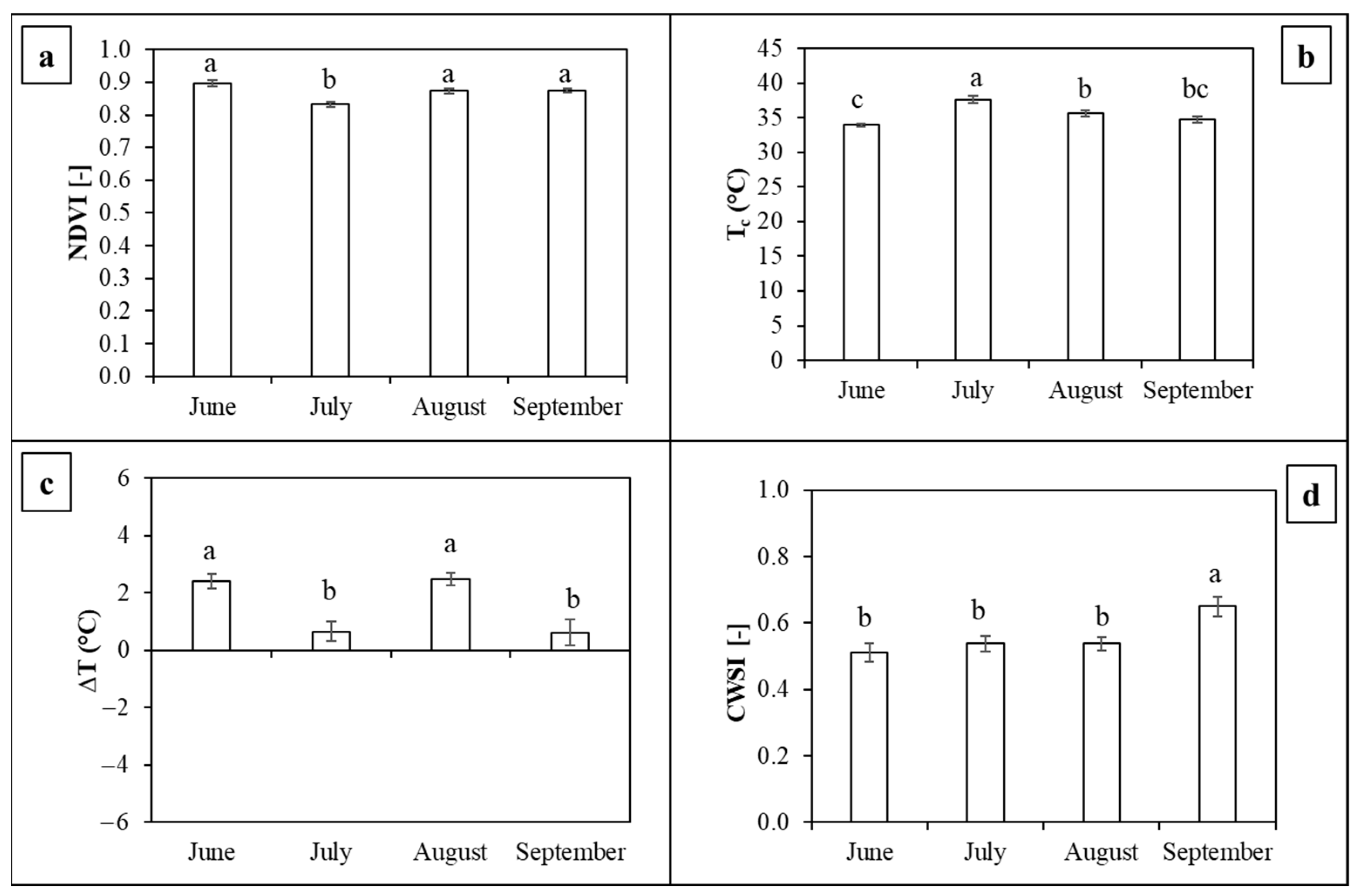
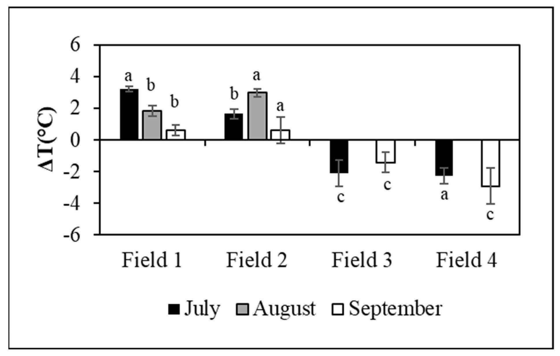
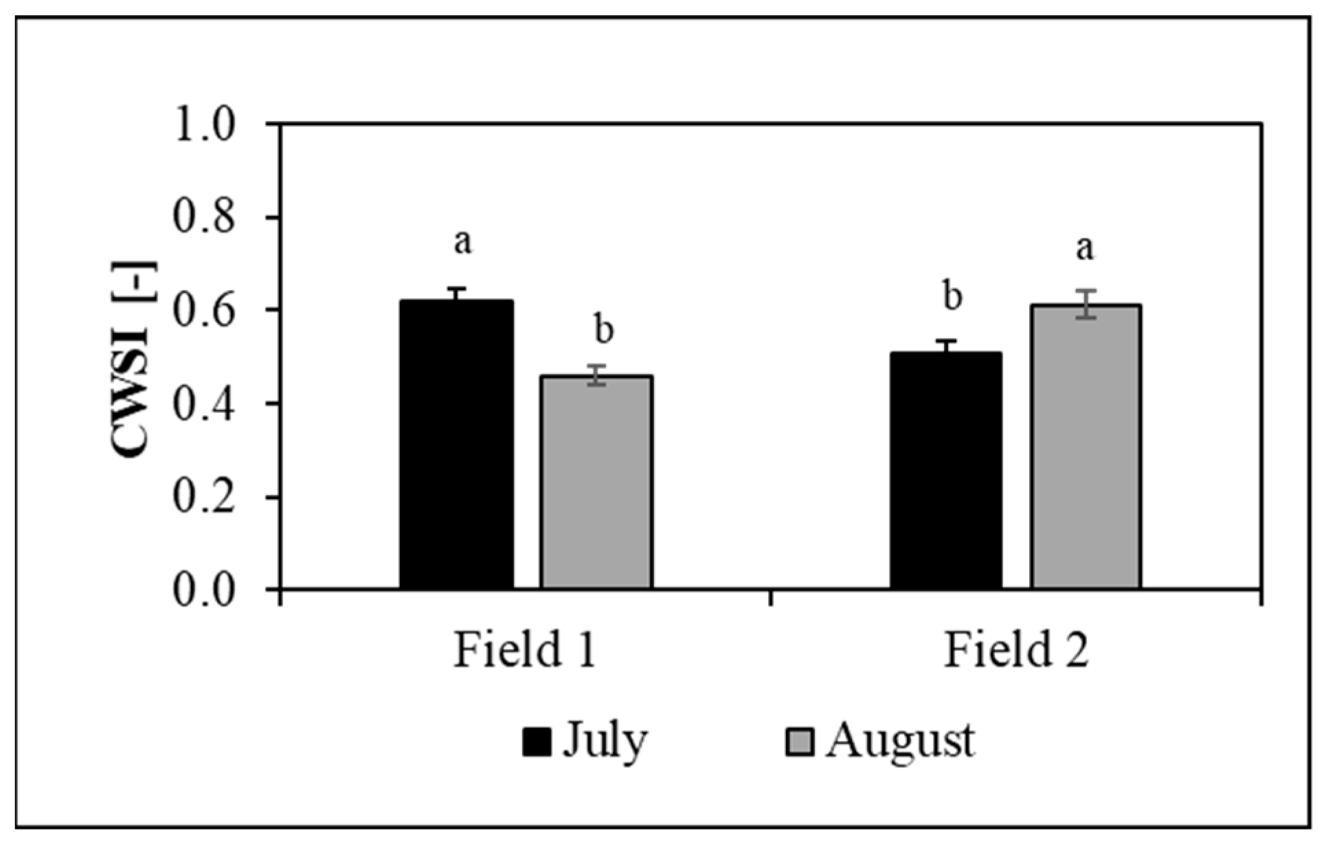
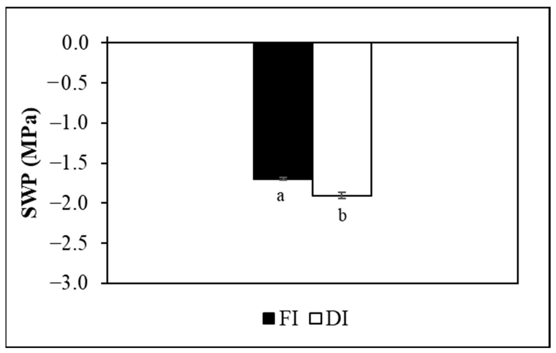
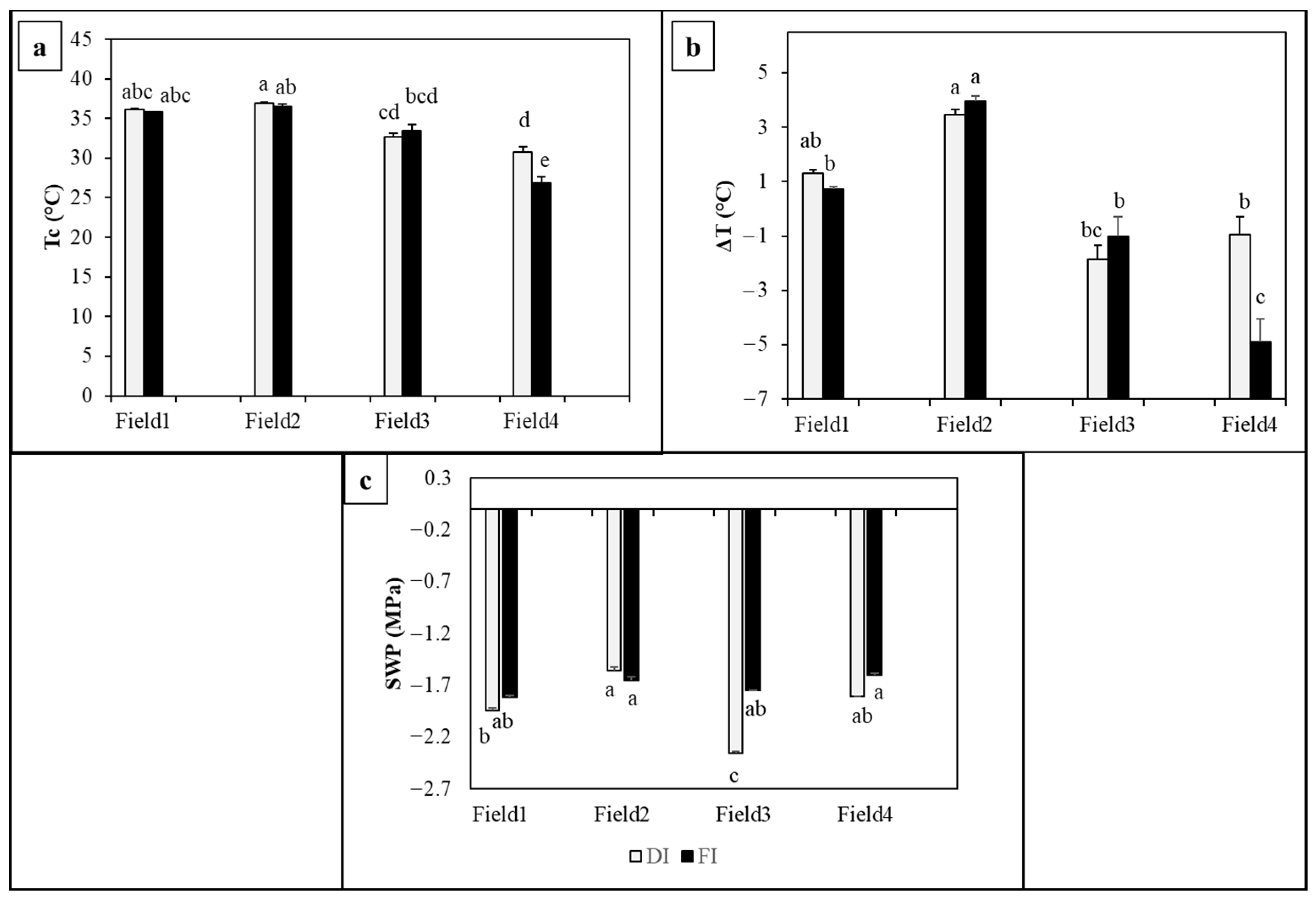
3.2. Effects of Deficit Irrigation Strategies on Citrus Water Status

The results of the one-way ANOVAs applied to the variables NDVI, Tc, Tc − Tair (ΔT), CWSI, and SWP over the overall study period as a function of the single factors ‘WR’, ‘Field’, and ‘Month’ are shown in Table 5, including p-values, degrees of freedom (DF), and F-values (F).
As reported in Table 5, throughout the study period, no differences were observed for the variables of interest (NDVI, Tc, ΔT, CWSI, and SWP) as a function of the applied ‘WRs’. Conversely, differences were found for the same variables, except for the SWP (with an average and standard deviation of −1.63 ± 0.37 MPa), as a function of the ‘Month’ of the year. In particular, lower NDVI values were detected in July (with an average and a standard deviation of 0.83 ± 0.06 compared to 0.88 ± 0.06 in the other months) (Figure 4a). In the same month, the highest Tc values were observed (37.60 ± 3.56 °C), whereas lower values were recorded at the beginning (June) and at the end (September) of the irrigation season (34.34 ± 0.60 °C), with intermediate values in August (35.63± 2.93 °C) (Figure 4b). Higher ΔT (Tc − Tair) was recorded in June and August (2.45 ± 0.06 °C); lower ΔT values were found in July and September (0.76 ± 0.16 °C) (Figure 4c). The CWSI reached its highest value in September (0.65 ± 0.15) (Figure 4d).
As highlighted in Table 5, differences were found also as a function of the ‘Field’ level for all the variables under study, except for CWSI (0.55 ± 0.16). Specifically, lower NDVI values were observed at Field 1 (0.81 ± 0.03) in comparison to the other fields (0.90 ± 0.01) (Figure 5a). Conversely, Field 4 showed the lowest Tc values (32.25 ± 3.30 °C) compared to the other locations (35.87 ± 0.36 °C) (Figure 5b). A higher ΔT (Tc − Tair) was recorded in Field 1 and Field 2 (2.38 ± 0.37 °C); lower ΔT values were found in Field 3 and Field 4 (−0.94 ± 0.34 °C) (Figure 5c). The least negative SWP values were observed at Field 2 (−1.34 ± 0.26 MPa), followed by Field 4 (−1.73 ± 0.16 MPa) and Field 1 (−1.89 ± 0.22 MPa) (Figure 5d). The most negative values were found at Field 3 (−2.04 ± 0.23 MPa) (Figure 5d).
Table 6 reports the main statistical results in terms of p-values, DF, and F-values for the two-way ANOVAs performed on a monthly basis (June, July, August, and September 2023) for the variables NDVI, Tc, Tc − Tair (ΔT), CWSI, and SWP as a function of the ‘WR’ and ‘Field’ factors and their interactions (WR × Field).
As shown in Table 6, differences were found in June for all the variables of interest except for ΔT (Tc − Tair) (2.86 ± 1.36 °C) and CWSI (0.51 ± 0.17) only as a function of the locations (‘Field’). The highest NDVI values were observed in Field 2 (0.94 ± 0.02), followed by Field 4 (0.93 ± 0.01), which behaved similarly to Field 2 and Field 3 (0.91 ± 0.01) (Figure 6a). Conversely, Field 1 exhibited the lowest NDVI values (0.80 ± 0.01) (Figure 6a). The highest Tc value was observed in Field 2 (35.0 ± 0.21 °C), while the lowest values were recorded at fields 1 and 4 (32.9 ± 0.74 °C) (Figure 6b). Note that no Tc values were recorded in June at Field 3 due to a TIR sensor malfunction. For the SWP, the least negative value was observed at Field 2 (−1.21 ± 0.19 MPa). The most negative SWP was recorded in Field 3 (−2.09 ± 0.07 MPa) (Figure 6c). Intermediate values were observed at Field 4 (−1.90 ± 0.06 MPa), followed by Field 1 (−1.72 ± 0.14 MPa) (Figure 6c).
As depicted in Table 6, in July, considerable discrepancies were observed across all variables as a function of the location (‘Field’). The highest NDVI values were observed in Field 3 and Field 4 (0.91 ± 0.02), while the lowest NDVI values were recorded in Field 1 and Field 2 (0.79 ± 0.02) (Figure 6a). For the variable Tc, the lowest values were found in Field 2 and Field 4 (35.9 ±0.78 °C), while the highest values were observed in Field 1 (43.2 ± 0.57). Intermediate Tc values were recorded in Field 3 (37.9 ± 2.31 °C) (Figure 6b). With regard to the ΔT (Tc − Tair), the highest differences were observed in Field 1 (3.12 ± 0.57 °C), whereas the lowest were found in Field 2 (1.29 ± 1.37 °C) (Figure 7). Intermediate ΔT values were noted at Field 3 and Field 4 (−2.18 ± 0.11 °C) (Figure 7). The highest CWSI values were observed in Field 1 (0.64 ± 0.07), while the lowest values were observed in Field 2 (0.48 ± 0.14) (Figure 8). For SWP, the lowest value was observed in fields 1 and 3 (−2.05 ± 0.11 MPa), intermediate values were recorded at Field 4 (−1.6 ± 0.09 MPa), and the highest value was recorded at Field 2 (−1.23 ± 0.23 MPa) (Figure 6c).
As highlighted in Table 6, in August, all the variables under study showed a site-dependent pattern in fields 1–2. Higher NDVI values were observed in Field 2 (0.92 ± 0.04), whereas lower values were recorded in Field 1 (0.82 ± 0.02) (Figure 6a). With regard to Tc, lower values were observed in Field 1 (34.03 ± 3.14 °C), whereas higher Tc values were found in Field 2 (37.2 ± 1.56 °C) (Figure 6b). For ΔT, the highest and lowest discrepancies were obtained in Field 2 (2.99 ± 1.22 °C) and Field 1 (1.78± 1.38 °C), respectively (Figure 7). In terms of CWSI, higher and lower values were recorded in Field 2 (0.61 ± 0.14) and Field 1 (0.46 ± 0.09), respectively (Figure 8). This trend was also confirmed for SWP, resulting in more negative and less negative values in Field 1 (−1.86 ± 0.20 MPa) and Field 2 (−1.32 ± 0.20 MPa), respectively (Figure 6c).
During the final part of the irrigation season, in September, differences were found for all the variables of interest as a function of the location (‘Field’), except for CWSI (Table 6). For NDVI, the highest and lowest values were found in fields 3–4 (0.91 ± 0.01) and fields 1–2 (0.86 ± 0.02), respectively (Figure 6a). For Tc, the lowest and highest values were found in Field 4 (28.8 ± 3.2 °C) and fields 1–2 (36.3 ± 0.5 °C), whereas intermediate conditions were detected in Field 3 (33.1 ± 1.7 °C) (Figure 6b). For ΔT, the highest and lowest differences were observed in Field 2 (3.7 ± 1.34 °C) and fields 3–4 (−2.2 ± °C), while intermediate values were recorded in Field 1 (0.99 ± 0.67 °C) (Figure 7). Less negative SWP values were found in Field 2 (−1.60 ± 0.11 MPa) and Field 4 (−1.70 ± 0.11 MPa). The latter showed similar SWP values to Field 1 (−1.88 ± 0.11 MPa), which resulted in more negative SWP values similar to Field 3 (−2.05 ± 0.33MPa) (Figure 6c).
In September, the SWP was also affected by the ‘WR’ factor, resulting in more negative values under the DI (−1.91 ± 0.38 MPa) compared to FI (−1.70 ± 0.17 MPa) (Figure 9). During the same month, interactions between ‘WR’ and ‘Field’ were obtained for Tc, ΔT, and SWP according to the results reported in Figure 10a–c.

4. Discussion

Nowadays, the increased technological development of sensing devices has opened new prospects for providing sensor-based indicators of crop water status [51,52]. In general, the use of VNIR and TIR information has provided useful proxies for appraising the crop physiological conditions in situ compared to plant-based measurements [53]. Although TIR sensing has several potential advantages for crop water stress detection over VNIR information, there are important challenges that need to be solved for precision agriculture applications [54]. Notably, both VIs and Tc-based measurements are susceptible to uncertainties due to the variability in agrometeorological variables, such as cloud cover and/or wind speed, which may alter the spectral response of the canopy [32,55,56,57]. In this sense, it is recommended to conduct the proximal sensing data acquisition phase under homogenous agrometeorological conditions [58]. Moreover, some TIR indices, including CWSI, need to be calibrated in situ by collecting site-specific information (i.e., Tcold and Thot) to be carefully computed [50]. The implementation of these procedures may limit the use of the CWSI for operational purposes, under any agrometeorological condition, suggesting the adoption of empirical baselines [59,60].
In this study, the potential of using commercial low-cost proximal sensors based on VNIR and TIR data was explored as an alternative approach to overcome the limitations of traditional plant-based methods (such as SWP-based methods) for characterizing the water status of citrus groves irrigated under different WRs (FI and DI) and under multiple cultivar/rootstock combinations and locations (Figure 1 and Table 1). The innovative methodological approach proposed in this study offers several practical advantages, including accessibility, economic viability, and reduced resource requirements for device installation and/or maintenance compared to the employment of plant-based sensors (e.g., sap flow probes, dendrometers) [61].
Furthermore, the findings of this study are consistent with the observations provided by other studies [62,63,64,65], which recognize the spatial and temporal dependency of VIs and TIR-based indicators on crop water status characteristics. In particular, the results of this study contribute to highlighting the role of environmental and crop management conditions in influencing citrus water status responses in terms of TIR and VNIR data throughout the irrigation season (Table 5). Specifically, the results of the one-way ANOVAs at the ‘Month’ level revealed that NDVI exhibited lower values in July than in other months (Figure 4a), indicating a reduction in photosynthetic activity due to the thermal stress experienced in that period [62]. This decline in NDVI was consistent with higher Tc values observed in the same month, coinciding with the peak in atmospheric demand and solar radiation (Figure 4b). These results corroborate earlier findings that lower NDVI values are typically observed during periods of maximum heat stress [63,65]. Conversely, NDVI values were relatively higher in June and September, suggesting less stressful environmental conditions for the orange trees during these months (Figure 4a,b). However, the peak of ΔT observed in the months of June and August (Figure 4c) suggests a reduced stomatal activity compared to July and September [66]. Specifically, in the month of September, even when Tair conditions improved, the maximum CWSI values were reached as a cumulative effect of the applied water deficit (Figure 4d) [67,68].
The one-way ANOVAs for the ’Field’ factor revealed significant discrepancies in most of the analyzed variables (Table 5). For example, the lowest NDVI values were observed in Field 1 (Figure 5a), a phenomenon which may be attributed to site-specific factors including soil characteristics, tree age (i.e., more than 20 years old), and/or microclimatic conditions (such as exposure to solar radiation, elevation above sea level, a.s.l.), and/or different tree spacing at the field sites (Table 1). Microclimatic variations among fields can amplify NDVI differences, particularly under water stress conditions [63]. Additionally, older orange trees may exhibit increased vulnerability to water stress [69]. In this study, significant variations were also evident in Tc at the ‘Field’ level (Figure 5b). For instance, Field 4 recorded the lowest Tc values, suggesting a more favorable microclimatic condition (Figure 5b). Similarly, ΔT exhibited a systematic pattern between fields 1–2 and fields 3–4, according to the local environmental conditions (Figure 5c). Notably, fields 1–2 were located on the same farm (Lentini), whereas fields 3–4 were situated in Motta S. Anastasia and Misterbianco, respectively (Figure 1 and Table 1).
The results of the two-way ANOVAs corroborate that, on a monthly basis, most of the analyzed variables were mainly affected by site-specific conditions (‘Field’) (Figure 6, Figure 7 and Figure 8). Interestingly, at the end of the irrigation season (in September), SWP showed a more negative trend under DI conditions (Figure 9). These findings align with the applied water deficits, resulting in SWP values lower than those of the well-watered citrus tree threshold (i.e., −1.32 MPa) [70]. Additionally, at the same time step, discrepancies were observed as a function of the interaction between ‘Field’ and ‘WR’, in terms of Tc, ΔT, and SWP, highlighting the cumulative effects of WR applications at the end of the irrigation season (Figure 10) [68].

5. Conclusions

This study emphasizes the utility of a methodological approach based on low-cost VNIR and TIR proximal sensors for assessing the significance of different water status indicators in multiple citrus groves (including different cultivars/rootstocks and locations) subjected to different WRs (FI versus DI). Herein, significant differences were found for some of the analyzed biophysical variables among the field sites (NDVI, Tc, ΔT, and SWP) and across time periods (NDVI, Tc, ΔT, and CWSI), demonstrating that environmental and management factors exert a decisive influence on complex crop physiological responses. For instance, NDVI declined by 6% in July compared to other months, coinciding with high Tc levels recorded in the same period. A cumulative effect of water deficit was discerned at the end of the irrigation season (in September), characterized by CWSI values reaching 0.65. During the same period, more negative SWP values were recorded under DI (−1.91 ± 0.38 MPa) compared to FI (−1.70 ± 0.17 MPa) conditions. Additionally, interactions between WR and citrus groves were also observed for SWP, Tc, and ΔT. The behavior of the analyzed variables was linked to the microclimatic conditions, resulting in lower ΔT values under more favorable environments (fields 3–4). Conversely, an independent trend was observed for SWP, NDV, and Tc due to the site-specific characteristics of the fields, highlighting the importance of conducting smart and efficient measurements at the plant level.
In conclusion, the study provides an innovative methodological framework for precision irrigation applications which addresses the limitations of conventional methods in terms of operational efforts and high costs associated with determining crop water status indicators (e.g., pressure chambers). Additionally, the adoption of low-cost TIR and VNIR sensors may contribute to a more comprehensive understanding of the complex spatial and temporal variability of citrus water status proxies.

Author Contributions

Conceptualization: S.C., G.L.-M. and D.V.; data curation: S.T., G.L.-M., A.C., G.M. and S.G.; formal analysis: S.T.; funding acquisition: S.C., A.C., A.G. and S.B.; investigation: S.T., S.C., G.L.-M., A.C., G.M., A.G., S.G., S.B., D.V. and G.L.C.; methodology: S.T., S.C., G.L.-M., A.C., S.G. and D.V.; supervision: S.C. and D.V.; visualization: S.T., G.L.-M. and D.V.; writing—original draft: S.T. and D.V.; writing—review and editing: S.C., G.L.-M., G.M., A.C., G.L.C. and D.V. All authors have read and agreed to the published version of the manuscript.

Funding

This work was carried out within the framework of the project Agritech National Research Center funded by the European Union Next-GenerationEU (PIANO NAZIONALE DI RIPRESA E RESILIENZA (PNRR)—MISSIONE 4 COMPONENTE 2, INVESTIMENTO 1.4—D.D. 1032 17 June 2022, CN00000022), the project Innovazioni nel comparto agrumicolo e risparmio idrico attraverso tecniche di agricoltura di precisione—IRRIAP (Mis. 16.1 del PSR-Sicilia 2014/2022), and the research project of National relevance (PRIN 2022) entitled Smart Technologies and Remote Sensing methods to support the sustainable Agriculture WAter Management of Mediterranean woody Crops—SWAM4Crops (2022SC3CNE, CUP E53D23010950001).

Data Availability Statement

The original contributions presented in the study are included in the article; further inquiries can be directed to the corresponding author.

Acknowledgments

The authors wish to thank the researchers and the personnel of Consiglio per la ricerca in agricoltura e l’analisi dell’economia agraria, Centro di Ricerca Olivicoltura, Frutticoltura e Agrumicoltura (CREA-OFA) of Acireale (CT) for their hospitality at the Fields 1–2, and the commercial farms Bonomo and Crispi (Fields 3–4). In addition, the authors acknowledge Filippo Ferlito, and Marco Caruso (CREA-OFA) for selecting the rootstocks used at Field 2.

Conflicts of Interest

The authors declare no conflicts of interest.

References

  1. Morante-Carballo, F.; Montalván-Burbano, N.; Quiñonez-Barzola, X.; Jaya-Montalvo, M.; Carrión-Mero, P. What Do We Know about Water Scarcity in Semi-Arid Zones? A Global Analysis and Research Trends. Water 2022, 14, 2685. [Google Scholar] [CrossRef]
  2. Vargas, J.; Paneque, P. Challenges for the Integration of Water Resource and Drought-Risk Management in Spain. Sustainability 2019, 11, 308. [Google Scholar] [CrossRef]
  3. Vicente-Serrano, S.M.; Miralles, D.G.; McDowell, N.; Brodribb, T.; Domínguez-Castro, F.; Leung, R.; Koppa, A. The Uncertain Role of Rising Atmospheric CO2 on Global Plant Transpiration. Earth-Sci. Rev. 2022, 230, 104055. [Google Scholar] [CrossRef]
  4. Arnone, E.; Pumo, D.; Viola, F.; Noto, L.V.; La Loggia, G. Rainfall statistics changes in Sicily. Hydrol. Earth Syst. Sci. 2013, 17, 2449–2458. [Google Scholar] [CrossRef]
  5. Viola, F.; Liuzzo, L.; Noto, L.V.; Conti, F.; La Loggia, G. Spatial Distribution of Temperature Trends in Sicily. Int. J. Climatol. 2014, 34, 1–17. [Google Scholar] [CrossRef]
  6. Consoli, S.; Stagno, F.; Roccuzzo, G.; Cirelli, G.L.; Intrigliolo, F. Sustainable Management of Limited Water Resources in a Young Orange Orchard. Agric. Water Manag. 2014, 132, 71–80. [Google Scholar] [CrossRef]
  7. Consoli, S.; Stagno, F.; Vanella, D.; Boaga, J.; Cassiani, G.; Roccuzzo, G. Partial Root-Zone Drying Irrigation in Orange Orchards: Effects on Water Use and Crop Production Characteristics. Eur. J. Agron. 2017, 82, 190–202. [Google Scholar] [CrossRef]
  8. Ciriminna, R.; Angellotti, G.; Luque, R.; Pagliaro, M. The Citrus Economy in Sicily in the Early Bioeconomy Era: A Case Study for Bioeconomy practitioners. Biofuels Bioprod. Bioref. 2024, 18, 356–364. [Google Scholar] [CrossRef]
  9. Fares, A.; Bayabil, H.K.; Zekri, M.; Mattos, D., Jr.; Awal, R. Potential Climate Change Impacts on Citrus Water Requirement Major Producing Areas in the World. J. Water Clim. Chang. 2017, 8, 576–592. [Google Scholar] [CrossRef]
  10. Sthowski, P.; Jagosz, B.; Rolbiecki, S.; Rolbiecki, R. Predictive Capacity of Rainfall Data to Estimate the Water Needs of Fruit Plants in Water Deficit Areas. Atmosphere 2021, 12, 550. [Google Scholar] [CrossRef]
  11. Berríos, P.; Temnani, A.; Zapata-García, S.; Sánchez-Navarro, V.; Zornoza, R.; Pérez-Pastor, A. Effect of Deficit Irrigation and Mulching on the Agronomic and Physiological Response of Mandarin Trees as Strategies to Cope with Water Scarcity in a Semi-Arid Climate. Sci. Hortic. 2024, 324, 112572. [Google Scholar] [CrossRef]
  12. Vanella, D.; Ferlito, F.; Torrisi, B.; Giuffrida, A.; Pappalardo, S.; Saitta, D.; Longo-Minnolo, G.; Consoli, S. Long-Term Monitoring of Deficit Irrigation Regimes on Citrus Orchards in Sicily. J. Agric. Eng. 2021, 52, 1–9. [Google Scholar] [CrossRef]
  13. Saitta, D.; Consoli, S.; Ferlito, F.; Torrisi, B.; Allegra, M.; Longo-Minnolo, G.; Vanella, D. Adaptation of Citrus Orchards to Deficit Irrigation Strategies. Agric. Water Manag. 2021, 247, 106734. [Google Scholar] [CrossRef]
  14. Capra, A.; Consoli, S.; Russo, A.; Scicolone, B. Integrated Agro-Economic Approach to Deficit Irrigation on Lettuce Crops in Sicily (Italy). J. Irrig. Drain. Eng. 2008, 134, 437–445. [Google Scholar] [CrossRef]
  15. Gasque, M.; Martí, P.; Granero, B.; González-Altozano, P. Effects of Long-Term Summer Deficit Irrigation on ‘Navelina’ Citrus Trees. Agric. Water Manag. 2016, 169, 140–147. [Google Scholar] [CrossRef]
  16. González-Dugo, V.; Ruz, C.; Testi, L.; Orgaz, F.; Fereres, E. The Impact of Deficit Irrigation on Transpiration and Yield of Mandarin and Late Oranges. Irrig. Sci. 2018, 36, 227–239. [Google Scholar] [CrossRef]
  17. Zhang, J.H.; Schurr, U.; Davies, W.J. Control of Stomatal Behavior by Abscisic-Acid Which Apparently Originates in the Roots. J. Exp. Bot. 1987, 38, 1174–1181. [Google Scholar] [CrossRef]
  18. Davies, W.J.; Hartung, W. The Nexus between Root Signals and Stomatal Control: New Insights from Partial Rootzone Drying. Plant Cell Environ. 2004, 27, 69–87. [Google Scholar]
  19. Kang, S.; Zhang, J. Controlled Alternate Partial Root-Zone Irrigation: Its Physiological Consequences and Impact on Water Use Efficiency. J. Exp. Bot. 2004, 55, 2437–2446. [Google Scholar] [CrossRef]
  20. Sepaskhah, A.; Ahmadi, S.H. A Review on Partial Root-Zone Drying Irrigation. Int. J. Plant Prod. 2010, 4, 1735–6814. [Google Scholar]
  21. Pérez-Pérez, J.G.; Navarro, J.M.; Robles, J.M.; Dodd, I.C. Prolonged Drying Cycles Stimulate ABA accumulation in Citrus Macrophylla Seedlings Exposed to Partial Rootzone Drying. Agric. Water Manag. 2018, 210, 271–278. [Google Scholar] [CrossRef]
  22. Rallo, G.; Paço, T.A.; Paredes, P.; Puig-Sirera, A.; Massai, R.; Provenzano, G.; Pereira, L.S. Updated Single and Dual Crop Coefficients for Tree and Vine Fruit Crops. Agric. Water Manag. 2021, 250, 106645. [Google Scholar] [CrossRef]
  23. Fernández, J.E.; Padilla-Díaz, C.M.; Martínez, G.; Fernández, A.; Pérez-Ruiz, M. Advanced Irrigation Scheduling Techniques: Using Sensors and Remote Sensing for Improving Water Use in Agriculture. Agric. Water Manag. 2020, 240, 106270. [Google Scholar] [CrossRef]
  24. Scholander, P.F.; Hammel, H.T.; Bradstreet, E.D.; Hemmingsen, E.A. Sap Pressure in Vascular Plants. Science 1965, 148, 339–346. [Google Scholar] [CrossRef]
  25. Turner, M.G.; Baker, W.L.; Peterson, C.J.; Peet, R.K. Factors Influencing Succession: Lessons from Large, Infrequent Natural Disturbances. Ecosystems 1998, 1, 511–523. [Google Scholar] [CrossRef]
  26. Cohen, Y.; Alchanatis, V.; Saranga, Y.; Rosenberg, O.; Sela, E.; Bosak, A.J.P.A. Mapping Water Status Based on Aerial Thermal Imagery: Comparison of Methodologies for Upscaling from a Single Leaf to Commercial Fields. Precis. Agric. 2017, 18, 801–822. [Google Scholar] [CrossRef]
  27. Han, M.; Zhang, H.; DeJonge, K.C.; Comas, L.H.; Gleason, S. Comparison of Three Crop Water Stress Index Models with Sap Flow Measurements in Maize. Agric. Water Manag. 2018, 203, 366–375. [Google Scholar] [CrossRef]
  28. Caruso, G.; Palai, G.; Gucci, R.; Priori, S. Remote and Proximal Sensing Techniques for Site-Specific Irrigation Management in the Olive Orchard. Appl. Sci. 2022, 12, 1309. [Google Scholar] [CrossRef]
  29. Darra, N.; Psomiadis, E.; Kasimati, A.; Anastasiou, A.; Anastasiou, E.; Fountas, S. Remote and Proximal Sensing-Derived Spectral Indices and Biophysical Variables for Spatial Variation Determination in Vineyards. Agronomy 2021, 11, 741. [Google Scholar] [CrossRef]
  30. Ben-Gal, A.; Agam, N.; Alchanatis, V.; Cohen, Y.; Yermiyahu, U.; Zipori, I.; Presnov, E.; Sprintsin, M.; Dag, A. Evaluating Water Stress in Irrigated Olives: Correlation of Soil Water Status, Tree Water Status, and Thermal Imagery. Irrig. Sci. 2009, 27, 367–376. [Google Scholar] [CrossRef]
  31. Egea, G.; Padilla-Díaz, C.M.; Martínez, J.; Fernández, J.E.; Pérez-Ruiz, M. Use of Aerial Thermal Imaging to Assess Water Status Variability in Hedgerow Olive Orchards. Agric. Water Manag. 2016, 187, 210–219. [Google Scholar] [CrossRef]
  32. García-Tejero, I.F.; Ortega-Arévalo, C.J.; Iglesias-Contreras, M.; Moreno, J.M.; Souza, L.; Tavira, S.C.; Durán-Zuazo, V.H. Assessing the Crop-Water Status in Almond (Prunus dulcis Mill.) Trees via Thermal Imaging Camera Connected to Smartphone. Sensors 2018, 18, 1050. [Google Scholar] [CrossRef] [PubMed]
  33. Blanco, V.; Willsea, N.; Campbell, T.; Howe, O.; Kalcsits, L. Combining Thermal Imaging and Soil Water Content Sensors to Assess Tree Water Status in Pear Trees. Front. Plant Sci. 2023, 14, 1197437. [Google Scholar] [CrossRef]
  34. Ballester, C.; Jiménez-Bello, M.A.; Castel, J.R.; Intrigliolo, D.S. Usefulness of Thermography for Plant Water Stress Detection in Citrus and Persimmon Trees. Agric. For. Meteorol. 2013, 168, 120–129. [Google Scholar] [CrossRef]
  35. Mangus, D.L.; Sharda, A.; Zhang, N. Development and Evaluation of Thermal Infrared Imaging System for High Spatial and Temporal Resolution Crop Water Stress Monitoring of Corn within a Greenhouse. Comput. Electron. Agric. 2016, 121, 149–159. [Google Scholar] [CrossRef]
  36. Möller, M.; Alchanatis, V.; Cohen, Y.; Meron, M.; Tsipris, J.; Naor, A.; Ostrovsky, V.; Sprintsin, M.; Cohen, S. Use of Thermal and Visible Imagery for Estimating Crop Water Status of Irrigated Grapevine. J. Exp. Bot. 2007, 58, 827–838. [Google Scholar] [CrossRef]
  37. Idso, S.B.; Jackson, R.D.; Reginato, R.J. Normalizing the Stress-Degree-Day Parameter for Environmental Variability. Agric. Meteorol. 1981, 24, 45–55. [Google Scholar] [CrossRef]
  38. González-Dugo, V.; Zarco-Tejada, P.J.; Fereres, E. Applicability and Limitations of Using the Crop Water Stress Index as an Indicator of Water Deficits in Citrus Orchards. Agric. For. Meteorol. 2014, 198, 94–104. [Google Scholar] [CrossRef]
  39. Jamshidi, S.; Zand-Parsa, S.; Niyogi, D. Assessing Crop Water Stress Index of Citrus Using In-Situ Measurements, Landsat, and Sentinel-2 Data. Int. J. Remote Sens. 2021, 42, 1893–1916. [Google Scholar] [CrossRef]
  40. Rouse, J.W.; Haas, R.H.; Schell, J.A.; Deering, D.W. Monitoring Vegetation Systems in the Great Plains with ERTS. NASA Spec. Publ. 1974, 351, 309. [Google Scholar]
  41. El-Hendawy, S.E.; Al-Suhaibani, N.; Alotaibi, M.; Hassan, W.; Elsayed, S.; Tahir, M.U.; Ahmed Ibrahim Mohamed, A.I.; Schmidhalter, U. Estimating growth and photosynthetic properties of wheat grown in simulated saline field conditions using hyperspectral reflectance sensing and multivariate analysis. Sci. Rep. 2019, 9, 1647. [Google Scholar] [CrossRef] [PubMed]
  42. Fernandes de Oliveira, A.; Mameli, M.G.; Lo Cascio, M.; Sirca, C.; Satta, D. An index for user-friendly proximal detection of water requirements to optimized irrigation management in vineyards. Agronomy 2021, 11, 323. [Google Scholar] [CrossRef]
  43. Pou, A.; Diago, M.P.; Medrano, H.; Baluja, J.; Tardaguila, J. Validation of thermal indices for water status identification in grapevine. Agric. Water Manag. 2014, 134, 60–72. [Google Scholar] [CrossRef]
  44. Abbatantuono, F.; Lopriore, G.; Tallou, A.; Brillante, L.; Ali, S.A.; Camposeo, S.; Vivaldi, G.A. Recent progress on grapevine water status assessment through remote and proximal sensing: A review. Sci. Hortic. 2024, 338, 113658. [Google Scholar] [CrossRef]
  45. Panagos, P.; Van Liedekerke, M.; Borrelli, P.; Köninger, J.; Ballabio, C.; Orgiazzi, A.; Lugato, E.; Liakos, L.; Hervas, J.; Jones, A.; et al. European Soil Data Centre 2.0: Soil data and knowledge in support of the EU policies. Eur. J. Soil Sci. 2022, 73, e13315. [Google Scholar] [CrossRef]
  46. Allen, R.G.; Pereira, L.S.; Raes, D.; Smith, M. Crop Evapotranspiration—Guidelines for Computing Crop Water Requirements. FAO Irrig. Drain. Pap. 1998, 56, 147–151. [Google Scholar]
  47. Flo, V.; Martínez-Vilalta, J.; Mencuccini, M.; Granda, V.; Anderegg, W.R.; Poyatos, R. Climate and functional traits jointly mediate tree water-use strategies. New Phytol. 2021, 231, 617–630. [Google Scholar] [CrossRef] [PubMed]
  48. Jakson, R.D.; Idso, S.B.; Reginato, R.J.; Pinter, P.J. Canopy Temperature as a Crop Water Stress Indicator. Water Resour. Res. 1981, 17, 1133–1138. [Google Scholar] [CrossRef]
  49. Ramírez-Cuesta, J.M.; Ortuno, M.F.; Gonzalez-Dugo, V.; Zarco-Tejada, P.J.; Parra, M.; Rubio-Asensio, J.S.; Intrigliolo, D.S. Assessment of peach trees water status and leaf gas exchange using on-the-ground versus airborne-based thermal imagery. Agric. Water Manag. 2022, 267, 107628. [Google Scholar] [CrossRef]
  50. Pappalardo, S.; Consoli, S.; Longo-Minnolo, G.; Vanella, D.; Longo, D.; Guarrera, S.; Ramírez-Cuesta, J.M. Performance Evaluation of a Low-Cost Thermal Camera for Citrus Water Status Estimation. Agric. Water Manag. 2023, 288, 108489. [Google Scholar] [CrossRef]
  51. Kitić, G.; Tagarakis, A.; Cselyuszka, N.; Panić, M.; Birgermajer, S.; Sakulski, D.; Matović, J. A New Low-Cost Portable Multispectral Optical Device for Precise Plant Status Assessment. Comput. Electron. Agric. 2019, 162, 300–308. [Google Scholar] [CrossRef]
  52. Rajak, P.; Ganguly, A.; Adhikary, S.; Bhattacharya, S. Internet of Things and smart sensors in agriculture: Scopes and challenges. J. Agric. Food Res. 2023, 14, 100776. [Google Scholar] [CrossRef]
  53. Xie, J.; Chen, Y.; Yu, Z.; Wang, J.; Liang, G.; Gao, P.; Li, J. Estimating Stomatal Conductance of Citrus under Water Stress Based on Multispectral Imagery and Machine Learning Methods. Front. Plant Sci. 2023, 14, 1054587. [Google Scholar] [CrossRef]
  54. Gerhards, M.; Schlerf, M.; Mallick, K.; Udelhoven, T. Challenges and future perspectives of multi-/Hyperspectral thermal infrared remote sensing for crop water-stress detection: A review. Remote Sens. 2019, 11, 1240. [Google Scholar] [CrossRef]
  55. Jones, H.G. Irrigation scheduling: Advantages and pitfalls of plant-based methods. J. Exp. Bot. 2004, 55, 2427–2436. [Google Scholar] [CrossRef]
  56. García-Tejero, I.F.; Hernández, A.; Padilla-Díaz, C.M.; Diaz-Espejo, A.; Fernandez, J.E. Assessing plant water status in a hedgerow olive orchard from thermography at plant level. Agric. Water Manag. 2017, 188, 50–60. [Google Scholar] [CrossRef]
  57. Petrie, P.R.; Wang, Y.; Liu, S.; Lam, S.; Whitty, M.A.; Skewes, M.A. The accuracy and Utility of a Low-Cost Thermal Camera and Smartphone-Based System to Assess Grapevine Water Status. Biosyst. Eng. 2019, 179, 126–139. [Google Scholar] [CrossRef]
  58. Ramírez-Cuesta, J.M.; Consoli, S.; Longo, D.; Longo-Minnolo, G.; Intrigliolo, D.S.; Vanella, D. Influence of Short-Term Temperature Dynamics on Tree Orchards Energy Balance Fluxes. Precis. Agric. 2022, 23, 1394–1412. [Google Scholar] [CrossRef]
  59. Katimbo, A.; Rudnick, D.R.; DeJonge, K.C.; Lo, T.H.; Qiao, X.; Franz, T.E.; Duan, J. Crop Water Stress Index Computation Approaches and Their Sensitivity to Soil Water Dynamics. Agric. Water Manag. 2022, 266, 107575. [Google Scholar] [CrossRef]
  60. Irmak, S.; Haman, D.Z.; Bastug, R. Determination of Crop Water Stress Index for Irrigation Timing and Yield Estimation of Corn. Agron. J. 2000, 92, 1221–1227. [Google Scholar] [CrossRef]
  61. Camino, C.; Zarco-Tejada, P.J.; González-Dugo, V. Effects of Heterogeneity within Tree Crowns on Airborne-Quantified SIF and the CWSI as Indicators of Water Stress in the Context of Precision Agriculture. Remote Sens. 2018, 10, 604. [Google Scholar] [CrossRef]
  62. Conesa, M.R.; Conejero, W.; Vera, J.; Mira-García, A.B.; Ruiz-Sánchez, M.C. Impact of a DANA Event on the Thermal Response of Nectarine Trees. Plants 2023, 12, 907. [Google Scholar] [CrossRef]
  63. González-Dugo, V.; Zarco-Tejada, P.J.; Fereres, E. Assessing the Impact of Measurement Errors in the Calculation of CWSI for Characterizing the Water Status of Several Crop Species. Irrig. Sci. 2022, 42, 10–19. [Google Scholar] [CrossRef]
  64. Longo-Minnolo, G.; Vanella, D.; Consoli, S.; Intrigliolo, D.S.; Ramírez-Cuesta, J.M. Integrating Forecast Meteorological Data into the ArcDualKc Model for Estimating Spatially Distributed Evapotranspiration Rates of a Citrus Orchard. Agric. Water Manag. 2020, 231, 105967. [Google Scholar] [CrossRef]
  65. Velazquez-Chavez, L.J.; Daccache, A.; Mohamed, A.Z.; Centritto, M. Plant-based and remote sensing for water status monitoring of orchard crops: Systematic review and meta-analysis. Agric. Water Manag. 2024, 303, 109051. [Google Scholar] [CrossRef]
  66. Corak, N.K.; Otkin, J.A.; Ford, T.W.; Lowman, L.E.L. Unraveling Phenological and Stomatal Responses to Flash Drought and Implications for Water and Carbon Budgets. Hydrol. Earth Syst. Sci. 2024, 28, 1827–1850. [Google Scholar] [CrossRef]
  67. Bellvert, J.; Marsal, J.; Girona, J.; Gonzalez-Dugo, V.; Fereres, E.; Ustin, S.L.; Zarco-Tejada, P.J. Airborne thermal imagery to detect the seasonal evolution of crop water status in peach, nectarine and Saturn peach orchards. Remote Sens. 2016, 8, 39. [Google Scholar] [CrossRef]
  68. Puglisi, I.; Nicolosi, E.; Vanella, D.; Lo Piero, A.R.; Stagno, F.; Saitta, D.; Roccuzzo, G.; Consoli, S.; Baglieri, A. Physiological and biochemical responses of orange trees to different deficit irrigation regimes. Plants 2019, 8, 423. [Google Scholar] [CrossRef] [PubMed]
  69. Seleiman, M.F.; Al-Suhaibani, N.; Ali, N.; Akmal, M.; Alotaibi, M.; Refay, Y.; Battaglia, M.L. Drought Stress Impacts on Plants and Different Approaches to Alleviate Its Adverse Effects. Plants 2021, 10, 259. [Google Scholar] [CrossRef]
  70. Ortuño, M.F.; García-Orellana, Y.; Conejero, W.; Ruiz-Sánchez, M.C.; Alarcón, J.J.; Torrecillas, A. Stem and Leaf Water Potentials, Gas Exchange, Sap Flow, and Trunk Diameter Fluctuations for Detecting Water Stress in Lemon Trees. Trees 2006, 20, 1–8. [Google Scholar] [CrossRef]
Figure 1. Overview of the study site and the locations of the orange orchards of interest: (a) Field 1, (b) Field 2, (c) Field 3, and (d) Field 4.
Agronomy 15 00550 g001
Figure 2. Flowchart of the methodological approach applied in the fields under study: (a) pressure chamber for point-based measurements of stem water potential, (b) normalized difference vegetation index (NDVI), and (c) canopy temperature (Tc) imagery at the tree level.
Agronomy 15 00550 g002
Figure 3. Daily agrometeorological variables measured during the reference period (June–September 2023) at the study area: (a) minimum, average, and maximum air temperature (Tair) and (b) reference evapotranspiration (ET0) and rainfall from Lentini (N.292) and Paternò (N.234) weather stations, respectively.
Agronomy 15 00550 g003
Figure 4. Average and standard error values for the (a) normalized difference vegetation index (NDVI), (b) canopy temperature (Tc, °C), (c) difference between Tc and air temperature (ΔT, °C), and (d) crop water stress index (CWSI) observed at the fields of interest as a function of the ‘Month’ factor. Different letters indicate significant differences according to Tukey’s honestly significant difference test (p-value < 0.05).
Agronomy 15 00550 g004
Figure 5. Average and standard error values for the (a) normalized difference vegetation index (NDVI), (b) canopy temperature (Tc, °C), (c) difference between Tc and air temperature (ΔT, °C), and (d) stem water potential (SWP, MPa) observed at the fields of interest as a function of the ‘Field’ factor. Different letters indicate significant differences according to Tukey’s honestly significant difference test (p-value < 0.05).
Agronomy 15 00550 g005
Figure 6. Average and standard error values for the (a) normalized difference vegetation index (NDVI), (b) canopy temperature (Tc, °C), and (c) stem water potential (SWP, MPa) at the ‘Field’ level on a monthly basis (June–September 2023). Different letters indicate significant differences according to Tukey’s honestly significant difference test (p-value < 0.05).
Agronomy 15 00550 g006
Figure 7. Average and standard error values for the canopy temperature (Tc, °C) and the difference between Tc and air temperature (ΔT, °C) at the ‘Field’ level in July–September 2023. Different letters indicate significant differences according to Tukey’s honestly significant difference test (p-value < 0.05).
Agronomy 15 00550 g007
Figure 8. Average and standard error values for the crop water stress index (CWSI) at the ‘Field’ level in July and August 2023. Different letters indicate significant differences according to Tukey’s honestly significant difference test (p-value < 0.05).
Agronomy 15 00550 g008
Figure 9. Average and standard error values for the stem water potential (SWP, MPa) under full irrigation (FI) and deficit irrigation (DI) water regimes during the final part of the irrigation season (September 2023). Different letters indicate significant differences according to Tukey’s honestly significant difference test (p-value < 0.05).
Agronomy 15 00550 g009
Figure 10. Average and standard error values for the (a) canopy temperature (Tc, °C), (b) difference between Tc and air temperature (ΔT, °C), and (c) stem water potential (SWP, MPa) as a function of the interaction between locations (‘Field’) and water regimes (‘WR’, full irrigation, FI, versus deficit irrigation, DI) during the final part of the irrigation season (September 2023). Different letters indicate significant differences according to Tukey’s honestly significant difference test (p-value < 0.05).
Agronomy 15 00550 g010
Table 1. Main characteristics of the orange orchards under study.
IDLocationLatitude and Longitude (WGS84)Elevation (m, a.s.l.)Area (ha)Cultivar and RootstockSpacing (m)
TreeInter-Row
Field 1Lentini (SR)37°20′12.65″ N,
14°53′33.04″ E
471.0Tarocco Sciara on Carrizo citrange46
Field 237°20′23″ N,
14°53′34” E
460.3Tarocco Meli on Carrizo and M5761, and Tarocco TDV on Carrizo and FAO 3059146
Field 3Motta S. Anastasia (CT)37°28′47″ N,
14°57′9′’ E
884.5Tarocco Ippolito and Tarocco Scirè on Carrizo52.5
Field 4Misterbianco (CT)37°27′48″ N,
15°00′29″ E
522.5Tarocco Meli on Carrizo35
Table 2. Main technical specifications of the multispectral camera.
ParameterValue
Optical resolution4000 × 3000 pixel
WavelengthRGN (Red + Green + NIR): 550 nm/660 nm/850 nm
Lens optics f2.8 aperture
Field of view 87° (19 mm)
ISO setting50, 100, 200, 400, 800, 1600, Auto
Acquisition softwareMapir Camera Control (PC Windows)
Price (currently)~400 $
Table 3. Main technical specifications of the thermal camera.
ParameterValue
Optical resolution640 × 480
Object temperature range−20 °C to 400 °C
Spectral range8–14 μm
Accuracy±3 °C
Field of view (FOV)55° × 43°
Emissivity setting0.60–0.95
Acquisition softwareFLIR One (App for smartphone)
Price (currently)~450 $
Table 4. Irrigation amounts (mm) supplied at the fields of interest during the irrigation season of 2023 (June–September) and the water savings (%) obtained by applying deficit irrigation (DI) criteria in comparison with full irrigation (FI) conditions.
FieldsIrrigation Heights (mm)Water Saving (%) *
Field 1FI44530
DI312
Field 2FI27012
DI238
Field 3FI15515
DI132
Field 4FI26757
DI115
* Water saving (%) was defined as [1 − (irrigation in DI/irrigation in FI)] × 100.
Table 5. Statistical results of the one-way analyses of variance applied to the variables under study (NDVI, Tc, Tc − Tair, CWSI, and SWP) over the study period as a function of the single factors water regime (‘WR’), ‘Field’, and ‘Month’. Asterisks (*) refer to the observed significant differences among the analyzed factors (p-value < 0.05). Degrees of freedom (DF) and F-values (F) are also reported.
VariableFactorFp-ValueDF
NDVI‘WR’0.260.61191
Tc1.300.26190
Tc − Tair (ΔT)0.670.42187
CWSI0.830.36144
SWP1.300.25203
NDVI‘Month’11.550.00 *191
Tc12.790.00 *190
Tc − Tair (ΔT)8.890.00 *187
CWSI5.320.00 *144
SWP1.710.16187
NDVI‘Field’38.160.00*191
Tc10.870.00 *190
Tc − Tair (ΔT)39.500.00 *187
CWSI0.590.62156
SWP83.320.00 *187
Table 6. Statistical results of the two-way analyses of variance performed for the variables under study (NDVI, Tc, Tc − Tair, CWSI, and SWP) on a monthly basis (June, July, August, and September) for the water regime (‘WR’) and ‘Field’ factors and their interactions (Field × WR). Asterisks (*) refer to the obtained significant differences among the analyzed factors (for p-value < 0.05). Degrees of freedom (DF) and F-values (F) are also reported.
MonthVariableFactorFp-ValueDF
JuneNDVI‘Field’127.260.00 *42
‘WR’0.450.50
‘Field’ × ‘WR’0.140.94
Tc‘Field’24.680.00 *39
‘WR’4.210.05
‘Field’ × ‘WR’2.330.11
Tc − Tair‘Field’0.490.6242
‘WR’3.050.09
‘Field’ × ‘WR’1.230.30
CWSI‘Field’1.110.3034
‘WR’3.070.09
‘Field’ × ‘WR’1.350.25
SWP‘Field’87.630.00 *51
‘WR’0.000.95
‘Field’ × ‘WR’0.810.50
JulyNDVI‘Field’51.520.00 *51
‘WR’0.080.77
‘Field × ‘WR’0.350.79
Tc‘Field’95.820.00*50
‘WR’1.360.25
‘Field’ × ‘WR’1.710.18
Tc − Tair‘Field’34.810.00 *51
‘WR’1.560.22
‘Field’ × ‘WR’1.350.27
CWSI‘Field’11.320.00 *35
‘WR’1.000.32
‘Field’ × ‘WR’0.010.93
SWP‘Field’55.980.00 *51
‘WR’0.220.64
‘Field’ × ‘WR’1.350.27
AugustNDVI‘Field’136.510.00 *46
‘WR’0.060.81
‘Field’ × ‘WR’0.160.69
Tc‘Field’20.380.00 *47
‘WR’2.860.10
‘Field’ × ‘WR’0.650.43
Tc − Tair‘Field’9.450.00 *40
‘WR’1.080.30
‘Field’ × ‘WR’9.950.05
CWSI‘Field’18.770.00 *44
‘WR’1.940.17
‘Field’ × ‘WR’0.120.73
SWP‘Field’89.750.00 *47
‘WR’0.260.61
‘Field’ × ‘WR’2.070.16
SeptemberNDVI‘Field’10.110.00 *49
‘WR’0.040.84
‘Field’ × ‘WR’1.660.19
Tc‘Field’46.080.00 *51
‘WR’3.310.08
‘Field’ × ‘WR’2.980.04 *
Tc − Tair‘Field’38.680.00 *43
‘WR’2.420.13
‘Field’ × ‘WR’4.260.01 *
CWSI‘Field’1.260.2728
‘WR’0.290.59
‘Field’ × ‘WR’0.510.48
SWP‘Field’15.350.00 *51
‘WR’16.470.00 *
‘Field’ × ‘WR’7.780.00 *
Disclaimer/Publisher’s Note: The statements, opinions and data contained in all publications are solely those of the individual author(s) and contributor(s) and not of MDPI and/or the editor(s). MDPI and/or the editor(s) disclaim responsibility for any injury to people or property resulting from any ideas, methods, instructions or products referred to in the content.

