2.1. Structure and Principle of the Measurement System
The measurement system of this method was composed mainly of a Kinect sensor, a graphic workstation, a tripod, red, yellow and blue calibration balls (10 cm in diameter), and a 220 V mobile power supply. The Kinect sensor (Kinect-v2, Microsoft, Redmond, WA, USA), used the version of Kinect for Windows 2.0, consisting of a color camera and a depth sensor. The RGB and depth images had resolutions of 1920 × 1080 px and 640 × 480 px, respectively. The frame rate was 30 fps, and the measurement distance range of the target objects in this study was 170–320 cm. The tripod was used in combination with the Kinect sensor for adjusting and fixing the angles and distance measurement during the fruit tree measurements. The RYB calibration balls (one of each) were placed around the target object for the self-calibration of the poses. The graphics workstation had an Intel core i5-2520M processor, Windows 10 64-bit operating system, 4GB ECC RAM, and an NVIDIA GeForce GT 635M graphics card. The software environment was a mixed programming environment (Visual Studio 2015 and MATLAB 2016a), and the software developed for the fruit tree canopy measurement was based on Kinect2 SDK and C++ wrapper functions for Microsoft Kinect 2.
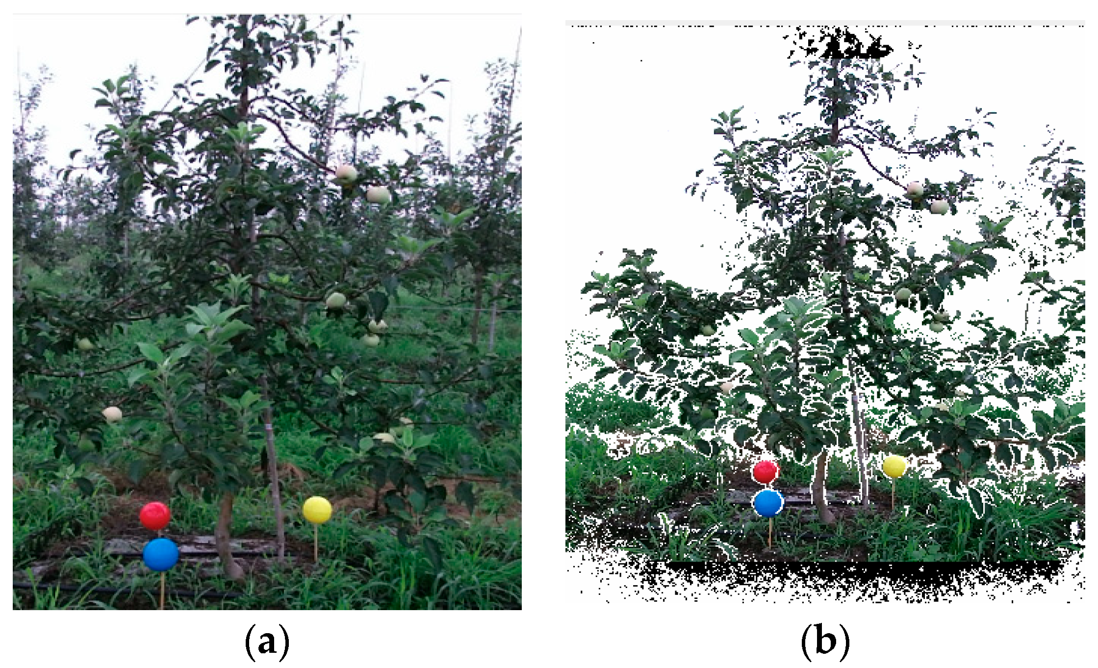
Figure 1 shows a schematic illustration of the measurement system structure. Specifically,
Figure 1a shows a color image of the fruit trees captured by Kinect and
Figure 1b shows the image after depth and color matching for the fruit trees.
The measurement procedure of the fruit tree canopy 3D morphological measurement system based on Kinect sensor self-calibration is shown in
Figure 2. The first step was to initialize the measurement parameters. An appropriate camera shooting position was selected considering the actual scene and terrain conditions. The key factors included the measurement angle, measurement distance and camera height (the measurement angle choice captured the whole fruit tree within the camera’s field of view, the measurement distance was 150–350 cm and the camera was placed at half the height of a given fruit tree). The RYB balls were placed around the trunk and it was verified that the three balls were not obscured at any angle when the fruit tree was shot by the cameras. The second step was to acquire fruit tree RGB-D images under multiple visual angles. According to the requirements and the actual conditions, the required number of visual angles was determined. A nonfixed angle was adopted in the visual angle acquisition (as long as it was verified that the visual angle acquisition can meet the panoramic recovery requirements) and RGB-D images were then acquired by turns under each visual angle. In this paper, we adopted two single visual angle measurement modes (V1 and V2) and a double visual angle measurement mode (with V1 and V2 merged). The third step was to generate the 3D point cloud for a single visual angle. Using the Kinect camera’s internal parameters, the single-visual-angle RGB-D images were converted into a 3D point cloud image. The fruit tree bounding box segmentation and denoising were performed for the 3D point cloud. The fourth step was to reconstruct the fruit tree 3D point cloud. The point cloud coordinates of the three balls under a single visual angle were identified. According to the spherical coordinates of these calibration balls at different angles, the corresponding spatial transition matrix was obtained. The matrix was applied to the fruit tree point cloud under multiple visual angles to achieve the unification of the coordinate system, thereby completing the coarse matching of the fruit tree 3D point cloud. Finally, the iterative closest point (ICP) algorithm was used for self-registration to obtain the complete model of the fruit tree 3D point cloud.
2.2. Procedure of 3D Reconstruction
The first step is to collect the RGB-D image for each visual angle. Considering the fruit tree planting distance in the actual orchard, two visual angles were chosen for the reconstruction. According to the Kinect sensor’s internal parameters, the 3D point cloud image of a single visual angle was converted. The bounding box was used to remove the interfering pixels of the surrounding environment, and outlier denoising was used to cancel out the unrelated noise, thereby generating a preprocessed single-visual-angle 3D point cloud image.
Figure 3 illustrates the 3D reconstruction of two visual angles of the fruit tree; point cloud coordinates are set as PointCloud1 and PointCloud2.
According to the bounding box of each ball and the threshold of color, the point cloud coordinates of the RYB balls were segmented and identified.
Figure 4 shows the specific identification results, the numbers of red ball points were 127 and 161, yellow were 143 and 132, and blue were 193 and 82. The numbers of points can thus satisfy the subsequent processing requirements. The spherical coordinates R1 (
x,
y,
z), Y1 (
x,
y,
z), B1 (
x,
y,
z), R2 (
x,
y,
z), Y2 (
x,
y,
z), and B2 (
x,
y,
z) for the red, yellow, and blue balls under each visual angle were calculated. Next, according to the obtained coordinate values for R1, Y1, B1, and R2, Y2, B2, the formula M (
x,
y,
z) = mean (R, Y, B) was used to calculate the centers of gravity M1 (
x,
y,
z) and M2 (
x,
y,
z) of the triangle determined by the three ball centers in each angle. According to the three points R1, Y1, and B1, plane s1 was determined, and according to R2, Y2, and B2, plane s2 was determined. Thus, point M1 was determined on plane s1, and point M2 was determined on plane s2. Taking points M1 and M2 as the respective vertices for plane s1 and plane s2, their corresponding normal vectors p1 (
a,
b,
c) and p2 (
a,
b,
c) were calculated. Moving points M1 and M2 to the origin O (0, 0, 0) in the coordinate system and translating the vectors p1 and p2 along with M1 and M2 at the same time, the apexes of p1 and p2 would both be at O (0, 0, 0) after the translation; these were then normalized and denoted as p3 and p4. According to the point cloud translation equation PointCloud’ = PointCloud − M, the PointCloud1 and PointCloud2 point cloud coordinates were translated to obtain PointCloud3 and PointCloud4, respectively.
Figure 5 shows the cloud images PointCloud3 and PointCloud4, with point M translated to the origin O (0, 0, 0) for each visual angle point and the normal vectors p3 and p4 that were normal to the plane of the ball centers of the three colored balls.
Rotating the normal vectors p3 and p4 to the Z axis (0, 0, 1) of the Kinect coordinate system and determining the spatial transformation rotation matrices of p3 and p4, Rx1, Ry1 and Rx2, and Ry2, respectively, were calculated. The calculation process was as below: first, the vectors p3 and p4 were rotated α degrees around the X axis to the XOY plane, with the corresponding rotation matrix being Rx (α) (as shown in Equation (1)), and then they were rotated β degrees around the Y axis to the Z axis, with the corresponding rotation matrix being Ry (β) (as shown in Equation (2)), i.e., z (0, 0, 1) = pi × Rx (α)× Ry (β). According to the obtained Rx (α) and Ry (β), the coordinates Y1′ and Y2′ after the translation operation with M for points Y1 and Y2 were connected with the origin O. Likewise, for vectors OY1′ and OY2′, the rotation matrix operations were performed for Rx (α) and Ry (β), and two vectors NOY1 and NOY2 were obtained (with the O as the vertex and with the vectors and as the directions). Finding the size of angle γ between the two vectors NOY1 and NOY2 at this point and substituting γ into Equation (3), the rotation matrix Rz (γ) around the Z axis can be calculated. According to Equation (4), the point clouds upon the spatial transformation for the other visual angles relative to the first visual angle can be obtained.
The point cloud of the first visual angle, along with the point clouds of the other visual angles that were subjected to the above spatial transformation, was displayed in the same point cloud coordinate system, and the 3D point cloud image after coarse registration was obtained (
Figure 6).
where:
PointCloudm is point cloud of the view m; (
x,
y,
z) is point cloud coordinates;
PointCloud’m is point cloud scattered after transformation of the second view space;
Rx (α) is rotation matrix of the normal vector to XOY plane,
Ry (β) is rotation matrix of the normal vector to Z axis; and
Rz (γ) is the rotation matrix around Z axis for angle γ between the two vectors NOY1 and NOY2.
The point cloud image after the coarse registration already had the basic parameters and shape of a fruit tree. However, due to the inherent error in the Kinect acquisition and the calculation error in the calibration process, the coarse registration cannot guarantee accurate information on the point cloud details, and further high-precision fine-tuning registration is needed. According to the ICP algorithm, an iterative registration algorithm proposed by Besl and McKay (1992) [
19], free surfaces and curves can be registered, as well as point clouds. Moreover, the ICP algorithm does not need the accurate information of the initial calibration reference point or the calibration point; it uses iteration to find the nearest point for all the points in the desired registration point cloud, and then continues to calculate the spatial transition matrix by using these known points as standard points until the preset number of times is reached or the set convergence threshold condition is met.
Figure 7 is a model of the fruit tree 3D point cloud after precise registration via ICP, containing accurate 3D information (HWD) about the fruit tree. At this point, the fruit tree 3D reconstruction is completed.
2.3. Calculation Method for the 3D Morphology of the Fruit Tree Canopy
According to the 3D point cloud model of the fruit tree, the fruit tree canopy height (H), the canopy maximum tree width (W) and the canopy thickness (D) were calculated, where D is the length of canopy in the vertical direction. The actual data obtained by measured measurements were compared with the calculated values and an error analysis was conducted. Since the rotation matrix in the 3D reconstruction was processed by normalization, the distance values in the reconstructed point cloud graph coordinate system would correspond to the actual value. The
Z-axis coordinate of the highest point of the canopy was extracted and was compared with the
Z-axis coordinate of the ground to obtain the difference, and the fruit tree height H can thereby be obtained. The specific calculation formula is shown in Equation (5), and the schematic diagram is shown in
Figure 8a.
While the coverage volume of the fruit tree canopy is large, branches overlapped and both located in the main part of the point cloud, W would be different under different visual angles. The study chose the point cloud to make a projection under the XOY visual angle, and by traversing the maximum distance between the two points under the projection, the maximum value would be the maximum W of the fruit tree canopy. The specific calculation formula is shown in Equation (6), and the schematic diagram is shown in
Figure 8b.
To identify the fruit tree canopy, in this study, kernel smoothing was performed for the
Z-axis point cloud quantity distribution of the 3D point cloud after the fruit tree reconstruction, with the calculation formula shown in Equation (7). The distribution chart of the probability density
f is shown in
Figure 9. According to the statistics, setting the threshold as 3 × 10
−4 and setting the probability density greater than the threshold for the first time as the minimum value of the canopy height, the difference between the
Zi coordinate corresponding to the threshold and the fruit tree top
Zmax was calculated. The thickness of the fruit tree canopy can be obtained, with the calculation formula shown as Equation (8).
where:
Z is the vertical axis value of the point cloud of a fruit tree;
x and
y are the corresponding coordinates of the point cloud under the XOY projection;
n is the total number of samples;
h is the band width; and
K is the kernel smoothing function.


