
Different Shades of Kale—Approaches to Analyze Kale Variety Interrelations


Abstract
:1. Introduction
2. Materials and Methods
2.1. Genotyping Kale and Cabbage Samples Using the Brassica 60K Illumina SNP Array
2.1.1. Plant Material
2.1.2. Genotype Data
2.1.3. Processing of Data and Quality Filtering

| Accession | Group (Origin) | Phenotypic Grouping | Additional Information |
|---|---|---|---|
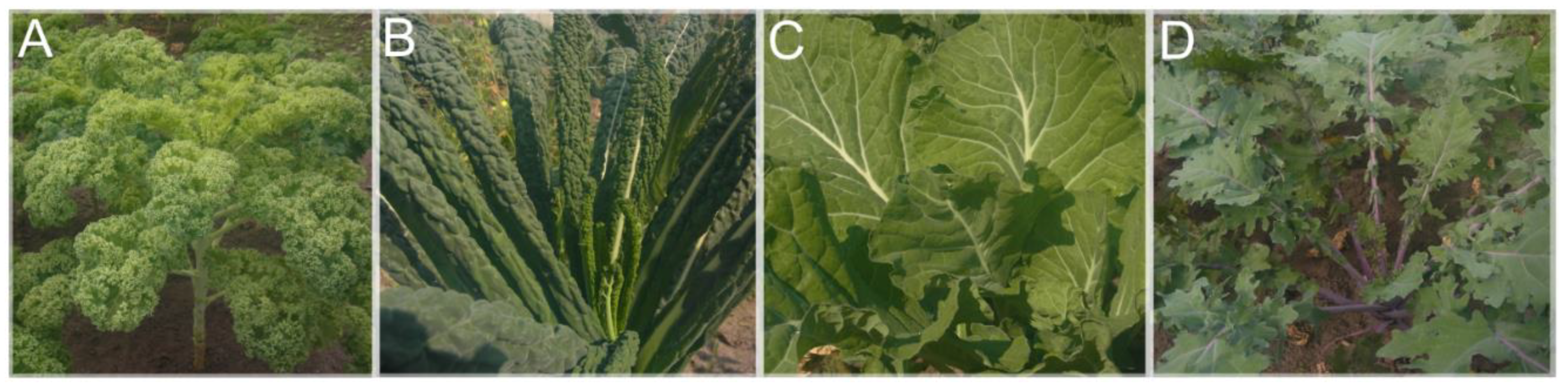
| GER 1–26 | German | curly | |
| OSTFR 1–10 | East Frisian | curly | |
| ITAL 1–13 | Italian | Lacinato-type | |
| ITAL 14–16 | Italian | wild, non-Lacinato | native to Sardinia, Elba island, and Calabria |
| USA 1–7 | American | non-curled collards | USA 5: American farmer-bred curly kale |
| BRASS 1–2 | Russian | lobed/frilled | |
| BRASS 3–5 | wild Brassica | ||
| BOLERA 1–15 | non-kale B. oleracea |
2.2. Employing Linkage Information Using a Published B. napus Genetic Map
2.3. Data Analysis
3. Results
4. Discussion
4.1. Kale Variety Interrelatedness
4.2. SPLoSH Information Improved Analyses of Kale Variety Interrelations
4.3. Curliness as a Criterion for Kale Variety Grouping
4.4. Limitations of Our Analyses
5. Conclusions
Supplementary Materials
Author Contributions
Funding
Institutional Review Board Statement
Informed Consent Statement
Data Availability Statement
Acknowledgments
Conflicts of Interest
References
- Gepts, P. Plant Genetic Resources Conservation and Utilization: The Accomplishments and Future of a Societal Insurance Policy. Crop Sci. 2006, 46, 2278–2292. [Google Scholar] [CrossRef]
- Vellvé, R. The decline of diversity in European agriculture. Ecologist 1993, 23, 64–69. [Google Scholar]
- Mabry, M.E.; Turner-Hissong, S.D.; Gallagher, E.Y.; McAlvay, A.C.; An, H.; Edger, P.P.; Moore, J.D.; Pink, D.A.C.; Teakle, G.R.; Stevens, C.J.; et al. The Evolutionary History of Wild, Domesticated, and Feral Brassica oleracea (Brassicaceae). Mol. Biol. Evol. 2021, 38, 4419–4434. [Google Scholar] [CrossRef] [PubMed]
- Maggioni, L.; von Bothmer, R.; Poulsen, G.; Branca, F. Origin and Domestication of Cole Crops (Brassica oleracea L.): Linguistic and Literary Considerations. Econ. Bot. 2010, 64, 109–123. [Google Scholar] [CrossRef]
- Maggioni, L.; von Bothmer, R.; Poulsen, G.; Lipman, E. Domestication, diversity and use of Brassica oleracea L., based on ancient Greek and Latin texts. Genet. Resour. Crop Evol. 2018, 65, 137–159. [Google Scholar] [CrossRef] [Green Version]
- Hodgkin, T. Cabbages, kales, etc. Brassica oleracea (Cruciferae). In Evolution of Crop Plants, 2nd ed.; Smartt, J.S.N.W., Ed.; Longman Scientific & Technical: Harlow, UK, 1995; pp. 76–82. [Google Scholar]
- Swarup, V.; Brahmi, P. Cole crops. In Plant Genetic Resources: Horticultural Crops; Dhillon, B., Tyagi, R., Saxena, S., Randhawa, G., Eds.; Narosa Publishing House Pvt. Ltd.: New Delhi, India, 2005; pp. 75–88. [Google Scholar]
- Schiemann, E. Entstehung Der Kulturpflanzen; Gebrüder Borntraeger: Berlin, Germany, 1932. [Google Scholar]
- Lizgunova, T. The history of botanical studies of the cabbage, Brassica oleracea L. Bull. Appl. Bot. Genet. Plant Breed. 1959, 32, 37–70. [Google Scholar]
- Mei, J.; Li, Q.; Yang, X.; Qian, L.; Liu, L.; Yin, J.; Frauen, M.; Li, J.; Qian, W. Genomic relationships between wild and cultivated Brassica oleracea L. with emphasis on the origination of cultivated crops. Genet. Resour. Crop Evol. 2010, 57, 687–692. [Google Scholar] [CrossRef]
- Albach, D.; Mageney, V.; Hahn, C. Grünkohl—Ein zu wenig beachtetes Gemüse. Food Lab. 2017, 2, 6–10. [Google Scholar]
- Hahn, C.; Müller, A.; Kuhnert, N.; Albach, D. Diversity of Kale (Brassica oleracea var. sabellica): Glucosinolate Content and Phylogenetic Relationships. J. Agric. Food Chem. 2016, 64, 3215–3225. [Google Scholar] [CrossRef]
- Okumus, A.; Balkaya, A. Estimation of genetic diversity among Turkish kale populations (Brassica oleracea var. acephala L.) using RAPD markers. Russ. J. Genet. 2007, 43, 411–415. [Google Scholar] [CrossRef]
- Christensen, S.; von Bothmer, R.; Poulsen, G.; Maggioni, L.; Phillip, M.; Andersen, B.A.; Jørgensen, R.B. AFLP analysis of genetic diversity in leafy kale (Brassica oleracea L. convar. acephala (DC.) Alef.) landraces, cultivars and wild populations in Europe. Genet. Resour. Crop Evol. 2011, 58, 657–666. [Google Scholar] [CrossRef]
- Branca, F.; Ragusa, L.; Tribulato, A.; Poulsen, G.; Maggioni, L.; von Bothmer, R. Diversity of kale growing in Europe as a basis for crop improvement. In Proceedings of the VI IS on Brassicas and XVIII Crucifer Genetics Workshop; ISHS: Catania, Italy, 2013; pp. 141–147. [Google Scholar] [CrossRef]
- Maggioni, L.; von Bothmer, R.; Poulsen, G.; Branca, F.; Bagger Jørgensen, R. Genetic diversity and population structure of leafy kale and Brassica rupestris Raf. in south Italy. Hereditas 2014, 151, 145–158. [Google Scholar] [CrossRef] [PubMed] [Green Version]
- Farnham, M.W. Genetic Variation among and within United States Collard Cultivars and Landraces as Determined by Randomly Amplified Polymorphic DNA Markers. J. Am. Soc. Hortic. Sci. 1996, 121, 374–379. [Google Scholar] [CrossRef] [Green Version]
- Pelc, S.E.; Couillard, D.M.; Stansell, Z.J.; Farnham, M.W. Genetic Diversity and Population Structure of Collard Landraces and their Relationship to Other Brassica oleracea Crops. Plant Genome 2015, 8, 1–11. [Google Scholar] [CrossRef] [PubMed]
- Arias, T.; Niederhuth, C.E.; McSteen, P.; Pires, J.C. The Molecular Basis of Kale Domestication: Transcriptional Profiling of Developing Leaves Provides New Insights Into the Evolution of a Brassica oleracea Vegetative Morphotype. Front. Plant Sci. 2021, 12, 637115:1–637115:17. [Google Scholar] [CrossRef] [PubMed]
- Megías-Pérez, R.; Hahn, C.; Ruiz-Matute, A.I.; Behrends, B.; Albach, D.C.; Kuhnert, N. Changes in low molecular weight carbohydrates in kale during development and acclimation to cold temperatures determined by chromatographic techniques coupled to mass spectrometry. Food Res. Int. 2020, 127, 108727:1–108727:9. [Google Scholar] [CrossRef] [PubMed]
- Tonguç, M.; Griffiths, P.D. Genetic relationships of Brassica vegetables determined using database derived simple sequence repeats. Euphytica 2004, 137, 193–201. [Google Scholar] [CrossRef]
- Warwick, S.I.; Sauder, C.A. Phylogeny of tribe Brassiceae (Brassicaceae) based on chloroplast restriction site polymorphisms and nuclear ribosomal internal transcribed spacer and chloroplast trnL intron sequences. Can. J. Bot. 2005, 83, 467–483. [Google Scholar] [CrossRef]
- Flannery, M.L.; Mitchell, F.J.; Coyne, S.; Kavanagh, T.A.; Burke, J.I.; Salamin, N.; Dowding, P.; Hodkinson, T.R. Plastid genome characterisation in Brassica and Brassicaceae using a new set of nine SSRs. Theor. Appl. Genet. 2006, 113, 1221–1231. [Google Scholar] [CrossRef]
- Louarn, S.; Torp, A.M.; Holme, I.B.; Andersen, S.B.; Jensen, B.D. Database derived microsatellite markers (SSRs) for cultivar differentiation in Brassica oleracea. Genet. Resour. Crop Evol. 2007, 54, 1717–1725. [Google Scholar] [CrossRef]
- Lü, N.; Yamane, K.; Ohnishi, O. Genetic diversity of cultivated and wild radish and phylogenetic relationships among Raphanus and Brassica species revealed by the analysis of trnK/matK sequence. Breed. Sci. 2008, 58, 15–22. [Google Scholar] [CrossRef] [Green Version]
- Izzah, N.K.; Lee, J.; Perumal, S.; Park, J.Y.; Ahn, K.; Fu, D.; Kim, G.-B.; Nam, Y.-W.; Yang, T.-J. Microsatellite-based analysis of genetic diversity in 91 commercial Brassica oleracea L. cultivars belonging to six varietal groups. Genet. Resour. Crop Evol. 2013, 60, 1967–1986. [Google Scholar] [CrossRef]
- Semagn, K.; Babu, R.; Hearne, S.; Olsen, M. Single nucleotide polymorphism genotyping using Kompetitive Allele Specific PCR (KASP): Overview of the technology and its application in crop improvement. Mol. Breed. 2014, 33, 1–14. [Google Scholar] [CrossRef]
- Schlötterer, C. The evolution of molecular markers—Just a matter of fashion? Nat. Rev. Genet. 2004, 5, 63–69. [Google Scholar] [CrossRef] [PubMed]
- Liu, N.; Chen, L.; Wang, S.; Oh, C.; Zhao, H. Comparison of single-nucleotide polymorphisms and microsatellites in inference of population structure. BMC Genet. 2005, 6 (Suppl. 1), S26:1–S26:5. [Google Scholar] [CrossRef] [PubMed] [Green Version]
- Haasl, R.J.; Payseur, B.A. Multi-locus inference of population structure: A comparison between single nucleotide polymorphisms and microsatellites. Heredity 2011, 106, 158–171. [Google Scholar] [CrossRef] [PubMed] [Green Version]
- Dalton-Morgan, J.; Hayward, A.; Alamery, S.; Tollenaere, R.; Mason, A.S.; Campbell, E.; Patel, D.; Lorenc, M.T.; Yi, B.; Long, Y.; et al. A high-throughput SNP array in the amphidiploid species Brassica napus shows diversity in resistance genes. Funct. Integr. Genom. 2014, 14, 643–655. [Google Scholar] [CrossRef] [PubMed]
- Paritosh, K.; Gupta, V.; Yadava, S.K.; Singh, P.; Pradhan, A.K.; Pental, D. RNA-seq based SNPs for mapping in Brassica juncea (AABB): Synteny analysis between the two constituent genomes A (from B. rapa) and B (from B. nigra) shows highly divergent gene block arrangement and unique block fragmentation patterns. BMC Genom. 2014, 15, 396:1–396:14. [Google Scholar] [CrossRef] [Green Version]
- Cheng, F.; Sun, R.; Hou, X.; Zheng, H.; Zhang, F.; Zhang, Y.; Liu, B.; Liang, J.; Zhuang, M.; Liu, Y.; et al. Subgenome parallel selection is associated with morphotype diversification and convergent crop domestication in Brassica rapa and Brassica oleracea. Nat. Genet. 2016, 48, 1218–1224. [Google Scholar] [CrossRef]
- Bird, K.A.; An, H.; Gazave, E.; Gore, M.A.; Pires, J.C.; Robertson, L.D.; Labate, J.A. Population Structure and Phylogenetic Relationships in a Diverse Panel of Brassica rapa L. Front. Plant Sci. 2017, 8, 321:1–321:12. [Google Scholar] [CrossRef] [Green Version]
- Stansell, Z.; Hyma, K.; Fresnedo-Ramírez, J.; Sun, Q.; Mitchell, S.; Björkman, T.; Hua, J. Genotyping-by-sequencing of Brassica oleracea vegetables reveals unique phylogenetic patterns, population structure and domestication footprints. Hortic. Res. 2018, 5, 38:1–38:10. [Google Scholar] [CrossRef] [PubMed] [Green Version]
- Robinson, P.; Holme, J. KASP Version 4.0 SNP Genotyping Manual. Available online: https://www.cerealsdb.uk.net/cerealgenomics/CerealsDB/PDFs/KASP_SNP_Genotyping_Manual.pdf (accessed on 20 December 2021).
- Arias, T.; Pires, J.C. A fully resolved chloroplast phylogeny of the brassica crops and wild relatives (Brassicaceae: Brassiceae): Novel clades and potential taxonomic implications. Taxon 2012, 61, 980–988. [Google Scholar] [CrossRef]
- Kumpatla, S.P.; Buyyarapu, R.; Abdurakhmonov, I.Y.; Mammadov, J.A. Genomics-assisted plant breeding in the 21st century: Technological advances and progress. In Plant Breeding; Abdurakhmonov, I., Ed.; InTech: Rijeka, Croatia, 2012; pp. 131–184. [Google Scholar]
- Clarke, W.E.; Higgins, E.E.; Plieske, J.; Wieseke, R.; Sidebottom, C.; Khedikar, Y.; Batley, J.; Edwards, D.; Meng, J.; Li, R.; et al. A high-density SNP genotyping array for Brassica napus and its ancestral diploid species based on optimised selection of single-locus markers in the allotetraploid genome. Theor. Appl. Genet. 2016, 129, 1887–1899. [Google Scholar] [CrossRef] [PubMed] [Green Version]
- Nagaharu, U. Genome analysis in Brassica with special reference to the experimental formation of B. napus and peculiar mode of fertilization. Jpn. J. Bot. 1935, 7, 389–452. [Google Scholar]
- Rousseau-Gueutin, M.; Morice, J.; Coriton, O.; Huteau, V.; Trotoux, G.; Negre, S.; Falentin, C.; Deniot, G.; Gilet, M.; Eber, F.; et al. The Impact of Open Pollination on the Structural Evolutionary Dynamics, Meiotic Behavior, and Fertility of Resynthesized Allotetraploid Brassica napus L. G3 2017, 7, 705–717. [Google Scholar] [CrossRef] [PubMed] [Green Version]
- Stein, A.; Coriton, O.; Rousseau-Gueutin, M.; Samans, B.; Schiessl, S.V.; Obermeier, C.; Parkin, I.A.P.; Chevre, A.M.; Snowdon, R.J. Mapping of homoeologous chromosome exchanges influencing quantitative trait variation in Brassica napus. Plant Biotechnol. J. 2017, 15, 1478–1489. [Google Scholar] [CrossRef] [PubMed] [Green Version]
- Wei, D.; Cui, Y.; He, Y.; Xiong, Q.; Qian, L.; Tong, C.; Lu, G.; Ding, Y.; Li, J.; Jung, C.; et al. A genome-wide survey with different rapeseed ecotypes uncovers footprints of domestication and breeding. J. Exp. Bot. 2017, 68, 4791–4801. [Google Scholar] [CrossRef] [Green Version]
- Yang, Y.; Shen, Y.; Li, S.; Ge, X.; Li, Z. High Density Linkage Map Construction and QTL Detection for Three Silique-Related Traits in Orychophragmus violaceus Derived Brassica napus Population. Front. Plant Sci. 2017, 8, 1512:1–1512:13. [Google Scholar] [CrossRef] [Green Version]
- Higgins, E.E.; Clarke, W.E.; Howell, E.C.; Armstrong, S.J.; Parkin, I.A.P. Detecting de Novo Homoeologous Recombination Events in Cultivated Brassica napus Using a Genome-Wide SNP Array. G3 2018, 8, 2673–2683. [Google Scholar] [CrossRef] [Green Version]
- Valdés, A.; Clemens, R.; Möllers, C. Mapping of quantitative trait loci for microspore embryogenesis-related traits in the oilseed rape doubled haploid population DH4069 × Express 617. Mol. Breed. 2018, 38, 65:1–65:15. [Google Scholar] [CrossRef]
- Luo, X.; Tan, Y.; Ma, C.; Tu, J.; Shen, J.; Yi, B.; Fu, T. High-throughput identification of SNPs reveals extensive heterosis with intra-group hybridization and genetic characteristics in a large rapeseed (Brassica napus L.) panel. Euphytica 2019, 215, 157:1–157:10. [Google Scholar] [CrossRef]
- Wu, J.; Chen, P.; Zhao, Q.; Cai, G.; Hu, Y.; Xiang, Y.; Yang, Q.; Wang, Y.; Zhou, Y. Co-location of QTL for Sclerotinia stem rot resistance and flowering time in Brassica napus. Crop J. 2019, 7, 227–237. [Google Scholar] [CrossRef]
- Zhang, F.; Huang, J.; Tang, M.; Cheng, X.; Liu, Y.; Tong, C.; Yu, J.; Sadia, T.; Dong, C.; Liu, L.; et al. Syntenic quantitative trait loci and genomic divergence for Sclerotinia resistance and flowering time in Brassica napus. J. Integr. Plant Biol. 2019, 61, 75–88. [Google Scholar] [CrossRef] [PubMed] [Green Version]
- Li, B.; Gao, J.; Chen, J.; Wang, Z.; Shen, W.; Yi, B.; Wen, J.; Ma, C.; Shen, J.; Fu, T.; et al. Identification and fine mapping of a major locus controlling branching in Brassica napus. Theor. Appl. Genet. 2020, 133, 771–783. [Google Scholar] [CrossRef]
- Helal, M.; Gill, R.A.; Tang, M.; Yang, L.; Hu, M.; Yang, L.; Xie, M.; Zhao, C.; Cheng, X.; Zhang, Y.; et al. SNP- and Haplotype-Based GWAS of Flowering-Related Traits in Brassica napus. Plants 2021, 10, 2475. [Google Scholar] [CrossRef]
- Raman, H.; Raman, R.; Qiu, Y.; Zhang, Y.; Batley, J.; Liu, S. The Rlm13 Gene, a New Player of Brassica napus-Leptosphaeria maculans Interaction Maps on Chromosome C03 in Canola. Front. Plant Sci. 2021, 12, 654604:1–654604:14. [Google Scholar] [CrossRef]
- Zeng, C.L.; Wan, H.P.; Wu, X.M.; Dai, X.G.; Chen, J.D.; Ji, Q.Q.; Qian, F. Genome-wide association study of low nitrogen tolerance traits at the seedling stage of rapeseed. Biol. Plant. 2021, 65, 10–18. [Google Scholar] [CrossRef]
- Brown, A.F.; Yousef, G.G.; Chebrolu, K.K.; Byrd, R.W.; Everhart, K.W.; Thomas, A.; Reid, R.W.; Parkin, I.A.; Sharpe, A.G.; Oliver, R.; et al. High-density single nucleotide polymorphism (SNP) array mapping in Brassica oleracea: Identification of QTL associated with carotenoid variation in broccoli florets. Theor. Appl. Genet. 2014, 127, 2051–2064. [Google Scholar] [CrossRef]
- Mei, J.; Wang, J.; Li, Y.; Tian, S.; Wei, D.; Shao, C.; Si, J.; Xiong, Q.; Li, J.; Qian, W. Mapping of genetic locus for leaf trichome in Brassica oleracea. Theor. Appl. Genet. 2017, 130, 1953–1959. [Google Scholar] [CrossRef]
- Peng, L.; Zhou, L.; Li, Q.; Wei, D.; Ren, X.; Song, H.; Mei, J.; Si, J.; Qian, W. Identification of Quantitative Trait Loci for Clubroot Resistance in Brassica oleracea With the Use of Brassica SNP Microarray. Front. Plant Sci. 2018, 9, 822:1–822:8. [Google Scholar] [CrossRef]
- Ganal, M.W.; Polley, A.; Graner, E.M.; Plieske, J.; Wieseke, R.; Luerssen, H.; Durstewitz, G. Large SNP arrays for genotyping in crop plants. J. Biosci. 2012, 37, 821–828. [Google Scholar] [CrossRef] [PubMed]
- Howard, N.P.; Peace, C.; Silverstein, K.A.T.; Poets, A.; Luby, J.J.; Vanderzande, S.; Durel, C.E.; Muranty, H.; Denance, C.; van de Weg, E. The use of shared haplotype length information for pedigree reconstruction in asexually propagated outbreeding crops, demonstrated for apple and sweet cherry. Hortic. Res. 2021, 8, 202:1–202:13. [Google Scholar] [CrossRef] [PubMed]
- Lee, J.; Izzah, N.K.; Choi, B.S.; Joh, H.J.; Lee, S.C.; Perumal, S.; Seo, J.; Ahn, K.; Jo, E.J.; Choi, G.J.; et al. Genotyping-by-sequencing map permits identification of clubroot resistance QTLs and revision of the reference genome assembly in cabbage (Brassica oleracea L.). DNA Res. 2016, 23, 29–41. [Google Scholar] [CrossRef] [PubMed] [Green Version]
- Branham, S.E.; Stansell, Z.J.; Couillard, D.M.; Farnham, M.W. Quantitative trait loci mapping of heat tolerance in broccoli (Brassica oleracea var. italica) using genotyping-by-sequencing. Theor. Appl. Genet. 2017, 130, 529–538. [Google Scholar] [CrossRef] [PubMed]
- Zhao, Z.; Gu, H.; Sheng, X.; Yu, H.; Wang, J.; Huang, L.; Wang, D. Genome-Wide Single-Nucleotide Polymorphisms Discovery and High-Density Genetic Map Construction in Cauliflower Using Specific-Locus Amplified Fragment Sequencing. Front. Plant Sci. 2016, 7, 334:1–334:9. [Google Scholar] [CrossRef] [PubMed] [Green Version]
- Stansell, Z.; Farnham, M.; Bjorkman, T. Complex Horticultural Quality Traits in Broccoli Are Illuminated by Evaluation of the Immortal BolTBDH Mapping Population. Front. Plant Sci. 2019, 10, 1104:1–1104:20. [Google Scholar] [CrossRef]
- Illumina®. Infinium® HD Assay: Ultra Protocol Guide. Available online: https://support.illumina.com/content/dam/illumina-support/documents/documentation/chemistry_documentation/infinium_assays/infinium-hd-ultra/11328087_RevB_Infinium_HD_Ultra_Assay_Guide_press.pdf (accessed on 20 December 2021).
- Gunderson, K.L.; Kuhn, K.M.; Steemers, F.J.; Ng, P.; Murray, S.S.; Shen, R. Whole-genome genotyping of haplotype tag single nucleotide polymorphisms. Pharmacogenomics 2006, 7, 641–648. [Google Scholar] [CrossRef] [Green Version]
- Gladis, T.; Hammer, K. Nomenclatural notes on the Brassica oleracea-group. Genet. Resour. Crop Evol. 2001, 48, 7–11. [Google Scholar] [CrossRef]
- R Core Team. R: A Language and Environment for Statistical Computing; R Foundation for Statistical Computing: Vienna, Austria, 2021. [Google Scholar]
- Josse, J.; Husson, F. missMDA: A Package for Handling Missing Values in Multivariate Data Analysis. J. Stat. Softw. 2016, 70, 1–31. [Google Scholar] [CrossRef]
- Wickham, H. ggplot2: Elegant Graphics for Data Analysis, 1st ed.; Springer: New York, NY, USA, 2016; p. 213. [Google Scholar]
- Jombart, T. Adegenet: A R package for the multivariate analysis of genetic markers. Bioinformatics 2008, 24, 1403–1405. [Google Scholar] [CrossRef] [Green Version]
- Pritchard, J.K.; Stephens, M.; Donnelly, P. Inference of population structure using multilocus genotype data. Genetics 2000, 155, 945–959. [Google Scholar] [CrossRef] [PubMed]
- Falush, D.; Stephens, M.; Pritchard, J.K. Inference of population structure using multilocus genotype data: Linked loci and correlated allele frequencies. Genetics 2003, 164, 1567–1587. [Google Scholar] [CrossRef] [PubMed]
- Hubisz, M.J.; Falush, D.; Stephens, M.; Pritchard, J.K. Inferring weak population structure with the assistance of sample group information. Mol. Ecol. Resour. 2009, 9, 1322–1332. [Google Scholar] [CrossRef] [PubMed] [Green Version]
- Evanno, G.; Regnaut, S.; Goudet, J. Detecting the number of clusters of individuals using the software STRUCTURE: A simulation study. Mol. Ecol. 2005, 14, 2611–2620. [Google Scholar] [CrossRef] [Green Version]
- Kopelman, N.M.; Mayzel, J.; Jakobsson, M.; Rosenberg, N.A.; Mayrose, I. CLUMPAK: A program for identifying clustering modes and packaging population structure inferences across K. Mol. Ecol. Resour. 2015, 15, 1179–1191. [Google Scholar] [CrossRef] [Green Version]
- Jakobsson, M.; Rosenberg, N.A. CLUMPP: A cluster matching and permutation program for dealing with label switching and multimodality in analysis of population structure. Bioinformatics 2007, 23, 1801–1806. [Google Scholar] [CrossRef] [Green Version]
- Rosenberg, N.A. DISTRUCT: A program for the graphical display of population structure. Mol. Ecol. Notes 2004, 4, 137–138. [Google Scholar] [CrossRef]
- Bryant, D.; Moulton, V. Neighbor-Net: An agglomerative method for the construction of phylogenetic networks. Mol. Biol. Evol. 2004, 21, 255–265. [Google Scholar] [CrossRef]
- Huson, D.H.; Bryant, D. Application of phylogenetic networks in evolutionary studies. Mol. Biol. Evol. 2006, 23, 254–267. [Google Scholar] [CrossRef]
- Dress, A.W.; Huson, D.H. Constructing splits graphs. IEEE ACM Trans. Comput. Biol. Bioinform. 2004, 1, 109–115. [Google Scholar] [CrossRef]
- Gambette, P.; Huson, D.H. Improved layout of phylogenetic networks. IEEE ACM Trans. Comput. Biol. Bioinform. 2008, 5, 472–479. [Google Scholar] [CrossRef] [PubMed] [Green Version]
- Ronquist, F.; Huelsenbeck, J.P. MrBayes 3: Bayesian phylogenetic inference under mixed models. Bioinformatics 2003, 19, 1572–1574. [Google Scholar] [CrossRef] [PubMed] [Green Version]
- Farnham, M.W.; Davis, E.H.; Morgan, J.T.; Smith, J.P. Neglected landraces of collard (Brassica oleracea L. var. viridis) from the Carolinas (USA). Genet. Resour. Crop Evol. 2008, 55, 797–801. [Google Scholar] [CrossRef]
- Penny, D.; White, W.T.; Hendy, M.D.; Phillips, M.J. A bias in ML estimates of branch lengths in the presence of multiple signals. Mol. Biol. Evol. 2008, 25, 239–242. [Google Scholar] [CrossRef] [PubMed] [Green Version]
- Kennedy, M.; Holland, B.R.; Gray, R.D.; Spencer, H.G. Untangling long branches: Identifying conflicting phylogenetic signals using spectral analysis, neighbor-net, and consensus networks. Syst. Biol. 2005, 54, 620–633. [Google Scholar] [CrossRef] [Green Version]
- Mardulyn, P. Trees and/or networks to display intraspecific DNA sequence variation? Mol. Ecol. 2012, 21, 3385–3390. [Google Scholar] [CrossRef]
- Saitou, N.; Nei, M. The neighbor-joining method: A new method for reconstructing phylogenetic trees. Mol. Biol. Evol. 1987, 4, 406–425. [Google Scholar] [CrossRef]
- Toomajian, C.; Hu, T.T.; Aranzana, M.J.; Lister, C.; Tang, C.; Zheng, H.; Zhao, K.; Calabrese, P.; Dean, C.; Nordborg, M. A nonparametric test reveals selection for rapid flowering in the Arabidopsis genome. PLoS Biol. 2006, 4, e137. [Google Scholar] [CrossRef] [Green Version]
- Cavanagh, C.R.; Chao, S.; Wang, S.; Huang, B.E.; Stephen, S.; Kiani, S.; Forrest, K.; Saintenac, C.; Brown-Guedira, G.L.; Akhunova, A.; et al. Genome-wide comparative diversity uncovers multiple targets of selection for improvement in hexaploid wheat landraces and cultivars. Proc. Natl. Acad. Sci. USA 2013, 110, 8057–8062. [Google Scholar] [CrossRef] [Green Version]
- Jordan, K.W.; Wang, S.; Lun, Y.; Gardiner, L.J.; MacLachlan, R.; Hucl, P.; Wiebe, K.; Wong, D.; Forrest, K.L.; IWGS-Consortium; et al. A haplotype map of allohexaploid wheat reveals distinct patterns of selection on homoeologous genomes. Genome Biol. 2015, 16, 48:1–48:18. [Google Scholar] [CrossRef] [Green Version]
- Poets, A.M.; Mohammadi, M.; Seth, K.; Wang, H.; Kono, T.J.; Fang, Z.; Muehlbauer, G.J.; Smith, K.P.; Morrell, P.L. The Effects of Both Recent and Long-Term Selection and Genetic Drift Are Readily Evident in North American Barley Breeding Populations. G3 2016, 6, 609–622. [Google Scholar] [CrossRef] [PubMed] [Green Version]
- Hao, C.; Wang, Y.; Chao, S.; Li, T.; Liu, H.; Wang, L.; Zhang, X. The iSelect 9 K SNP analysis revealed polyploidization induced revolutionary changes and intense human selection causing strong haplotype blocks in wheat. Sci. Rep. 2017, 7, 41247:1–41247:13. [Google Scholar] [CrossRef] [PubMed]
- Coffman, S.M.; Hufford, M.B.; Andorf, C.M.; Lubberstedt, T. Haplotype structure in commercial maize breeding programs in relation to key founder lines. Theor. Appl. Genet. 2020, 133, 547–561. [Google Scholar] [CrossRef] [PubMed] [Green Version]
- Brinton, J.; Ramirez-Gonzalez, R.H.; Simmonds, J.; Wingen, L.; Orford, S.; Griffiths, S.; Wheat Genome, P.; Haberer, G.; Spannagl, M.; Walkowiak, S.; et al. A haplotype-led approach to increase the precision of wheat breeding. Commun. Biol. 2020, 3, 712:1–712:11. [Google Scholar] [CrossRef]
- Roman, M.G.; Houston, R. Investigation of chloroplast regions rps16 and clpP for determination of Cannabis sativa crop type and biogeographical origin. Leg. Med. 2020, 47, 101759:1–101759:7. [Google Scholar] [CrossRef]
- Wang, Z.; Hao, C.; Zhao, J.; Li, C.; Jiao, C.; Xi, W.; Hou, J.; Li, T.; Liu, H.; Zhang, X. Genomic footprints of wheat evolution in China reflected by a Wheat660K SNP array. Crop J. 2021, 9, 29–41. [Google Scholar] [CrossRef]
- Mason, A.S.; Higgins, E.E.; Snowdon, R.J.; Batley, J.; Stein, A.; Werner, C.; Parkin, I.A. A user guide to the Brassica 60K Illumina Infinium™ SNP genotyping array. Theor. Appl. Genet. 2017, 130, 621–633. [Google Scholar] [CrossRef]


Publisher’s Note: MDPI stays neutral with regard to jurisdictional claims in published maps and institutional affiliations. |
© 2022 by the authors. Licensee MDPI, Basel, Switzerland. This article is an open access article distributed under the terms and conditions of the Creative Commons Attribution (CC BY) license (https://creativecommons.org/licenses/by/4.0/).
Share and Cite
Hahn, C.; Howard, N.P.; Albach, D.C. Different Shades of Kale—Approaches to Analyze Kale Variety Interrelations. Genes 2022, 13, 232. https://doi.org/10.3390/genes13020232
Hahn C, Howard NP, Albach DC. Different Shades of Kale—Approaches to Analyze Kale Variety Interrelations. Genes. 2022; 13(2):232. https://doi.org/10.3390/genes13020232
Chicago/Turabian StyleHahn, Christoph, Nicholas P. Howard, and Dirk C. Albach. 2022. "Different Shades of Kale—Approaches to Analyze Kale Variety Interrelations" Genes 13, no. 2: 232. https://doi.org/10.3390/genes13020232
APA StyleHahn, C., Howard, N. P., & Albach, D. C. (2022). Different Shades of Kale—Approaches to Analyze Kale Variety Interrelations. Genes, 13(2), 232. https://doi.org/10.3390/genes13020232